Parsimonious Random Vector Functional Link Network
for Data Streams
Mahardhika Pratamaa, Plamen P. Angelovb, Edwin Lughoferc, Deepak
Puthald
aSchool of Computer Science and Engineering, Nanyang Technological University, Singapore, 639798,Singapore
bSchool of Computing and Communication, Lancaster University, Lancaster, UK cDepartment of Knowledge-based Mathematical Systems, Johannes Kepler University,
Linz, Austria
dSchool of Electrical and Data Engineering, University of Technology, Sydney, Australia
Abstract
The majority of the existing work on random vector functional link net-works (RVFLNs) is not scalable for data stream analytics because they work under a batched learning scenario and lack a self-organizing property. A novel RVLFN, namely the parsimonious random vector functional link net-work (pRVFLN), is proposed in this paper. pRVFLN adopts a fully flexible and adaptive working principle where its network structure can be config-ured from scratch and can be automatically generated, pruned and recalled from data streams. pRVFLN is capable of selecting and deselecting input attributes on the fly as well as capable of extracting important training sam-ples for model updates. In addition, pRVFLN introduces a non-parametric type of hidden node which completely reflects the real data distribution and is not constrained by a specific shape of the cluster. All learning proce-dures of pRVFLN follow a strictly single-pass learning mode, which is ap-plicable for online time-critical applications. The advantage of pRVFLN is verified through numerous simulations with real-world data streams. It was benchmarked against recently published algorithms where it demonstrated comparable and even higher predictive accuracies while imposing the lowest complexities.
Email addresses: [email protected](Mahardhika Pratama),
[email protected](Plamen P. Angelov),[email protected](Edwin
Keywords: Random Vector Functional Link, Evolving Intelligent System, Online Learning, Online Identification, Randomized Neural Networks
1. Introduction 1
For decades, research in artificial neural networks has mainly investigated
2
the best way to determine network-free parameters, which produces a model
3
with low generalization error. Various approaches were proposed, but a large
4
volume of work is based on a first or second-order derivative approach in
5
respect to the loss function. Due to the rapid technological progress in data
6
storage, capture, and transmission, the machine learning community has
en-7
countered an information explosion, which calls for scalable data analytics.
8
Significant growth of the problem space has led to a scalability issue for
con-9
ventional machine learning approaches, which require iterating entire batches
10
of data over multiple epochs. This phenomenon results in a strong demand
11
for a simple, fast machine learning algorithm to be well-suited for
deploy-12
ment in numerous data-rich applications [1]. This provides a strong case for
13
research in the area of randomness in neural networks [2, 3], which was very
14
popular in the late 80s and early 90s. This concept offers an algorithmic
15
framework, which allows them to generate most of the network parameters
16
randomly while still retaining reasonable performance [3]. One of the most
17
prominent examples of randomness in neural networks is the random vector
18
functional link network (RVFLN) which features solid universal
approxima-19
tion theory under strict conditions [4].
20
Due to its simple but sound working principle, randomness in neural
net-21
works has regained its popularity in the current literature [5, 6, 7, 8, 9].
22
Nonetheless, the vast majority of work in the literature suffers from the
23
issue of complexity which makes their computational complexity and
mem-24
ory burden prohibitive for data stream analytics since their complexities are
25
manually determined and rely heavily on expert domain knowledge. These
26
works present a model with a fixed size which lacks of adaptive mechanism
27
to encounter changing training patterns in the data streams. The random
28
selection of network parameters often causes the network complexity to go
29
beyond what is necessary due to the existence of superfluous hidden nodes
30
which contribute little to the generalization performance [25]. Although the
31
universal approximation capability of such an approach is assured only when
32
sufficient complexity is selected, choosing a suitable complexity for a given
33
problem entails expert-domain knowledge and is problem-dependent.
A novel RVFLN, namely the parsimonious random vector functional link
35
network (pRVFLN), is proposed. pRVFLN combines the simple and fast
36
working principles of RFVLN where all network parameters but the output
37
weights are randomly generated with no tuning mechanism for hidden nodes.
38
It characterises the online and adaptive nature of evolving intelligent systems.
39
pRVFLN is capable of tracking any variations of data streams no matter how
40
slow, rapid, gradual, sudden or temporal the drifts in data streams because it
41
can initiate its learning structure from scratch with no initial structure and its
42
structure is self-evolved from data streams in the one-pass learning mode by
43
automatically adding, pruning and recalling its hidden nodes [10].
Further-44
more, it is compatible for online real-time deployment because data streams
45
are handled without revisiting previously seen samples. pRVFLN is equipped
46
with a hidden node pruning mechanism which guarantees a low structural
47
burden and the rule recall mechanism which aims to address cyclic concept
48
drift. pRVFLN incorporates a dynamic input selection scenario which makes
49
possible the activation and deactivation of input attributes on the fly and
50
an online active learning scenario which rules out inconsequential samples
51
from the training process. pRVFLN is a plug-and-play learner where a single
52
training process encompasses all learning scenarios in a sample-wise
man-53
ner without pre-and/or post-processing steps. pRVFLN offers at least four
54
novelties: 1) it introduces the interval-valued data cloud paradigm which is
55
an extension of the data cloud in [11]. This modification aims to induce
56
robustness in dealing with data uncertainty caused by noisy measurement,
57
noisy data, etc. Unlike conventional hidden nodes, the interval-valued data
58
cloud is parameter-free and requires no parametrization. It evolves naturally,
59
similar to real data distribution; 2) an online active learning scenario based
60
on the sequential entropy method (SEM) is proposed. The SEM is derived
61
from the concept of neighbourhood probability [12] but here the concept of
62
the data cloud is integrated. The data cloud concept simplifies the sample
63
selection process because the neighbourhood probability is inferred with ease
64
from the activation degree of the data cloud; 3) pRVFLN is capable of
au-65
tomatically generating its hidden nodes on the fly with the help of a type-2
66
self-constructing clustering (T2SCC) mechanism [13, 14]. This rule growing
67
process differs from existing approaches because the hidden nodes are
cre-68
ated from the rule growing condition, which considers the locations of the
69
data samples in the input space; 4) pRVFLN is capable of carrying out an
70
online feature selection process, borrowing several concepts of online feature
71
selection (OFS) [15]. The original version [15] is generalized here since it
is originally devised for linear regression and calls for some modification to
73
be a perfect fit for pRVLFN. The prominent trait of this method lies in a
74
flexible online feature selection scenario, which makes it possible to select or
75
deselect input attributes on demand by assigning crisp weights (0 or 1) to
76
input features.
77
The efficacy of pRVFLN was thoroughly evaluated using numerous
real-78
world data streams and was benchmarked against recently published
algo-79
rithms in the literature, with pRVFLN demonstrating a highly scalable
ap-80
proach for data stream analytics while retaining acceptable generalization
81
performance. An analysis of the robustness of random intervals was
per-82
formed. It is concluded that random regions should be carefully selected
83
and should be chosen close to the true operating regions of a system being
84
modelled. Moreover, we also present a sensitivity analysis of the predefined
85
threshold and study the effect of learning components. A supplemental
doc-86
ument containing additional numerical studies is also provided in 1 and the
87
MATLAB codes of pRVFLN have been made publicly available in 2 to help
88
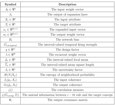
further study. Key mathematical notations are listed in Table 1.
89
The rest of this paper is structured as follows: the network architecture of
90
pRVFLN is outlined in Section 2; the algorithmic development of pRVFLN is
91
detailed in Section 3; proof of concept is outlined in Section 4; and conclusions
92
are drawn in the last section of this paper.
93
2. Related Work 94
The concept of randomness in neural networks was initiated by
Broom-95
head and Iowe in their work on radial basis function networks (RBFNs)
96
[3]. A closed pseudo-inverse solution can be formulated to obtain the output
97
weights of the RBFN and the centres of RBF units can be randomly sampled
98
from data samples. This work later was generalized in [16], where the centre
99
of the RBF neurons can be sampled from an independent distribution of the
100
training data. The randomness in neural networks was substantiated by the
101
findings of White [9], who developed a statistical test on hidden nodes. It
102
was found that some nonlinear structures in the mapping function can be
103
neglected without substantial loss of accuracy. In [9], the input weights of
104
1https://www.dropbox.com/s/lytpt4huqyoqa6p/supplemental document.docx?dl=0
the hidden layers are randomly chosen. It is shown that the input weights
105
are not sensitive to the overall learning performance.
106
A prominent contribution was made by Pao et al. with the random vector
107
functional link network (RVFLN) [17]. This work presents a specific case of
108
the functional link neural network [18], which embraces the concept of
ran-109
domness in the functional link network. Note that a closed pseudo-inversion
110
solution can be also defined for the RVFLN in lieu of the conjugate gradient
111
(CG) approach. The universal approximation capability of the RVFLN is
112
proven in [4] by formalising the Monte Carlo method approximating a
limit-113
integral representation of a function. To attain the universal approximation
114
capability, the hidden node should be chosen as either absolutely integrable or
115
differentiable function. In practise, the region of random parameters should
116
also be chosen carefully and the number of hidden nodes should be sufficiently
117
large. There also exists another research direction in this area, namely
reser-118
voir computing (RC), which puts forward a recurrent network architecture in
119
order to take into account temporal dependencies between subsequent
pat-120
terns and in order to avoid dependencies on time-delayed input attributes
121
[19]. RC is constructed with a fixed number of recurrent layers and adopts
122
the concept of randomness in neural network where all the parameters are
123
randomly generated except the output weight. A comprehensive survey of
124
randomness in neural network can be found in [2, 6].
125
Since the last decade, RVFLN has transformed into one of the most
vi-126
brant fields in the neural network community as evidenced by its numerous
127
extensions and variations. The vast majority of RNNs in the literature are
128
not compatible with online real-time learning situations because it requires a
129
complete dataset to be collected after which it performs a one-shot learning
130
process based on a closed pseudo-inverse solution. This issue led to the
de-131
velopment of online learning in RVFLNs, which follows a single-pass learning
132
concept [20, 21]. Nevertheless, this work still lacks the capability to cope
133
with changing training patterns because they are built upon a fixed network
134
structure which cannot evolve in accordance with up-to-date data trends.
135
Several concepts of dynamic structure were offered in [22] and [8] by putting
136
forward the notion of a growing structure. Notwithstanding their dynamic
137
natures, concept drift remains an uncharted territory in these works because
138
all parameters are chosen at random without paying close attention to the
139
true data distribution. RC aims to address temporal system dynamics [19]
140
but still does not consider a possible dramatic change of system behaviour.
141
To the best of our knowledge, existing RC algorithms still suffers from the
Table 1: Key Mathematical Notations
Symbol Description
At∈ <n The input weight vector
βt The output of expansion layer
Xt∈ <n The input attribute
Tt∈ <n The target attribute
xe∈ <2n+1 The expanded input vector wi∈ <2n+1 The output weight vector
Bt The network bias
˜
Gi,temporal The interval-valued temporal firing strength
q∈ <m The design factor
λ∈ <R The recurrent weight vector
e
µi∈ <n The interval-valued local mean
e
Σi∈ <n The interval-valued mean square length
δi∈ <n The uncertainty factor
H(N|Xn) The entropy of neighborhood probability
Ic(˜µi, Xt) The input coherence
Oc(˜µi, Xt) The output coherence
ζ() The correlation measure
ζ( ˜Gi,temp, Tt) The mutual information betweeni−th rule and the target concept Ψi The output covariance matrix
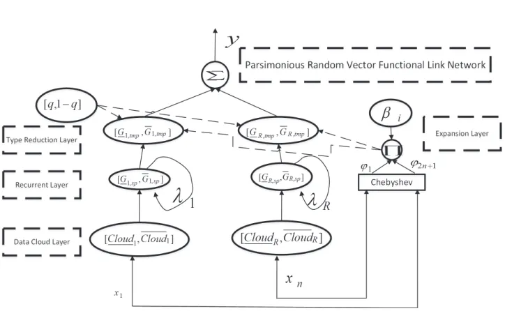
absence of self-organizing mechanism. The problem of uncertainty is another
143
open issue in the existing literature since most work utilises a crisp activation
144
function generating certain activation degrees. Such functions lack a degree
145
of tolerance against imprecision, inaccuracy and uncertainty in the training
146
data. It is worth noting that uncertainty occurs for a number of reasons:
147
noisy measurement, noisy data, false sensor reading, etc.
148
3. Basic Concepts 149
This section outlines the foundations of pRVFLN encompassing the basic
150
concept of RVFLN [17], the use of the Chebyshev polynomial as the
tional expansion block [23] and the concept of data clouds [24].
152
3.1. Random Vector Functional Link Network
153
The idea of RVFLN was proposed by Pao in [17] and is one of the forms of
154
the functional link network combined with the random vector approach [18].
155
It starts with the fact that while the network parameters are set as random
156
pairings of points, the training set can be still learned very well, although it
157
does not remove the inherent nature of random process. It features the
en-158
hancement node performing the nonlinear transformation of input attributes
159
as well as the direct connection of input attributes to the output node. The
160
activation degree of the enhancement node along with the input attributes
161
is combined with a set of output weights to generate the final network
out-162
put. The RVFLN only leaves the weight vector to be fine-tuned during the
163
training process while the other parameters are randomly sampled from a
164
carefully selected scope. Suppose that there are J enhancement nodes and
165
N input attributes, the size of the output weight vector isW ∈ <(J+N). The 166
quadratic optimization problem is then formulated as follows:
167
E = 1 2P
P X
p=1
(t(p)−Btd(p))2 (1)
where B ∈ <(N+J) is the output weight vector containing the N-dimensional
168
original input vector also in addition to the weight values. d(p) is the output
169
of the enhancement node. The RVFLN is similar to a single hidden layer
170
feedforward network except for the fact that the hidden node functions as an
171
enhancement of the input feature and there exists direct connection from the
172
input layer to the output layer. The steepest descent approach can be used to
173
fine-tune the output weight vector. If matrix inversion using pseudo-inverse
174
is feasible, a closed-form solution can be formulated. The generalization
175
performance of RVFLN was examined in [17] where RVFL can be trained
176
rapidly with ease. The RVFLNs convergence is also guaranteed to be attained
177
within a number of iterations.
178
The RVFL can be modified by incorporating the idea of the functional
179
link network [23]. That is, the hidden node or the enhancement node is
180
replaced by the functional expansion block generating a set of linearly
in-181
dependent functions of the entire input pattern. The functional expansion
182
block can be formulated as trigonometric expansion [25], Chebyshev
expan-183
sion, legendre expansion, etc. [23] but our scope of discussion is limited to
the Chebyshev expansion only due to its relevance to pRVFLN. Given theN
-185
dimensional input vector X = [x1, x2, ..., xN]∈ <1×N and its corresponding 186
m-dimensional target vector Y = [y1, y2, ..., ym]∈ <1×m, the output of RVFL 187
with the Chebyshev functional expansion block is expressed as follows:
188
y=
2N+1 X
j=1
Bjφj(ANXN +bN) (2)
where Bj is the output weight vector and φj() is the Chebyshev functional
189
expansion mapping the N-dimensional input attribute and the input weight
190
vector to the higher 2N + 1 expansion space. As with the original RVFLN,
191
the output weight vector can be learned using any optimization method. The
192
2N + 1 here results from the utilisation of the Chebyshev series up to the
193
second order. The Chebyshev series is mathematically written as follows:
194
Tn+1 = 2xTn(x)−Tn−1(x) (3)
If we are only interested in the Chebyshev series up to the second order,
195
this results in To(x) = 1, T1(x) = x, T2(x) = 2x2 −1. The advantage of the 196
Chebyshev functional link compared to other popular functional links such as
197
trigonometric [25], legendre, power function, etc. [23] lies in its simplicity of
198
computation. The Chebyshev function scatters fewer parameters to be stored
199
into memory than the trigonometric function, while the Chebyshev function
200
has a better mapping capability than the other polynomial functions of the
201
same order. In addition, the polynomial power function is not robust against
202
an extrapolation case.
203
3.2. Data Cloud
204
The concept of the data cloud offers an alternative to the traditional
205
cluster concept where it is not shape-specific and evolves naturally in
ac-206
cordance with the true data distribution. It is also easy to use because it
207
is non-parametric and does not require any parameterization. This
strat-208
egy is desirable because parameterization per scalar variable often calls for
209
complex high-level approximation and/or optimization. This approach was
210
inspired by the idea of RDE and was integrated in the context of the TSK
211
fuzzy system [11, 24]. Unlike a conventional fuzzy system where a degree
212
of membership is defined by a point-to-point distance, the data cloud
com-213
putes an accumulated distance of the point of interest to all other points in
the data cloud without physically keeping all data samples in the memory
215
similar to the local data density. This notion has a positive impact on the
216
memory and space complexity because the number of network parameters
217
significantly reduces. The data cloud concept is formally written as:
218
γki = 1
1 +||xk−µLk|| 2
+ ΣL
k − ||µLk||
2 (4)
whereγi
k denotes thei-th data cloud at thek-th observation. The data cloud
219
evolves by updating the local mean µLk and square length of i-th local region
220
ΣL
k as follows: 221
µLk = (M
i k−1 Mi
k
)µLk−1+ xk
Mi k
, µL1 =x1 (5)
222
ΣLk = M
i k−1 Mi
k
ΣLk−1 +||xk||
2
Mi k
,ΣL1 =||x1||2 (6)
It is worth noting that these two parameters correspond to statistics of the
223
i-th data cloud and are computed recursively with ease using standard
re-224
cursive formulas. They do not impose a specific optimization or a specific
225
setting to be performed to adjust their values.
226
4. Network Architecture of pRVFLN 227
pRVFLN utilises a local recurrent connection at the hidden node which
228
generates the spatiotemporal activation degree. This recurrent connection
229
is realized by a self-feedback loop of the hidden node which memorizes the
230
previous activation degree and outputs a weighted combination between
pre-231
vious and current activation degrees spatiotemporal firing strength. In the
232
literature, there exist at least three types of recurrent network structures
re-233
ferring to its recurrent connections: global [26, 27], interactive [25], and local
234
[28], but the local recurrent connection is deemed to be the most
compati-235
ble recurrent type in our case because it does not harm the local property,
236
which assures stability when adding, pruning and fine-tuning hidden nodes.
237
pRVFLN utilises the notion of the functional-link neural network where the
238
expansion block is created by the Chebyshev polynomial up to the second
239
order. Furthermore, the hidden layer of pRVFLN is built upon an
interval-240
valued data cloud [11] where we integrate the idea of an interval-valued local
241
mean into the data cloud.
Suppose that a pair of data points (Xt, Tt) is received att-th time instant 243
where Xt ∈ <n is an input vector and Tt ∈ <m is a target vector, while n 244
and m are respectively the number of input and output variables. Because
245
pRVFLN works in a strictly online learning environment, it has no access
246
to previously seen samples, and a data point is simply discarded after being
247
learned. Due to the pre-requisite of an online learner, the total number of
248
data N is assumed to be unknown. The output of pRVFLN is defined as
249
follows:
250
yo = R X
i=1
βiG˜i,temporal(AtXt+Bt),Getemporal= [G, G] (7)
where R denotes the number of hidden nodes and βi stands for the i-th
251
output of the functional expansion layer, produced by weighting the weight
252
vector with an extended input vector βi = xTewi. xe ∈ <(2n+1)×1 is an 253
extended input vector resulting from the functional link neural network based
254
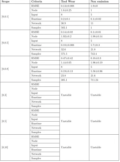
on the Chebyshev function up to the second order [23] as shown in (3) and
255
wi ∈ <(2n+1)×1 is a connective weight of the i-th output node. The definition 256
of βi is rather different from its common definition in the literature because
257
it adopts the concept of the expansion block, mapping a lower dimensional
258
space to a higher dimensional space with the use of certain polynomials. This
259
paradigm produces the extended input vector xe as follows:
260
νp+1(x) = 2xjνp(xj)−νp−1(xj) (8)
where ν0(xj) = 1, ν1(xj) = xj, ν2(xj) = 2x2j −1. Suppose that three input 261
attributes are givenX = [x1, x2, x3], the extended input vector is expressed as 262
the Chebyshev polynomial up to the second orderxe= [1, x1, ν2(x1), x2, ν2(x2), 263
x3, ν(x3)]. Note that the term 1 here represents an intercept of the output 264
node to avoid going through the origin, which may risk an untypical gradient.
265
At ∈ <n is an input weight vector randomly generated from a certain range. 266
Btis removed for simplicity. Gei,temporalis the i-th interval-valued data cloud, 267
triggered by the upper and lower data cloud Gi,temporal, Gi,temporal. Note that 268
recurrence is not seen in (7) because pRVFLN makes use of local recurrent
269
layers at the hidden node. By expanding the interval-valued data cloud [29],
270
the following is obtained:
271
yo = R X
i=1
(1−qo)βiGi,temporal+ R X
i=1
where q ∈ <m is a design factor to reduce an interval-valued function to a
crisp one [29]. It is worth noting that the upper and lower activation func-tions Gi,temporal, Gi,temporal deliver spatiotemporal characteristics as a result
of a local recurrent connection at the i-th hidden node, which combines the spatial and temporal firing strength of the i-th hidden node. These temporal activation functions output the following.
Gti,temporal =λiGti,spatial + (1−λi)Gti,temporal−1 , Gti,temporal=λiG
t
i,spatial+ (1−λi)G t−1
i,temporal (10)
where λ ∈ <R is a weight vector of the recurrent link. The local feedback
272
connection here feeds the spatiotemporal firing strength at the previous time
273
step Geti,temporal−1 back to itself and is consistent with the local learning princi-274
ple. This trait happens to be very useful in coping with the temporal system
275
dynamic because it functions as an internal memory component which
mem-276
orizes a previously generated spatiotemporal activation function at t −1.
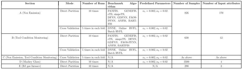
277
Also, the recurrent network is capable of overcoming over-dependency on
278
time-delayed input features and lessens strong temporal dependencies of
sub-279
sequent patterns. This trait is desired in practise since it may lower the input
280
dimension, because prediction is done based on the most recent measurement
281
only. Conversely, the feedforward network often relies on time-lagged input
282
attributes to arrive at a reliable predictive performance due to the absence
283
of an internal memory component. This strategy at least entails expert
284
knowledge for system order to determine the suitable number of delayed
285
components.
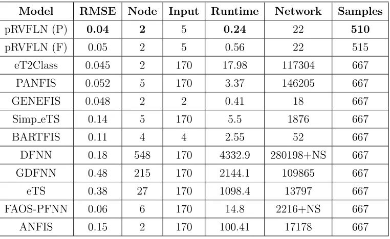
286
The hidden node of the pRVFLN is an extension of the cloud-based hidden
287
node, where it embeds an interval-valued concept to address the problem of
288
uncertainty [30]. Instead of computing an activation degree of a hidden node
289
to a sample, the cloud-based hidden node enumerates the activation degree
290
of a sample to all intervals in a local region on-the-fly. This results in local
291
density information, which fully reflects real data distributions. This concept
292
was defined in AnYa [11, 24]. This concept is also the underlying component
293
of AutoClass and TEDA-Class [31], all of which come from Angelovs sound
294
work of RDE [24]. This paper aims to modify these prominent works to the
295
interval-valued case. Suppose that Ni denotes the support of the i-th data
296
cloud, an activation degree ofi-th cloud-based hidden node refers to its local
density estimated recursively using the Cauchy function:
298
e
Gi,spatial =
1
1 +
Ni
P
k=1
(exk−xt
Ni )
, xek = [xk,i, xk,i], Gei,spatial = [Gi,spatial, Gi,spatial]
(11)
where xek is k-th interval in the i-th data cloud and xt is t-th data sample.
It is observed that (11) requires the presence of all data points seen so far. Its recursive form is formalised in [24] and is generalized here to the interval-valued case:
Gi,spatial =
1 1 +||AT
txt−µi,Ni||
2+ Σ
i,Ni − ||µi,Ni||
2,
Gi,spatial = 1
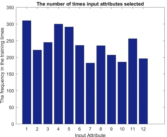
1 +||AT
txt−µi,N
i||
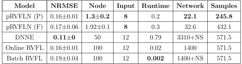
2+ Σ
i,Ni − ||µi,Ni||
2 (12)
where µ
i, µi signify the upper and lower local means of the i-th cloud:
µ
i,Ni = (
Ni−1 Ni
)µ
i,Ni−1+
xi,Ni −∆i ||Ni||
, µ
i,1 =xi,1−∆i,
µi,Ni = (Ni−1
Ni
)µi,Ni−1+
xi,k+ ∆i
||Ni,k||
, µi,1 =xi,1+ ∆i (13)
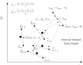
where ∆i is an uncertainty factor of the i-th cloud, which determines the
degree of tolerance against uncertainty. The uncertainty factor creates an interval of the data cloud, which controls the degree of tolerance for uncer-tainty. It is worth noting that a data sample is considered as a population of thei-th cloud when resulting in the highest density. Moreover, Σi,Ni,Σi,Ni
are the upper and lower mean square lengths of the data vector in the i-th
cloud as follows:
Σi,Ni = (Ni−1
Ni
)Σi,Ni−1+ ||xi,Ni||
2−∆ i
||Ni||
, Σi,1 =||xi,1||2−∆i,
Σi,Ni = (
Ni−1 Ni
)Σi,Ni−1+
||xi,Ni||
2+ ∆ i
||Ni||
, Σi,1 =||xi,1||2+ ∆i (14)
Although the concept of the cloud-based hidden node was generalized in
299
TeDaClass [32] by introducing the eccentricity and typicality criteria, the
300
interval-valued idea is uncharted in [32]. Note that the Cauchy function is
depicted in Fig. 1 and 2 respectively.
Fig. 1 Network Architecture of pRVFLN
Figure 1: Network Architecture of pRVFLN
asymptotically a Gaussian-like function, satisfying the activation function
302
requirement of the RVFLN to be a universal approximator.
303
Unlike conventional RVFLNs, pRVFLN puts into perspective a nonlinear
304
mapping of the input vector through the Chebyshev polynomial up to the
305
second order. Note that recently developed RVFLNs in the literature mostly
306
are designed with a zero-order output node [5, 6, 7, 8]. The functional
ex-307
pansion block expands the output node to a higher degree of freedom, which
308
aims to improve the local mapping aptitude of the output node. pRVFLN
309
implements the random learning concept of the RVFLN, in which all
pa-310
rameters, namely the input weight A, design factor q, recurrent link weight
311
λ, and uncertainty factor Delta, are randomly generated. Only the weight
312
vector is left for parameter learning scenario wi. Since the hidden node is
313
parameter-free, no randomization takes place for hidden node parameters.
314
The network structure of pRVFLN and the interval-valued data cloud are
315
depicted in Fig. 1 and 2 respectively.
316
5. Learning Policy of pRVFLN 317
This section discusses the learning policy of pRVFLN. Section 5.1
out-318
lines the online active learning strategy, which deletes inconsequential
sam-319
ples. Samples, selected in the sample selection mechanism, are fed into the
learning process of pRVFLN. Section 5.2 deliberates the hidden node growing
321
strategy of pRVFLN. Section 5.3 elaborates the hidden node pruning and
re-322
call strategy, while Section 5.4 details the online feature selection mechanism.
323
Section 5.5 explains the parameter learning scenario of pRVFLN. Algorithm
324
1 shows the pRVFLN learning procedure.
325
5.1. Online Active Learning Strategy
326
The active learning component of the pRVFLN is built on the extended
327
sequential entropy (ESEM) method, which is derived from the SEM method
328
[12]. The ESEM method makes use of the entropy of the neighborhood
prob-329
ability to estimate the sample contribution. The underlying difference from
330
its predecessor [12] lies in the integration of the data cloud paradigm, which
331
greatly relieves the effort in finding the neighborhood probability because the
332
data cloud itself is inherent with the local data density, taking into account
333
the influence of all samples in a local region. Furthermore, it handles the
334
regression problem which happens to be more challenging than the
classifi-335
cation problem because the sample contribution is estimated in the absence
336
of a decision boundary. To the best of our knowledge, only Das et al. [33]
337
address the regression problem, but they still employ a fully supervised
tech-338
nique because their method depends on the hinge error function to evaluate
339
the sample contribution. The concept of neighborhood probability refers to
340
the probability of an incoming data stream sitting in the existing data clouds:
341
P(Xi ∈Ni) = Ni
P
k=1
M(Xt,xk)
Ni
R P
i=1 Ni
P
k=1
M(Xt,xk)
Ni
(15)
where XT is a newly arriving data point andxn is a data sample, associated
342
with the i-th rule. M(XT,xk) stands for a similarity measure, which can
343
be defined as any similarity measure. The bottleneck is however caused by
344
the requirement to revisit already seen samples. This issue can be tackled
345
by formulating the recursive expression of (15). In the context of the data
346
cloud, this issue becomes even simpler, because it is derived from the idea
347
of local density and is computed based on the local mean [11]. (15) is then
348
written as follows:
349
P(Xi ∈Ni) =
Λi R P
i=1
Λi
where Λi is a type-reduced activation degree Λi = (1−q)Gi,spatial+qGi,spatial. 350
Once the neighbourhood probability is determined, its entropy is formulated
351
as follows:
352
H(N|Xi) =− R X
i=1
P(Xi ∈Ni)logP(Xi ∈Ni) (17)
Algorithm 1. Learning Architecture of pRVFLN
Algorithm 1: Parsimonious Random Vector Functional Link Net-work
Given a data tuple at t −th time instant (Xt, Tt) = (x1, ..., xn, t1, ..., tm), Xt∈ <n, Tt∈ <Rm; set predefined parameters α1, α2
/*Step 1: Online Active Learning Strategy/* For i=1 to R do
Calculate the neighborhood probability (8) with spatial firing strength (4) End For
Calculate the entropy of neighborhood probability (8) and the ESEM (10) IF (34) Then
/*Step 2: Online Feature Selection/* IF Partial=Yes Then
Execute Algorithm 3 Else IF
Execute Algorithm 2 End IF
/*Step 3: Data Cloud Growing Mechanism/* For j=1 to n do
Compute ξ(xj, T0) End For
For i=1 to R do
Calculate input coherence (12) For o=1 to m do
Calculate ξ(µei, T0) End For
/*Step 4: Data Cloud Pruning Mechanism/* For i=1 to R do
For o=1 to m do Calculate ξ(Gei,temp, T0) End For
IF (19) Then
Discard i-th data cloud End IF
End For
/*Step 5: Adaptation of Output Weight/* For i=1 to R do
Update output weights using FWGRLS End For
The entropy of the neighbourhood probability measures the uncertainty
355
induced by a training pattern. A sample with high uncertainty should be
356
admitted for the model update, because it cannot be well-covered by an
357
existing network structure and learning such a sample minimises uncertainty.
358
A sample is to be accepted for model updates, provided that the following
359
condition is met:
360
H ≥thres (18)
wherethresis an uncertainty threshold. This parameter is not fixed
dur-361
ing the training process, rather it is dynamically adjusted to suit the learning
362
context. The threshold is set as thresN+1 = thesN(1±inc), where it
aug-363
ments thresN+1 =thesN(1 +inc) when a sample is admitted for the training
364
process, whereas it decreases thresN+1 = thesN(1−inc) when a sample is
365
ruled out for the training process. inc here is a step size, set at inc = 0.01.
366
This simply follows its default setting in [21].
367 368
5.2. Hidden Node Growing Strategy
369
pRVFLN relies on the T2SCC method to grow interval-valued data clouds
370
on demand. This notion is extended from the so-called SCC method [14, 13]
371
to adapt to the type-2 hidden node working framework. The significance of
372
the hidden nodes in pRVFLN is evaluated by checking its input and output
373
coherence through an analysis of its correlation to existing data clouds and
374
the target concept. Let µei = [µi, µi] ∈ <1
×n be a local mean of the i-th
375
interval-valued data cloud (5),Xt ∈ <n is an input vector and Tt ∈ <n is a 376
target vector, the input and output coherence are written as follows:
377
Ic(˜µi, Xt) = (1−q)ζ(µi, Xt) +qζ(µi, Xt) (19)
378
Oc(˜µi, Xt) = (ζ(Xt, Tt)−ζ(˜µi, Tt)), ζ(˜µi, Tt) = (1−q)ζ(µi, Tt) +qζ(µi, Tt)
(20)
where ζ() is the correlation measure. Both linear and non-linear correlation
problems and it is used in the T2SCC to perform the correlation measure
ζ()[34]:
ζ(X1, X2) =
1
2(var(X1) + var(X2)
−p(var(X1) + var(X2))2−4var(X1)var(X2)(1−ρ(X1, X2)2))
(21)
ρ(X1, X2) =
cov(X1, X2) p
var(X1)var(X2)
(22)
where (X1, X2) are substituted with (µi, Xt),(µt, Xt),(µi, Tt),(µt, Tt),(Xt, Tt) 379
to calculate the input and output correlation (19), (20). respectively stand
380
for the variance of X, covariance of X1 and X2, and Pearson correlation
381
index of X1 and X2. The local mean of the interval-valued data cloud
rep-382
resents a data cloud because it represents a point with the highest density.
383
In essence, the MCI method indicates the amount of information
compres-384
sion when ignoring a newly observed sample. The MCI method features
385
the following properties: 1) 0 ≤ ζ(X1, Y2) ≤ 0.5(var(X1) + var(X2)), 2) 386
a maximum correlation is given by ζ(X1, X2) = 0, 3) a symmetric
prop-387
erty ζ(X1, X2) = ζ(X2, X1), 4) it is invariant against the translation of the 388
dataset, and 5) it is also robust against rotation.
389
The input coherence explores the similarity between new data and
ex-390
isting data clouds directly, while the output coherence focusses on their
dis-391
similarity indirectly through a target vector as a reference. The input and
392
output coherence formulates a test that determines the degree of confidence
393
in the current hypothesis:
394
Ic(˜µi, Xt)≤α1, Oc(˜µi, Xt)≥α2 (23)
where α1 ∈ [0.001,0.01], α2 ∈ [0.01,0.1] are predefined thresholds. If a hy-395
pothesis meets both conditions, a new training sample is assigned to a data
396
cloud with the highest input coherence i∗. Accordingly, the number of
in-397
tervals N i∗, local mean and square length ˜µi∗,Σ˜i∗ are updated respectively
398
with (21) and (22) as well as Ni∗ =Ni∗+ 1. A new data cloud is introduced,
399
provided that the existing hypotheses do not pass either condition (23) , that
400
is, one of the conditions is violated. This situation reflects the fact that a new
401
training pattern conveys significant novelty, which has to be incorporated to
402
enrich the scope of the current hypotheses. Note that if a larger α1 is
spec-403
ified, fewer data clouds are generated and vice versa, whereas if a larger α2
t is also robust against rotation.
Figure 2: Interval Valued Data Cloud
is specified, larger data clouds are added and vice versa. The sensitivity of
405
these two parameters is studied in the section V.E of this paper. Because a
406
data cloud is non-parametric, no parameterization is committed when adding
407
a new data cloud. The output node of a new data cloud is initialised:
408
WR+1 =Wi∗, ΨR+1 =ωI (24)
where ω = 105 is a large positive constant. The output node is set as the
409
data cloud with the highest input coherence because this data cloud is the
410
closest one to the new data cloud. Furthermore, the setting of covariance
411
matrix ΨR+1 leads to a good approximation of the global minimum solution
412
of batched learning, as proven mathematically in [35].
413
5.3. Hidden Node Pruning and Recall Strategy
414
pRVFLN incorporates a data cloud pruning scenario, termed the
type-415
2 relative mutual information (T2RMI) method. This method was firstly
developed in [36] for the type-1 fuzzy system. This method is convenient to
417
apply here because it estimates mutual information between a data cloud and
418
a target concept by analysing their correlation. Hence, the MCI method (21),
419
(22) is valid to measure the correlation between two variables. Although this
420
method has been well-established [36], to date, its effectiveness in handling
421
data clouds and a recurrent structure as implemented in pRVFLN is an open
422
question. Unlike both the RMI method that applies the classic symmetrical
423
uncertainty method, the T2RMI method is formalised using the MCI method
424
as follows:
425
ζ( ˜Gi,temp, Tt) = qζ(Gi,temp, Tt) + (1−q)ζ(Gi,temp, Tt) (25)
where Gi,temp, overlineGi,temp are respectively the lower and upper
tempo-426
ral activation functions of the i-th rule. The temporal activation function
427
is included in (25) rather than the spatial activation function in order to
428
account for the inter-temporal dependency of subsequent training samples.
429
The MCI method is chosen here because it possesses a significantly lower
430
computational burden than the symmetrical uncertainty method but it is
431
still more robust than a linear Pearson correlation index. A data cloud is
432
deemed inconsequential, if the following is met:
433
ζi < mean(ζi)−2std(ζi) (26)
where mean(ζi), std(ζi) are respectively the mean and standard deviation 434
of the MCI during its lifespan. This criterion aims to capture an obsolete
435
data cloud which does not keep up with current data distribution due to
436
possible concept drift, because it computes the downtrend of the MCI values
437
during its lifespan. It is worth mentioning that mutual information between
438
hidden nodes and the target variable is a reliable indicator for changing data
439
distributions because it monitors significance of a local region with respect
440
to the recent data context.
441
The T2RMI method also functions as a rule recall mechanism to cope with
442
cyclic concept drift. Cyclic concept drifts frequently happen in relation to the
443
weather, customer preferences, electricity power consumption problems, etc.
444
all of which are related to seasonal change. This points to a situation where
445
a previous data distribution reappears in the current training step. Once
446
pruned by the T2RMI, a data cloud is not forgotten permanently and is
447
inserted into a list of pruned data clouds R∗ =R∗+ 1. In this case, its local
448
mean, square length, population, an output node, and output covariance
matrix ˜µR∗,Σ˜R∗, NR∗, βR∗,ΨR∗, are retained in memory. Such data clouds
450
can be reactivated in the future, whenever their validity is confirmed by an
451
up-to-date data trend. It is worth noting that adding a completely new data
452
cloud when observing a previously learned concept catastrophically erases the
453
learning history. A data cloud is recalled subject to the following condition:
454
max(ζi∗)
i∗=1,...,R∗
>max(ζi) i=1,...,R
(27)
This situation reveals that a previously pruned data cloud is more relevant
455
than any existing ones. This condition pinpoints that a previously learned
456
concept reappears again. A previously pruned data cloud is then regenerated
457
as follows:
458
˜
µR+1 = ˜µR∗,Σ˜R+1 = ˜ΣR∗, NR+1 =NR∗, βR+1 =βR∗,ΨR+1 = ΨR∗ (28)
Although previously pruned data clouds are stored in memory, all previously
459
pruned data clouds are excluded from any training scenarios except (18).
460
Unlike its predecessors [10], this rule recall scenario is completely independent
461
from the growing process (please refer to Algorithm 1).
462
5.4. Online Feature Selection Strategy
463
A prominent work, namely online feature selection (OFS), was developed
464
in [15]. The appealing trait of OFS lies in its aptitude for flexible feature
465
selection, as it enables the provision of different combinations of input
at-466
tributes in each episode by activating or deactivating input features (1 or 0)
467
in accordance to the up-to-date data trend. Furthermore, this technique is
468
also capable of handling partial input attributes which are fruitful when the
469
cost of feature extraction is too expensive. OFS is generalized here to fit the
470
context of pRVFLN and to address the regression problem.
471
We start our discussion from a condition where a learner is provided with
472
full input variables. Suppose that B input attributes are to be selected in
473
the training process andB < n, the simplest approach is to discard the input
474
features with marginal accumulated output weights
R P
i=1 2 P
j=1
βi,j and maintain
475
onlyB input features with the largest output weights. Note that the second
476
term
2 P
j=1
is required because of the extended input vector xe ∈ <(2n+1). The 477
rule consequent informs a tendency or orientation of a rule in the target space
which can be used as an alternative to gradient information [35]. Although it
479
is straightforward to use, it cannot ensure the stability of the pruning process
480
due to a lack of sensitivity analysis of the feature contribution. To correct
481
this problem, a sparsity property of the L1 norm can be analyzed to
exam-482
ine whether the values of n input features are concentrated in the L1 ball.
483
This allows the distribution of the input values to be checked to determine
484
whether they are concentrated in the largest elements and that pruning the
485
smallest elements wont harm the models accuracy. This concept is actualized
486
by first inspecting the accuracy of pRVFLN. The input pruning process is
487
carried out when the system error is large enough Tt−yt > κ. Nevertheless, 488
the system error is not only large in the case of underfitting, but also in
489
the case of overfitting. We modify this condition by taking into account the
490
evolution of system error |et+σt|> κ|et−1 +σt−1| which corresponds to the 491
global error mean and standard deviation. The constant κ is a predefined
492
parameter and fixed at 1.1. The output nodes are updated using the gradient
493
descent approach and then projected to the L2 ball to guarantee a bounded
494
norm. Algorithm 2 details the algorithmic development of pRVFLN.
495
496
Algorithm 2. GOFS using full input attributes
Input: α learning rate, χ regularization factor, B the number of features to be retained
Output: selected input features Xt,selected ∈ <1×B For t=1,., T
Make a prediction yt
IF |et+σt|>1.1|et−1+σt−1| // for regression ˆo = max
o=1,...,m(yo)6=Tt or //
for classification
βi =βi−χα βi−αχ∂β∂Ei, βi = min(1, 1/√χ
||βi||2)βi
Prune input attributes Xt except those of B largest
R P
i=1 2 P
j=1 βi,j
Else
βi =βi−χαβi End IF End FOR 497
498
whereα, χare respectively the learning rate and regularization factor. We
499
assign α = 0.2, χ = 0.01 following the same setting [15]. The optimization
500
procedure relies on the standard mean square error (MSE) as the objective
function and utilises the conventional gradient descent scenario:
502
∂E ∂βi
= (Tt−yt)
( R
X
i=1
(1−q)Gi,temporal+ R X
i=1
qGi,temporal )
(29)
Furthermore, the predictive error has been theoretically proven to be bounded
503
in [17] and the upper bound is also found. One can also notice that the GOFS
504
enables different feature subsets to be elicited in each training observation t.
505
A relatively unexplored area of existing online feature selection is a
situa-506
tion where a limited number of features is accessible for the training process.
507
To actualise this scenario, we assume that at most B input variables can
508
be extracted during the training process. This strategy, however, cannot be
509
done by simply acquiring any B input features, because this scenario risks
510
having the same subset of input features during the training process. This
511
problem is addressed using the Bernaoulli distribution with confidence level
512
to sample B input attributes from n input attributes B < n. Algorithm 3
513
displays the feature selection procedure.
514
Algorithm 3. GOFS using partial input attributes
Input: α learning rate, χ regularization factor, B the number of features
to be retained, confidence level
Output: selected input features Xt,selected ∈ <1×B For t=1,., T
Sample γ from Bernaoulli distribution with confidence level
IF γt= 1
Randomly select B out of n input attributesXet∈ <1×B End IF
Make a prediction yt
IF |et+σt|>1.1|et−1+σt−1| // for regression ˆo = max
o=1,...,m(yo)6=Tt or //
for classification ˆ
Xt=Xet
(B/n) + (1−)
βi =βi−χα βi−αχ∂β∂Ei, βi = min(1, 1√χ
||βi||2)βi
Prune input attributes Xt except those of B largest
R P
i=1 2 P
j=1 βi,j
Else βi,t =βi,t−1 End IF End FOR 516
517
As with Algorithm 2, the convergence of this scenario has been
theoreti-518
cally proven and the upper bound is derived in [17]. One must bear in mind
519
that the pruning process in Algorithm 1 and 2 is carried out by assigning
520
crisp weights (0 or 1), which fully reflect the importance of the input features.
521
5.5. Random Learning Strategy
522
pRVFLN adopts the random parameter learning scenario of the RVFLN,
523
leaving only the output nodes W to be analytically tuned with an online
524
learning scenario, whereas others, namely At, q, λ,∆, can be randomly
gen-525
erated without any tuning process. To begin the discussion, we recall the
526
output expression of pRVFLN as follows:
527
yo= R X
i=1
Referring to the RVFLN theory, the activation function ˜Gi,spatial should be 528
either integrable or differentiable:
529
Z
R
G2(x)dx <∞, or Z
R
[G0(x)]2dx <∞ (31)
Furthermore, a large number of hidden nodes R is usually needed to ensure
530
adequate coverage of data space because hidden node parameters are chosen
531
at random [37]. Nevertheless, this condition can be relaxed in the pRVFLN,
532
because the data cloud growing mechanism, namely the T2SCC method,
533
partitions the input region in respect to real data distributions. The data
534
cloud-based neurons are parameter-free and thus do not require any
param-535
eterization, which often calls for a high-level approximation or complicated
536
optimization procedure. Other parameters, namely At, q, λ,∆, are randomly
537
chosen, and their region of randomisation should be carefully selected.
Re-538
ferring to [38], the parameters are sampled randomly from the following.
539
b=−w0y0−µ0
w0 =αw0; w0 ∈[0; Ω]×[−Ω; Ω]d−1 y0 ∈Id
µ0 ∈[−2dΩ,2dΩ]
(32)
where u,Ω, α are probability measures. Nevertheless, this strategy is
im-540
possible to implement in online situations because it often entails a rigorous
541
trial-error process to determine these parameters. Most RVFLNs work
sim-542
ply by following Schmidt et al.s strategy [9], that is, setting the region of
543
random parameters in the range of [-1,1].
544
Assuming that a complete dataset Ξ = [X, T]∈ <N×(n+m)is observable, a 545
closed-form solution of (23) can be defined to determine the output weights .
546
Although the original RVFLN adjusts the output weight with the conjugate
547
gradient (CG) method, the closed-form solution can still be utilised with
548
ease [4]. The obstacle for the use of pseudo-inversion in the original work
549
was the limited computational resources in 90’s. Although it is easy to use
550
and ensures a globally optimum solution, this parameter learning scenario
551
however imposes revisiting preceding training patterns which are intractable
552
for online learning scenarios. pRVFLN employs the FWGRLS method [39]
553
to adjust the output weight. As the FWGRLS approach has been detailed
554
in [39], it is not recounted here.
Table 2: Details of Experimental Procedure
Section Mode Number of Runs Benchmark Algo-rithm
Predefined Parameters Number of Samples Number of Input attributes
A (Nox Emission) Direct Partition 10 times PANFIS,eTS, simpeTS,GENEFIS, DFNN, GDFNN, FAOS-PFNN, ANFIS, BART-FIS
α1= 0.002, α2= 0.02
826 170
Cross Validation 5 times in each fold DNNE, OnlineRVFL, Batch RVFL
α1= 0.002, α2= 0.02
B (Tool Condition Monitoring) Direct Partition 10 times PANFIS,eTS, simpeTS, DFNN,GENEFIS, GDFNN, FAOS-PFNN, ANFIS, BARTFIS
α1= 0.002, α2= 0.02
630 12
Cross Validation 5 times in each fold DNNE, OnlineRVFL, Batch RVFL
α1= 0.002, α2= 0.02
C (Nox Emission, Tool Condition Monitoring) Cross Validation 5 times in each fold N/A α1= 0.002, α2= 0.02 As above As above D (Mackey Glass) Direct Partition 10 times N/A α1= 0.002, α2= 0.02 3500 4
E (BJ gas furnace) Direct Partition 10 times N/A N/A 290 2
5.6. Robustness of RVFLN
556
The network parameters are usually sampled uniformly within a range of
557
[-1,1] in the literature. A new finding of Li and Wang in [22] exhibits that
558
randomly generating network parameters with a fixed scope [−α, α] does not
559
ensure a theoretically feasible solution or often the hidden node matrix is
560
not full rank. Surprisingly, the hidden node matrix was not invertible in all
561
their case studies when randomly sampling network parameters in the range
562
of [-1,1] and far better numerical results were achieved by choosing the scope
563
[-200,200]. This trend was consistent with different numbers of hidden nodes.
564
How to properly select scopes of random parameters and its corresponding
565
distribution still require in-depth investigation [9]. In practice, a pre-training
566
process is normally required to arrive at a decent scope of random parameters.
567
Note that the range of random parameters by Igelnik and Pao [4] is still at
568
the theoretical level and does not touch the implementation issue. We study
569
different random regions in Section 5.5 to see how pRVFLN behaves under
570
variations of the scope of random parameters.
571
6. Numerical Examples 572
This section presents the numerical validation of our proposed algorithm
573
using case studies and comparisons with prominent algorithms in the
litera-574
ture. Two numerical examples, namely modelling of Nox emissions from a car
575
engine and tool condition monitoring in the ball-nose end milling process, are
576
presented in this section, and the other three numerical examples are placed
577
in the supplemental document 1 to keep the paper compact. Our numerical
578
Table 3: Prediction of Nox emissions Using Time-Series Mode
Model RMSE Node Input Runtime Network Samples
pRVFLN (P) 0.04 2 5 0.24 22 510
pRVFLN (F) 0.05 2 5 0.56 22 515
eT2Class 0.045 2 170 17.98 117304 667
PANFIS 0.052 5 170 3.37 146205 667
GENEFIS 0.048 2 2 0.41 18 667
Simp eTS 0.14 5 170 5.5 1876 667
BARTFIS 0.11 4 4 2.55 52 667
DFNN 0.18 548 170 4332.9 280198+NS 667
GDFNN 0.48 215 170 2144.1 109865 667
eTS 0.38 27 170 1098.4 13797 667
FAOS-PFNN 0.06 6 170 14.8 2216+NS 667
ANFIS 0.15 2 170 100.41 17178 667
studies were carried out under two scenarios: the time-series scenario and the
579
cross-validation (CV) scenario. The time-series procedure orderly executes
580
data streams according to their arrival and partitions data streams into two
581
parts, namely training and testing. Simulations were repeated 10 times and
582
numerical results were averaged from 10 runs to arrive at conclusive findings.
583
In the time-series mode, pRVFLN was compared against 10 state-of-the-art
584
evolving algorithms: eT2Class [40], BARTFIS [41], PANFIS [42], GENEFIS
585
[43], eTS [44], simp eTS [45], DFNN [46], GDFNN [47], FAOSPFNN [48],
586
ANFIS [49]. The CV scenarios were taken place in our experiment in order
587
to follow the commonly adopted simulation environment of other RVFLNs in
588
the literature where five runs per each fold were undertaken. pRVFLN was
589
benchmarked against the decorelated neural network ensemble (DNNE) [5],
590
online and batch versions of RVFL [9]. The pRVFLN MATLAB codes are
591
provided in 2 while the MATLAB codes of DNNE and RVFL are available
592
online3,4. Comparisons were performed against five evaluation criteria:
accu-593
2https://www.dropbox.com/sh/zbm54epk8trlnq9/AACgxLHt5Nsy7MISbgXcdkTba?dl=0
3http://homepage.cs.latrobe.edu.au/dwang/html/DNNEweb/index.html
Table 4: Prediction of Nox emissions Using CV Mode
Model NRMSE Node Input Runtime Network Samples
pRVFLN (P) 0.12±0.04 2 5 1.1 22 699 pRVFLN (F) 0.12±0.03 2 5 5.98 22 630.7
DNNE 0.14±0 50 170 0.81 43600+NS 744 Online RVFL 0.52±0.02 100 170 0.03 87200 744 Batch RVFL 0.59±0.05 100 170 0.003 87200+NS 744
racy, data clouds, input attribute, runtime, network parameters. The scope
594
of random parameters followed Schmidt’s suggestion [9] where the scope of
595
random parameters was [-1,1] but we insert the analysis of robustness in
596
part C which provides additional results with different random regions and
597
illustrates how the scope of random parameters influences the final numerical
598
results. The effect of the individual learning component to the end results and
599
the influence of user-defined predefined thresholds are analysed in Section D
600
and E. Furthermore, additional numerical results across different problems
601
are provided in the supplemental document 1. To allow a fair comparison, all
602
consolidated algorithms were executed in the same computational resources
603
under the MATLAB environment. Details of the experimental procedure are
604
tabulated in Table 2.
605
6.1. Modeling of Nox Emissions from a Car Engine
606
This section demonstrates the efficacy of the pRVFLN in modeling Nox
607
emissions from a car engine [50]. This real-world problem is relevant to
608
validate the learning performance, not only because it features noisy and
609
uncertain characteristics similar to the nature of a car engine, it also
char-610
acterizes high dimensionality, containing 170 input attributes. That is, 17
611
physical variables were captured in 10 consecutive measurements.
Further-612
more, different engine parameters were applied to induce changing the system
613
dynamics to simulate real driving actions across different road conditions. In
614
the time-series procedure, 826 data points were streamed to consolidated
al-615
gorithms, where 667 samples were set as training samples, and the remainder
616
were fed for testing purposes. 10 runs were carried out to attain consistent
617
numerical results. In the CV procedure, the experiment was run under the
618
10-fold CV, and each fold was repeated five times similar to the scenario
619
adopted in [26]. This strategy checks the consistency of the RVFLNs
learn-620
ing performance because it adopts the random learning scenario and avoids
621
data order dependency. Table 3 and 4 exhibit the consolidated numerical
622
results of benchmarked algorithms.
[image:29.612.115.501.245.484.2]623
Table 5: Tool Wear Prediction Using Time Series Mode
Model RMSE Node Input Runtime Network Samples
pRVFLN (P) 0.14 2 8 0.34 34 157
pRVFLN (F) 0.19 2 8 0.15 34 136
eT2Class 0.16 4 12 1.1 1260 320
Simp eTS 0.22 17 12 1.29 437 320
eTS 0.15 7 12 0.56 187 320
BARTFIS 0.16 6 12 0.43 222 320
PANFIS 0.15 3 12 0.77 507 320
GENEFIS 0.13 42 12 0.88 507 320
DFNN 0.27 42 12 2.41 1092+NS 320
GDFNN 0.26 7 12 2.54 259+ NS 320
FAOS-PFNN 0.38 7 12 3.76 1022+NS 320
ANFIS 0.16 8 12 0.52 296+ NS 320
Table 6: Tool wear prediction using CV Mode
Model NRMSE Node Input Runtime Network Samples
pRVFLN (P) 0.16±0.01 1.3±0.2 8 0.2 22.1 245.8
pRVFLN (F) 0.17±0.06 1.92±0.1 8 0.3 32.6 432.1 DNNE 0.11±0 50 12 0.79 3310+NS 571.5 Online RVFL 0.16±0.01 100 12 0.02 1400 571.5 Batch RVFL 0.19±0.04 100 12 0.002 1400+NS 571.5
It is evident that pRVFLN outperformed its counterparts in all the
evalua-624
tion criteria except GENEFIS for the number of input attributes and network
[image:29.612.111.498.530.633.2]parameters. It is worth mentioning however that in the other three criteria:
626
predictive accuracy, execution time, and number of training samples, the
627
GENEFIS was inferior to ours. pRVFLN is equipped with an online active
628
learning strategy, which discards superfluous samples. This learning
mod-629
ule had a significant effect on predictive accuracy. Furthermore, pRVFLN
630
utilizes the GOFS method, which is capable of coping with the curse of
di-631
mensionality. Note that the unique feature of the GOFS method is that
632
it allows different feature subsets to be picked up in every training episode
633
which avoids the catastrophic forgetting of obsolete input attributes,
tem-634
porarily inactive due to changing data distributions. The GOFS can handle
635
partial input attributes during the training process and results in the same
636
level of accuracy as that of the full input attributes. The use of full input
637
attributes slowed down the execution time because it needed to deal with
638
170 input variables first, before reducing the input dimension. In this case
639
study, we selected five input attributes to be kept for the training process.
640
Our experiment showed that the number of selected input attributes is not
641
problem-dependent and is able to be set as any desirable number in most
642
cases. We did not observe significant performance difference when using
ei-643
ther the full input mode or partial input mode. On the other hand, consistent
644
numerical results were achieved by pRVFLN, although the pRVFLN is built
645
on the random vector functional link algorithm, as observed in the CV
ex-646
perimental scenario. In addition, pRVFLN produced the most encouraging
647
performance in almost all evaluation criteria except computational speed
be-648
cause other RVFLNs implement less comprehensive training procedures than
649
pRVFLN. Note that although DNNE attained the highest accuracy in the
650
CV mode, it imposed considerable memory and space complexities.
651
6.2. Tool Condition Monitoring of High-Speed Machining Process
652
this section presents a real-world problem from a complex manufacturing
653
process (Courtesy of Dr. Li Xiang, Singapore) [51]. The objective of this
654
case study is to perform predictive analytics of the tool wear in the
ball-655
nose end milling process frequently found in the metal removal process of
656
the aerospace industry. In total, 12 time-domain features were extracted
657
from the force signal and 630 samples were collected during the experiment.
658
Concept drift in this case study resulted from changing surface integrity,
659
tool wear degradation as well as varying machining configurations. For the
660
time-series experimental procedure, the consolidated algorithms were trained
661
using data from cutter A, while the testing phase exploited data from cutter
Figure 3: The frequency of input features
B. This process was repeated 10 times to achieve valid numerical results.
663
For the CV experimental procedure, the 10-fold CV process was undertaken
664
where each fold was undertaken five times to arrive at consistent findings.
665
Tables 5 and 6 report the average numerical results across all folds. Fig. 3
666
depicts how many times input attributes are selected during one fold of the
667
CV process.
668
It is observed from Table 5 and 6 that pRVFLN evolved the lowest
struc-669
tural complexities while retaining a high accuracy. It is worth noting that
670
although the DNNE exceeded pRVFLN in accuracy, it imposed considerable
671
complexity because it is an offline algorithm revisiting previously seen data
672
samples and adopts an ensemble learning paradigm. The efficacy of the
on-673
line sample selection strategy was seen, as it led to a significant reduction of
674
training samples to be learned during the experiment. Using partial input
675
information led to subtle differences to those with the full input information.
676
It is seen in Fig. 3 that the GOFS selected different feature subsets in
ev-677
ery training episode. Additional numerical examples, sensitivity analysis of