Understanding the thermal properties of amorphous solids using machine learning based interatomic potentials

Original citation:

Sosso, Gabriele C., Deringer, Volker L., Elliott, Stephen R. and Csányi , Gábor (2018) Understanding the thermal properties of amorphous solids using machine-learning-based interatomic potentials. Molecular Simulation . doi:10.1080/08927022.2018.1447107

Permanent WRAP URL:

http://wrap.warwick.ac.uk/100416

Copyright and reuse:

The Warwick Research Archive Portal (WRAP) makes this work by researchers of the University of Warwick available open access under the following conditions. Copyright © and all moral rights to the version of the paper presented here belong to the individual author(s) and/or other copyright owners. To the extent reasonable and practicable the material made available in WRAP has been checked for eligibility before being made available.

Copies of full items can be used for personal research or study, educational, or not-for-profit purposes without prior permission or charge. Provided that the authors, title and full

bibliographic details are credited, a hyperlink and/or URL is given for the original metadata page and the content is not changed in any way.

Publisher’s statement:

“This is an Accepted Manuscript of an article published by Taylor & Francis in Molecular Simulation on 13/03/2018, available

online: http://www.tandfonline.com/10.1080/08927022.2018.1447107

.”

A note on versions:

The version presented here may differ from the published version or, version of record, if you wish to cite this item you are advised to consult the publisher’s version. Please see the ‘permanent WRAP URL’ above for details on accessing the published version and note that access may require a subscription.

Vol. 00, No. 00, Month 20XX, 1–26

Understanding the Thermal Properties of Amorphous Solids Using Machine-Learning-Based Interatomic Potentials

Gabriele C. Sossoa∗

a _{Department of Chemistry and Centre for Scientific Computing, University of Warwick, Gibbet Hill Road,}

Coventry CV4 7AL, United Kingdom

Volker L. Deringer,b,c _{Stephen R. Elliott,}c _{G´abor Cs´anyi}b

b_{Department of Engineering, University of Cambridge, Cambridge CB2 1PZ, United Kingdom} c_{Department of Chemistry, University of Cambridge, Cambridge CB2 1EW, United Kingdom}

(Received 00 Month 20XX; final version received 00 Month 20XX)

Understanding the thermal properties of disordered systems is of fundamental importance for condensed-matter physics—and it is of great relevance for practical applications as well. The manufacturing of window glass, the performance degradation of fiber-optics and the scalability of next-generation phase-change memories all depend on the thermal properties of amorphous solids. Whilemacroscopicproperties such as the thermal conductivity are usually well-characterised experimentally, theirmicroscopicorigin is often largely unknown. This is because the thermal properties of amorphous solids are determined by their vibrational (and possibly electronic) properties, which in turn depend upon the atomic-level structure. Hence there is a pressing need for atomistic simulations, which can in principle unravel the connection between microscopic structure and functional properties such as thermal conductivity. However, the large (long) length (time) scales involved are usually well beyond the reach ofab initiocalculations. On the other hand, many interesting amorphous materials are characterised by a very complex structure. This often prevents the construction of classical interatomic potentials which would enable simulations on much larger (longer) length (time) scales – if compared to those achievable by first-principles simulations. One way to get past this deadlock is to harness machine-learning (ML) algorithms to build interatomic potentials: these can be nearly as computationally efficient as classical force fields for molecular dynamics simulations while retaining much of the accuracy of first-principles calculations. Here, we discuss the contribution of these ML-based potentials to our understanding of the thermal properties of amorphous solids. We focus on neural-network potentials (NNPs) and Gaussian approximation potentials (GAPs), two of the most widespread theoretical frameworks available to date. We review the work that has been devoted to investigate, via NNPs, the thermal properties of phase-change materials, a class of systems widely used in the context of non-volatile memories. In addition, we present recent results on the vibrational properties of amorphous carbon, studied via GAPs. In light of these results, we argue that ML-based potentials are among the best options available to further our understanding of the vibrational and thermal properties of complex amorphous solids.

Keywords:neural networks; Gaussian approximation potential (GAP) models; thermal conductivity; phase-change materials; amorphous carbon

1. Introduction

The thermal properties of disordered solids are a problem of great interest in solid-state physics and materials science [1–6]. Many quantities of practical relevance, such as the thermal conductivity of a material, are largely determined by the underlying vibrational properties [7–9]. In crystals, which exhibit periodic long-range order, the vibrational excitations are likewise periodic and described by

a) b)

Vibrons

Extendons Locons

(localised vibrations)

(extended vibrations)

wavelength > mean free path

wavelength < mean free path

Energy

Vibrational density of states

Propagons Diffusons

mobility edge

Ioffe–Regel crossover 0

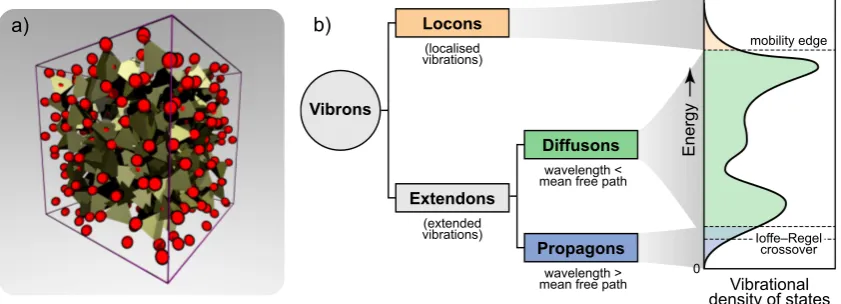
Figure 1. a) A 512-atom structural model of amorphous silicon (a-Si), taken from Ref. 19. The tetrahedrality of the network of silicon atoms (red spheres) is highlighted via the coordination polyhedra. b) Taxonomy of vibrations in glasses and their contributions to the vibrational density of states (VDOS; this sketch is based on Ref. [14]), illustrated for the prototypical case ofa-Si.

quantised lattice vibrational modes, so-called phonons [10, 11]. In amorphous systems, the absence of long-range order leads to a coexistence of localised vibrations and propagating, plane wave-like modes. This poses a significant challenge for molecular simulations, as large structural models (typically containing between one thousand and a million atoms) are needed to avoid imposing an artificial length scale on the structural and vibrational properties of the system [12, 13]. In fact, any atomistic simulation of amorphous matter must be performed in a simulation box with periodic boundary conditions that does have translational symmetry. In addition, we shall see that different computational techniques may be necessary to investigate, say, the different mechanisms of heat conduction in complex disordered systems.

According to the labelling introduced by Allen and Feldman (AF) [14], the entirety of vibra-tional modes (“vibrons”) in amorphous solids consist of localised and extended vibrations (“locons” and “extendons”, respectively). The latter can be further labelled as “propagons” or “diffusons” according to whether or not their wavenumber ω is lower (propagons) or higher (diffusons) than the so-called Ioffe-Regel crossover frequencyωco, for which their mean-free path is comparable to

the wavelength [15]. This is illustrated in Fig. 1 for the prototypical example of amorphous silicon (a-Si). a-Si can be considered as a relatively “simple” amorphous solid, in that its structure can be approximated solely in terms of tetrahedral units (Fig. 1a) [16]. And yet, even this prototypical amorphous solid shows a complex vibrational landscape. Figure 1b illustrates how the a-Si vibra-tional density of states (VDOS) originates from contributions by different types of vibrons. It is also worth noting that the AF framework applies to (quasi)harmonic solids, thus neglecting the contribution of non-harmonic motions, usually described by two-level states (TLS) [17, 18]. While the latter usually play very little role in determining, e.g., the thermal conductivity at room tem-perature, their mention should help to emphasise the sheer complexity of the vibrational landscape of disordered systems (as compared to crystals).

this exciting class of materials below. Clearly, there is a need to better understand the vibrational and thermal properties in nanostructures and nanoconfined environments.

Molecular simulations offer a unique opportunity to obtain microscopic insight into the origin of thermal properties—including disordered systems. This is of clear technological interest: there are ways to alter, say, the thermal conductivity of a given solid, by tuning the extent of disorder (via doping, or intercalation, or nanostructuring) [32]. Computational investigations can thus con-tribute to connect the molecular-level details of materials with macroscopic functional properties, complementing and guiding experiments and applications.

In principle, ab initio simulations (typically based on Density Functional Theory, DFT [33]) would be the tool of the trade to compute properties such as the electronic contribution to the thermal conductivity or, as we shall see in Sec. 3.2, the thermal boundary resistance at interfaces. Unfortunately, the computational requirements to compute properties such as the thermal conduc-tivity are often well beyond the reach ofab initiocalculations. For instance, estimating the thermal conductivity for the phase-change material GeTe (Sec. 3.1.1) required a 4096-atom model and a molecular-dynamics (MD) simulation on a nanosecond timescale. This MD run involved millions of individual time steps, at each of which the forces on atoms need to be evaluated [34]—it be-comes immediately clear why this is not feasible with DFT, which requires very significant effort to converge the wave function of even one single 4096-atom snapshot. Thus, one is typically forced to resort to classical MD, which however poses yet another major issue: that of the availability and accuracy of parametrised force fields. For simple systems, fairly accurate force fields are typically available [35–40]. The same holds for a number of covalent glasses such as silica, for which a number of viable options do exist [41–43]; furthermore, empirical potentials can be significantly improved by physically and chemically motivated modifications, such as environment-dependent cutoff radii [44]. However, the situation is dramatically different when dealing with more complex materials: multicomponent alloys, Li-ion conducting glasses, and chalcogenide glasses for electronic applica-tions are all typically characterised by diverse local atomic environments and varying degrees of disorder—including extended structural defects. Crafting accurate interatomic potentials for such systems is a formidable challenge, one that has been worrying materials scientists for decades.

One way to harness the computational efficiency of classical MD while retaining a good deal of the accuracy of ab initio simulations is to take advantage of machine learning (ML). These are exciting times for the ML community, as these algorithms are quickly spreading through an impressive number of disciplines and technologies [45–48]. In the context of molecular simulations, ML algorithms are used as particularly clever fitting tools to obtain interatomic potentials, starting from data sets of configurations and (typically) energies computedab initio [49]. We shall see that this opens a wealth of possibilities, including an unprecedented opportunity to study thermal properties of complex amorphous solids by means of molecular simulations.

In this Review, we highlight emerging applications of ML-based interatomic potentials (MLIPs) to investigate vibrational and thermal properties of amorphous solids. In particular, we focus on the prototypical phase-change material GeTe, which is of relevance for non-volatile memory applications. We shall see that MLIPs allow not only to compute properties such as thermal conductivity and thermal boundary resistance, but also to cross-validate results from different computational techniques. We also take a quick survey of amorphous carbon, a structurally quite surprisingly complex system for which an MLIP has recently been made. We discuss the need for these sort of potentials, their limitations, and their unique importance in helping us understanding the microscopic subtleties that rule thermal transport in disordered systems. It is worth noting at this stage that ML algorithms have also been used to predict the thermal properties of materials based on large experimental datasets[50, 51]. This is a fascinating topic but has little in common with the construction of interatomic potentials—as such, it will not be covered in this work.

devoted to unravelling, by means of an NNP, the thermal properties of the phase-change material GeTe. Particular emphasis will be on the thermal conductivity and the thermal boundary resistance. In Sec. 4, we present recent work based on a GAP for amorphous carbon and explore future directions. In the Conclusions, we argue that MLIPs can constitute the way forward to tackle molecular simulations of thermal properties of complex amorphous solids. We also address the limitations of MLIPs when it comes to dealing with high levels of material complexity.

2. Machine Learning for Atomistic Simulations: Why and How

The thermal properties of amorphous solids are an excellent example of the challenges for molecular simulations. In this case, accuracy is crucial just as much as computational efficiency: the former, to treat the subtleties of the vibrational landscape; the latter, to enable simulations on large length/long time scales (nm and ns respectively). Accuracy is usually associated with first-principles (ab initio) calculations, computational efficiency with classical molecular dynamics. The question, now, is how to get the best of both worlds? ML-based methods offer a solution, and as such they have been attracting ever-growing interest over recent years [52–62].

Let us start with a word of caution. “Machine learning” as such is doubtlessly a trending concept, far beyond fundamental research: these days, the general public is perfectly aware, if not of what ML is exactly, surely of what we use it for. Pattern recognition is a popular example [63], together with data analysis [64–66], web search engines and personal assistants, not to mention the cele-brated victory of AlphaGo against a human player [67]. However, for the purpose of constructing interatomic potentials, ML algorithms are little more or little less than fairly clever fitting tools. A more detailed review discussing MLIPs can be found, e.g., in Ref. [49]; we here limit ourselves to the basic principles.

MLIPs perform a high-dimensional fit to a given potential-energy surface (PES), and therefore the starting point is to build a database containing roughly 102–104 small configurations (each containing maybe a hundred atoms or molecules), for which it is feasible to compute energies and forces ab initio. Once this database has been created, the connection between atomic structure and potential energy has to be encoded in a suitable form to be fed into the ML algorithm. This requires so-calleddescriptors, mathematical objects that obey certain requisites and represent the local atomic environments (LAEs): imagine sitting on a particular atom and trying to describe everything you see up to a certain cutoff radius (but no further). Once the descriptors have been settled, the ML algorithm feeds upon the information in the database and interpolates, for any arbitrary LAE, its contribution to the potential energy of the system. At this stage, one can hence calculate energies (and, importantly, forces) for any number of LAEs—that is, one can treat even very large systems with trivially linear scaling behaviour.

2.1. Implementations: Neural-Network Potentials and Gaussian Approximation Potentials

A growing number of algorithmic frameworks exist to construct MLIPs; the interested reader is referred to a detailed overview given by Behler [49] as well as several very recent examples that are beyond the scope of this work [68–70]. Here, we shall only consider two arguably successfully used approaches that we have employed in our own research: namely, artificial neural-network potentials as well as Gaussian Approximation Potentials. We do not aim to recommend one over the other—both are useful, and different, approaches towards a similar problem.

NNPs take advantage of feed-forward neural networks to construct a PES starting from the energies of the configurations in the reference database. They provide an analytic representation of the PES, so that computing the forces acting on each atom in the system (which is the basis of MD simulations) is simply a matter of taking the derivative with respect to the atomic positions. The central approximation of NNPs is that the total energyE of a system can be decomposed into a sum of individual contributionsεi,

Etotal =

X

i

εi, (1)

where each of these atomic energies is a function of the LAE of the i-th atom, and the latter is in turn defined using a set of descriptors. NNPs typically employ combinations of so-called Atom-centred Symmetry Functions (ACSFs) for this task [71]: these functions take into account the distances and angles between pairs and triplets of atoms, respectively, and their combination results in a multi-body description of an LAE.

Note that the above expression assumeslocality (“short-sightedness”); that is, it assumes that the energetics and forces of a given atom dependonlyon its immediate environment as specified by a cutoff radius. The latter typically encompasses the first and second coordination shells, leading to cutoff radii of the order of 5-10 ˚A. This approximation applies to NNPs as well, and it is valid for many covalently bonded and metallic materials, while it faces challenges when long-range (ionic and/or dispersion) interactions are present. The latter can implicitly be taken into account by producing a data set with dispersion-corrected/included exchange-correlation functionals. The assumption is that the contributions of such long-range forces lead structural modifications of the systems which can be described within the framework of LAEs - which may or may not be an accurate assumption. In some cases, even a “standard” DFT methodology may lead to a reasonable description: for example, the Local Density Approximation (LDA) functional gives an acceptable value for the inter-layer distance in graphite (one of the reasons it was chosen for the carbon potential described below), whereas standard GGA functionals will fail at this task [72, 73]. Care must be taken in choosing the underlying computational method, as always. The situation is much more complex when dealing with charged systems, where electrostatic interactions play a central role. In that case, charges have to be taken into account. In the case of NNPs, this is done by introducing a dedicated set of neural networks dealing exclusively with the electrostatics. This approach has been successful in e.g. obtaining a NNP for zinc oxide [74].

In the GAP framework, the total energy is likewise decomposed into a sum of individual con-tributions εi, dependent on the LAE of the central atom. In this case, the LAE is encoded by a

so-called “descriptor vector”, which we denote by~qi. The choice of these vectors is arbitrary in the

(possibly) unknown basis functions{φt}, combined using linear combination coefficients,αt.

εi(~qi) =

X

t

αtφt(~qi)≡εi(α, ~~ qi) (2)

These coefficients are determined during the construction of the potential, by fitting to a large database of DFT “training” points (index t), and afterwards kept fixed and tabulated. If we now assume that theαtare normally distributed, we can determine the so-calledcovarianceof two local

energies, comparing an LAE from the training data to a new one, and so finding the energywithout specifically knowing the basis functions themselves. All that is needed to know is an expression for the covariance, also called akernel.

In practice, only a small number of representative, so-called “sparse”, points are selected from the entire training database. This choice can be made at random, or by using advanced tools such as CUR decomposition [76], which ensures that the selected points are distinct from one another to the greatest degree possible. In the case of NNP, the vast majority of the structures contained in the training database is usually taken into account. While a number of technicalities can be used to e.g. avoid/include unnecessary/representative regions of the configurational space, the sparsity of the data set does not play a key role in NNPs—as opposed to the GAP framework.

The idea of using neural networks to fit a PES dates back to the 1990s (see e.g. Ref. 55), whereas a framework capable of dealing with a high-dimensional PES (say, a disordered solid, rather than a single molecule in the gas phase) was introduced in 2007 by Behler and Parrinello [77]. Since then, NNPs have been created for a diverse range of systems, from metal surfaces [78] to water [79].

The GAP framework was introduced in 2010 by Bart´oket al., and interatomic potentials for the bulk phases of carbon, silicon, and germanium were presented at that time, as well as initial proofs-of-concept for GaAs and iron [80]. Subsequently, Szlachta et al. showed how training databases for GAPs can be constructed in a systematic fashion [81], and this has been the paradigm in MLIP development until today. In that case, fitting a GAP model for tungsten, they started with bulk unit cells and then introduced supercell expansions, point defects, surfaces, and dislocations: indeed, the model can “learn” by incorporating additional data [81]. A GAP specifically targeted at an amorphous system was introduced very recently [82], and we will describe this in detail below (Sec. 4). The GAP code is freely available for non-commercial research at http://www.libatoms.org. It consists of two parts: a “prediction” code, which takes parametrised GAP files and uses them to drive simulations (this can be run as a stand-alone program, or via an interface to LAMMPS [83]), and the “training” code which generates a new GAP model from a given set of reference data and input parameters.

It is worth noting that expanding an existing MLIP (for example, from the bulk to surfaces) is usually a one-time investment: once the new DFT reference data have been generated, the potential can be run in a largely similar fashion, and—in the case of GAP—maybe doubles the number of sparse points (with which the speed of the potential scales). A higher price in terms of additional configurations has usually to be paid when extending an NNP to incorporate, e.g. a new phase of the system. Let us say it clearly: MLIPs are fitting tools. They can interpolate the PES, using the information contained in the reference data set, but they cannot extrapolate to regions of configurational space far outside the database. For example, an MLIP needs to have “seen” surfaces, not just bulk phases, to enable accurate predictions of surface energies [81]. This is often an acceptable price to pay for the largely increased flexibility of the resulting MLIPs.

an NNP for molecular solids was proposed, giving access to a wide range of different materials built from organic molecules (containing carbon, hydrogen, oxygen, and nitrogen) [85].

2.2. What are the Limits?

ML-based Interatomic Potentials enable large-scale molecular simulations with quasi-ab initio accu-racy. This outstanding capability comes at a price, though; namely, the sheer computational effort that is usually needed to build (and to expand) the reference data set. As an example, an NNP recently used to investigate the crystallisation kinetics of GeTe nanowires is based on a dataset of about 45,000 configurations—that is, 45,000 DFT calculations were performed to obtain a reliable NNP [86]. This is perhaps an extreme scenario, in that the above-mentioned NNP can deal with bulk phases as well as surfaces and nanostructures—requiring a huge number of configurations to sample the vast configuration space. However, it is safe to say that the most time-consuming part in the creation of an MLIP is the creation of the data set.

Furthermore, a number of technical issues arise with the fitting procedure itself. As a rule, the more complex the system (that is, the more diverse and extended the LAE), the more these issues become important. However, we shall see in Sec. 4 that even a supposedly simple disordered system, such as amorphous carbon, can display a diverse variety of structural features, which lead in turn to a complex interplay between the contribution of the different vibrons (e.g., propagons and diffusons, see Fig. 1b) to the thermal properties of the material. Here follows a non-comprehensive list of the limitations of MLIPs to date:

• Extrapolation: As discussed in Sec. 2.1, MLIPs cannot extrapolate the PES for regions of configurational space that are not represented in the dataset at all.

• Sparse data sets: numerically speaking, it is not easy to produce a MLIP starting from a very sparse data set, i.e. a data set containing configurations, say bulk cells next to surfaces, whose structures and energies differ wildly. This calls for special measures to be put in place, and is the subject of much of the ongoing research aimed at improving MLIPs.

• Long-range interactions: As discussed in Sec. 2.1, taking into account, e.g., dispersion inter-actions requires special care.

• Chemical complexity: Multicomponent systems, such as ternary or even higher alloys and compounds, are difficult to describe with MLIPs. This is because the number of LAEs in-creases with the number of components (and drastically so with each added species), and the increasing difficulty to map a specific LAE onto its energy.

• The accuracy of the underlying reference data: MLIPs are normally fitted to DFT energies and forces, aiming to reproduce them as closely as possible, and often tacitly assuming that the reference data are correct. There are, however, several instances where simple density-functional approximations fail [87–89], and then likewise the MLIP must fail—observingbetter agreement with experiment than the DFT result will be merely a fortuitous coincidence. In the future, we expect that this can be partially alleviated by fitting to higher-level DFT or even wavefunction-based data, as already exemplified for water at the CCSD(T) level [84].

In light of these limitations, it is thus our (very personal) opinion that the construction of a MLIP should only be pursued if:

(1) No other options are available. In many cases, empirical force fields do allow fairly reliable calculations of thermal properties, and nowadays ab initio MD can deal with up to 500 particles for up to 1–2 ns;

elemental solids, and building an MLIP for the whole phase diagram of a molecular system (such as water) can require several years. A scenario where the construction of MLIPs did pay off is that of the phase-change material GeTe, which will be discussed in the next section.

3. Thermal properties of Phase-Change Materials

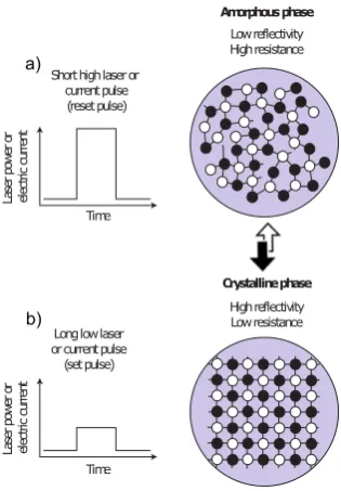
The term “phase-change material” (PCM) can, annoyingly enough, refer to two entirely different classes of systems and applications: PCMs for energy storage (compounds with a high enthalpy of fusion, used to store energy as latent heat) [90, 91], and PCMs for data storage [92–94]. The latter, and only the latter, are the topic of this review. They are typically chalcogenide alloys, with compositions along the quasi-binary tie-line that connects the two binary prototype systems GeTe and Sb2Te3. The amorphous and crystalline phases of these compounds display a sharp contrast in terms of both optical reflectivity and electrical resistance, and can thus be used to store binary bits of information, zeroes and ones, as structural states of the material. Moreover, the phase transition between the amorphous and crystalline phases (and vice versa) takes place in a matter of nanoseconds, and it is perfectly reversible up to millions of cycles. As such, PCMs are widely considered as very promising candidates for the next generation of non-volatile memories. Excellent review articles about PCMs in general can be found, e.g., in Refs. [28–30]; their computational treatment has been discussed in Refs. [95] and [96].

The thermal properties of these systems are of key importance for devices. As illustrated in Fig. 2, both theresetandsetprocesses (writing zeroes and ones, respectively) are induced by heating, using laser pulses in optical media, and voltage-induced Joule heating in electronic memories. In addition, thermal cross-talk between different regions is detrimental for device performance (and limits data density); it is strongly dependent on the thermal conductivity (κ) of both the crystalline and the amorphous phases. A low thermal conductivity is thus desirable, not only to avoid such cross-talk but also to minimise the electrical current needed to induce thereset and setprocesses [30].

Luckily enough, the overwhelming majority of PCMs shows very low thermal conductivity (typ-ically, κ < 1 Wm−1K−1), both in the amorphous and crystalline phases [97, 98]. The low value of κ in Ge–Sb–Te crystals is due to strong phonon scattering from randomly distributed point defects [99, 100]. For instance, in GeTe, the variable concentration of Ge vacancies is responsible for the large spread of the experimental data reported for its bulk thermal conductivity [100].

Concerning the amorphous phases, it is crucial to determine whether propagating vibrons char-acterised by long mean-free paths exist—and to what extent. Thesepropagons substantially con-tribute to the thermal conductivity of, say, amorphous silicon [101], and they are usually absent in nano-structures—simply because their mean-free path is larger than the dimensionality of the system [102]. As phase-change memories rely on active volumes of the material of the order of a few nanometers only, it is thus important to determine whether the values of κ measured for bulk amorphous GeTe can indeed be used to model the thermal properties of this compound in nano-scaled devices.

Despite its seemingly simple chemical composition, amorphous GeTe displays an intriguing co-existence of tetrahedral and defective octahedral LAO [103–105] (illustrated in Fig. 3c), extended defects such as chains of homopolar Ge-Ge bonds [106], and nano-voids [107, 108]; all of these introduce significant challenges for materials modelling and normally requires a description at the ab initio level. While the vibrational properties of this system can be indeed described by ab ini-tiosimulations in small structural models (up to∼500 atoms) [104, 109], a reliable description of macroscopicthermalproperties requires much larger systems (containing 103_-104_{atoms) and longer} simulation times (fractions of ns). This is necessary to take into account the above-mentioned dis-order and diversity in local environments, and to enable thermal-conductivity calculations both by equilibrium and non-equilibrium MD—as we shall see in the next sections.

Time Time Short high laser or

current pulse (reset pulse) La se r p ow er o r el ec tri c cu rre nt La se r p ow er o r el ec tri c cu rre nt Low reflectivity High resistance

Long low laser or current pulse (set pulse) Amorphous phase Crystalline phase High reflectivity Low resistance a) b)

Figure 2. The processes of a)resetand b)setupon which phase change memories are based. In both cases, the active material is heated by either laser or current pulses above its melting temperature. The rapid (≥109 _Ks−1_{) cooling of such a melt leads}

to the amorphous phase illustrated in a). Longer (and less intense) pulses allow for the amorphous phase to crystallise, as depicted in b). Adapted from Ref. [30].

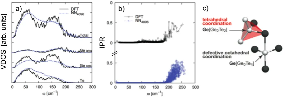
e.g., Refs. [110–113]). In terms of simulations, calculations of κ for a few crystalline phases can be found in the recent literature [100, 114]. Concerning the amorphous phases, however, the only comprehensive study to date is about GeTe, chiefly because a MLIP for this compound has been constructed in 2012 [115]. This MLIP belongs to the family of NNPs, and takes advantage of the approach of Behler and Parrinello [77]. Originally developed for the bulk phases (liquid, crystalline, amorphous) of GeTe, the potential has been recently extended to take into account free surfaces and nano-structures [86]. It allows to perform massively parallel MD simulations: good scaling up to 512 cores can be achieved for systems containing∼104 atoms, which in turn can be simulated for as long as several nanoseconds. A number of applications enabled by this potential have been reported, addressing crystallisation kinetics [116] or dynamical properties of the supercooled liquid [106, 117], for example. This NNP has been extensively validated in terms of structural and, most importantly here, vibrational properties compared with DFT calculations [115]. Figure 3a compares the VDOS for a 4096-atom model of amorphous GeTe with DFT data for a much smaller (216-atom) model. The agreement is remarkable, especially considered that the different contributions to the total VDOS originating from the different LAO are correctly captured by the NNP. The same holds for the Inverse Participation Ratio (IPR; Fig. 3b), which quantifies the degree of localisation of each vibron, and is defined as

IPRj = PN i=1 ¯

e_√(j,i)

mi 4 PN i=1

|¯e(j,i)|2 mi

2, (3)

where ¯e(i, j) is thej-th vibron eigenvector for thei-th atom with mass mi. The value of this IPR

a) b) c)

V

DOS

[ar

b.

un

its]

IPR

Figure 3. a) VDOS of a 4096-atom model of amorphous GeTe; both the structure and the vibrational properties were obtained using an NNP. The projections of the total VDOS on different atomic species (Getetra/octa refer to Ge atoms sitting in tetrahedral and defective octahedral LAEs, see panel c) is also reported. The results are compared with those obtained for a smaller (216-atom) model via DFT calculations. b) Inverse participation ratio (IPR, see text) of phonons (orvibrons) in amorphous GeTe. Adapted from Ref. [118]. c) Coexistence of tetrahedral and defective-octahedral coordination motifs in GeTe. Adapted from Ref. [105].

3.1. The Thermal Conductivity of Amorphous GeTe: Three Options

Experimental values for the thermal conductivity (κ)ofa-GeTe range from 0.2 to 0.4 Wm−1K−1[97, 119, 120]. As for the simulations, we have different options: equilibrium molecular-dynamics (EMD), non-equilibrium molecular-dynamics (NEMD), and the analysis of both diffusons and propagons by means of AF theory and the Boltzmann Transport Equation (BTE), respectively. The computa-tional efficiency of MLIPs has now allowed us to compare theκvalues calculated by these different approaches side-by-side. This is a unique opportunity to strengthen the reliability of molecular simulations in investigating thermal properties of amorphous solids. In the following sections, we shall consider each of the three above-mentioned computational options.

The total thermal conductivity in a system is given by

κ=κLattice+κElectronic, (4)

where the lattice thermal conductivity originates from vibrons (both in insulating and metallic systems), and the electronic thermal conductivity is due to free conduction electrons (thus relevant for metallic systems only). Amorphous GeTe displays a pseudo-gap in the electronic density of states [121], and as such the contribution of κElectronic can reasonably be considered as being negligible. In fact, the calculations ofκwe are about to discuss refer toκLatticeonly—and we shall see that those account for the whole value of the totalκ, confirming the above assumption. It is also worth noticing thatκ in principle is a tensorial quantity. This is especially relevant for crystalline systems: for instance, in the well-ordered crystalline phase of Ge2Sb2Te5, weak Te–Te bonds along the hexagonalc-axis lead to a strongly anisotropic thermal conductivity [100].

3.1.1. Green–Kubo Relation

Transport coefficients, such asκ, can be computed via the so-called Green–Kubo relation from the integrals of specific time-correlation functions. For the thermal conductivity [122],

κ= 1

3kBT2Ω

3

X

α=1

Z ∞

0

Ω, α, and Jα(t0) stand for the volume of the simulation box, the α-th Cartesian coordinate and

the energy flux, respectively. The latter is also known as the heat flux or the (microscopic) heat current, and it can in turn be written as [122]

Jα(t0) = N X

i=1

i(t0)·vi,α(t0)−

N X

i=1 3

X

β=1

σi,αβ(t0)·vi,β(t0), (6)

wherei(t0),vi,α(t0) andσi,αβ are the total energy of thei-th atom, its velocity at timet0, and the

element of the atomic stress tensor, respectively. The first term in Eq. 6 is commonly referred to as aconvective term, as it accounts for the heat current originating from atomic motion (convection). It is the main contribution to Jα(t0) in gases, important in liquids, but basically negligible for

solids, where the self-diffusion is exceedingly low. We thus consider exclusively the second term in Eq. 6, which originates from interatomic interactions and it is associated with heat conduction; it is commonly labelled as thevirial term.

Note that partitioning the total stress into single-particle contributions depends on the particular form of the interatomic potential [123]; in some cases, more than one choice is available. However, in the framework of Behler–Parrinello NNPs, the total energy of the system is written as a sum of individual atomic energies, so that the definition of an atomic stress follows in a straightforward manner. Note, also, that Green-Kubo relations can be used inanyequilibrium ensemble, albeit the specific form of Jα(t0) is different within different ensembles [122]. Eq. 6 refers to the canonical

ensemble (“NVT”).

The time-correlation function in Eq. 5 can be obtained by EMD. This is straightforward in principle, and yet substantial statistics are needed to address the tails of the correlation function of the energy flux—and thus to converge the integral in Eq. 5. One way to improve numerical accuracy and achieve faster convergence is to rewrite Eq. 5 by taking advantage of the Einstein relation [124]:

κ = _6k 1

BT2Ωlimt→∞ d dt

PN i=1

P3

α=1h[ζi,α(t)−ζi,α(0)]2i, with (7)

ζi,α(t)−ζi,α(0) = Rt

0Ji,αdt

0 ₍₈₎

In the case ofa-GeTe, the truncation time tin the integral above was set to 40 ps (Fig. 4a), and yet 2 ns-long (corresponding in this case to 1,000,000 time steps) simulations were necessary to accumulate sufficient statistics to obtain the value of κ reported in Fig. 4d, which is converged within 0.05 Wm−1K−1. A number of different methods, such as Homogeneous Non-Equilibrium MD, have been recently proposed to overcome the numerical challenges imposed by the original Green–Kubo approach [127].

3.1.2. Non-Equilibrium Molecular Dynamics

law [129]:

κ=− qα

dT /dα, (9)

where qα is the (imposed) heat flux along the α direction. The value of κ fora-GeTe from these

NEMD simulations is 0.26±0.05 Wm−1K−1 [130], in excellent agreement with the outcome of EMD simulations using the Green–Kubo formula (0.27±0.05 Wm−1K−1) [118].

3.1.3. Allen–Feldman Theory and the Boltzmann Transport Equation

The equilibrium (Green–Kubo) and non-equilibrium (M¨uller–Plathe) MD methods described above take into account all the vibrations of the system: they do not distinguish, say, between localised or extended phonons. As discussed in Sec. 1, however, different types of phonons contribute to different extents to the vibrational density of states, and thus, to the thermal conductivity. It would thus be desirable to understand which phonons are responsible for the total value of κ. Recalling the taxonomy illustrated in Fig. 1, we have:

κTotal=κLocons+κPropagons+κDiffusons. (10)

In the case of GeTe, we have not taken into account localised modes (locons). Although such vibrations do populate the high-frequency tail of the VDOS (see Fig. 2), their contribution to

κTotal is negligible, as will be discussed below. κPropagons can be obtained by solving the linearised Boltzmann transport equation (BTE) in the single-mode relaxation-time approximation [131]:

κPropagons=κBTE= 1 3

N X

j=1

cj·v2g,j·τj, (11)

wherecj,vg,j andτjare the specific heat per unit volume, the group velocity, and the lifetime of the

(harmonic)j-th phonon calculated at the supercell Γ point, respectively. Whilecj andvg,j can be

straightforwardly calculated from the dispersion curvesωj(q) (see, e.g., Ref. [118]), the estimation

of the phonon lifetimesτj typically requires to converge the following auto-correlation function:

τj = 2·

Z ∞

0

hEj(t)Ej(0)i

hEj(0)Ej(0)i

, (12)

where Ej(t) = _N1|PNi=1 √

Mie¯j, i·v¯i(t)|2 is the kinetic energy of the j-th mode. Similarly to the

auto-correlation function described in Eq. 5 in the case of the Green–Kubo approach, long (2 ns) MD trajectories were needed to converge the values ofτj for a-GeTe, once more highlighting the

need for efficient yet accurate MLIPs. It is also worth noticing that, in the case of GeTe, the single-mode relaxation-time approximation of the BTE appears to be valid. In fact, the energy of the phonons does decay following a single exponential relaxation behaviour (Fig. 3c). Other options to estimate the lifetimesτj have been proposed, albeit most of the formulations have been validated

for crystalline systems only [132–134].

Perhaps surprisingly, in a-GeTe the overwhelming majority of vibrational modes show a very short mean free path (λj = vg,j ·τj), no longer than 10 ˚A [118]. This is radically different from

what has been observed, e.g. in a-Si, where values of λj up to 102 ˚A have been reported [101].

In fact, κDiffusons accounts for most of the total thermal conductivity in a-GeTe. Within the theory of Allen and Feldman, eachj-th vibron has a diffusivity[14, 135]:

Dα,j =

Ω2 8π2_~2_ν2

i X

n6=j

|h¯ej|Jα|¯eni|2δ(νj −νn), (13)

whereh¯ej|Jα|¯eni are the matrix elements of the α Cartesian component of the energy-flux

op-erator (Eq. 6) between two (harmonic) normal modes ¯ej and ¯en, with frequencies νj and νn,

respectively. The resulting contribution to the thermal conductivity is frequency-dependent, and it can be written as [14, 135]

κDiffusons =κAF =

N X

j=1

cj

1 3

3

X

α=1

Dα,j. (14)

As seen in Fig. 3d, κDiffusons is indeed the major contributor to the thermal conductivity of a-GeTe. This behaviour is in stark contrast with what has been observed, e.g., for a-Si, where propagons also play an important role and indeedκTotal ≈ 1₂κPropagons+ 1₂κDiffusons [101]. A per-haps simplistic explanation is that a-Si is, compared to a-GeTe, a rather homogeneous system characterised by a relatively low degree of disorder [19, 136–138], so that propagons can actually extend over very long mean-free paths. In contrast, the structure ofa-GeTe includes very different local atomic environments as well as nano-cavities and extended defects [103, 139]. These structural features scatter and hinder the spatial extent of the propagons, which in turn lead to exceedingly low values of κBTE fora-GeTe.

At this point, we hope that the reader would be convinced that molecular simulations of vibra-tional and thermal proprieties of amorphous solids need to address a number of different, often non-trivial aspects. Assessing which type of vibrons contribute to the thermal conductivity is a good example, as such insight allows to guide experiments and applications. For instance, in a -GeTe, the absence of spatially extended propagons suggests that the value ofκ measured for bulk samples can be safely used to model thermal conductivity at the nanoscale as well—this is of great practical importance for assessing the device performance. On the other hand, the substantial con-tribution of propagons in a-Si presents the opportunity to tune the thermal conductivity of the material by nanostructuring.

3.2. Thermal Boundary Resistance at the Crystal–Amorphous Interface

We have discussed in Sec. 3 the importance of the thermal conductivity for PCM used for non-volatile memories. The latter ultimately rely on the crystallisation/amorphisation of materials such as GeTe, so that the thermal boundary resistance (TBR) between the crystal and the amorphous phase plays a crucial role for device performance. In fact, it is worth investigating the TBR not only at the crystal/amorphous interface, but also at the interfaces between the PCM and the other components of the actual memory cell (dielectrics, such as silicon oxide or silicon nitride, as well as electrode metals such as TiN and Al). In some cases,ab initiosimulations can be used to study the TBR at the interface between different crystalline phases [100]. However, computing the TBR between the amorphous phase and the crystal does, once more, require the help of MLIPs.

0 0.05 0.1 0.15 0.2 0.25 0.3 0.35

0 50 100 150 200 250

κ

[W/

mK]

ω [cm−1]

BTE AF+BTE EMD NEMD

d)

a)

0 5 10 15 20 25 30 35 40

< J

x

(0) J

x

(t)> / < J

x (0) J x (0)> Time [ps] 0 2 4 6 8 10 12 14 16

0 5 10 15 20 25 30 35 40

JMSD [J 2m 2] Time [ps] MSD linear fit

re 4.1: Normalized autocorrelation function of the energy current operator. Inset s the MSD of J according to Eq. 4.5.

value ofκ is close to those measured experimentally for GexTe1−x and GeSbTe

1], all in the range 0.1-0.3 W/mK, including Ge0.20Te0.80 (0.19 W/mK) [12]. An

ental value of κ is available also for a-GeTe [129] which, however, is about 2.5 ), one order of magnitude larger than our result and than other experimental data similar systems. The origin of this discrepancy is unclear and suggests the need of erimental measurements on a-GeTe.

value ofκobtained by MD simulations (either via the Green-Kubo approach or the irect method) accounts for the whole value of the lattice thermal conductivity, that lects all contributions coming from the vibrational modes of the systems. However, ssed in section 1.3 in the case of amorphous materials, there exist different kind ns, each one contributing to the total value ofκ by a different mechanism. It is e important to investigate further the microscopic origin ofκto identify which and

extent different phonons contribute to thermal conductivity.

0

0.1

0.2

0.3

0.4

0.5

0.6

0.7

0.8

0.9

1

0

5

10

15

20

25

30

35

40

Time [ps]

0 5 10 15 20 25 30 35 40

JMSD [J 2m 2] Time [ps] MSD linear fit

alized autocorrelation function of the energy current operator. Inset J according to Eq. 4.5.

close to those measured experimentally for Ge

Te

and GeSbTe

range 0.1-0.3 W/mK, including Ge

Te

(0.19 W/mK) [12]. An

f

κ

is available also for a-GeTe [129] which, however, is about 2.5

of magnitude larger than our result and than other experimental data

ms. The origin of this discrepancy is unclear and suggests the need of

asurements on a-GeTe.

200 250 300 350 400

0 1 2 3 4 5 6 7 8 9 10

Temperature [K]

L [nm]

b)

sizably to the thermal conductivity of a-GeTe.

−0.1 0 0.1 0.2 0.3 0.4 0.5 0.6 0.7 0.8 0.9 1

0 0.2 0.4 0.6 0.8 1 1.2

En

(t)

Time [ps] Exp. fit

F igure 4.2: Decay of the energy of a normal mode at ∼150 cm− 1_{as a function}

4.2 Diffusons

In section 1.3, we introduced diffusons. They are extended, delocalized and not modes. Thus, their contribution to thermal conductivity cannot be computed anharmonic hopping models. In the early nineties Allen and Feldman propos that specifically takes into account diffusons. The theory applies when disorder to make the majority of states to propagate very little, but insufficient to make a localized. Also it is necessary that the material is stiffenough or the temperature that the harmonic approximation is applicable. In this model, localized state no heat current (anharmonic terms are needed for hopping). Nevertheless, sign currents are carried by diffusons. The basic idea is that the heat current oper diagonal matrix elementsJi j between the harmonic for foamy systems. The st is the Kubo formula of Eq. 4.3. For a disordered harmonic solid the exact many are simply the various ways of occupying the 3N harmonic-oscillator states. I down the heat current operator in terms of these oscillator states [39], it is possi

c)

Figure 4. a) Normalised auto-correlation function of the energy-current operator. The inset shows the MSD ofJ according to Eq. 8. b) Temperature profile in a reverse NEMD simulation of bulka-GeTe. Grey, blue and red shaded regions depict the fixed atoms, the cold source and the hot source, respectively. The continuous dark-blue line represents the linear fit of the data. c) Decay of the energy of a vibron ofa-GeTe at∼150 cm−1 _{as a function of time. d) The thermal conductivity}

κof amorphous GeTe calculated by means of a NNP using three different approaches. Equilibrium MD simulations taking advantage of the Green-Kubo relation (EMD), non-equilibrium MD simulations using the M¨uller-Plathe approach (NEMD), and quasi-static calculations (AF+BTE) addressing the contributions of diffusons (according to the Allen-Feldman formalism, AF) and propagons (taken into account by computing the Boltzmann Transport Equation, BTE). In the case of AF+BTE, the reported value of the thermal conductivity for a given frequencyω∗has been obtained by summing the contributions of all phonons characterised byω≤ω∗_{. Adapted from Ref. [118].}

orders of magnitude) than that of the amorphous phase [100]. As such, heat is carried by electrons and phonons alike in the crystal, but only by phonons in the amorphous phase. In addition, while in crystalline GeTe the thermal conductivity originates chiefly from propagons (κTotal ≈κBTE) [100], we have seen in Sec. 3.1.3 that ina-GeTeκTotal ≈κDiffusons ≈κAF. A theoretical approach taking this evidence into account has been developed by Majumdar and Reddy [140], and it is based on the following expression for the TBR:

TBRTotal = TBRLattice+ TBRElectronic, (15)

a)

b)

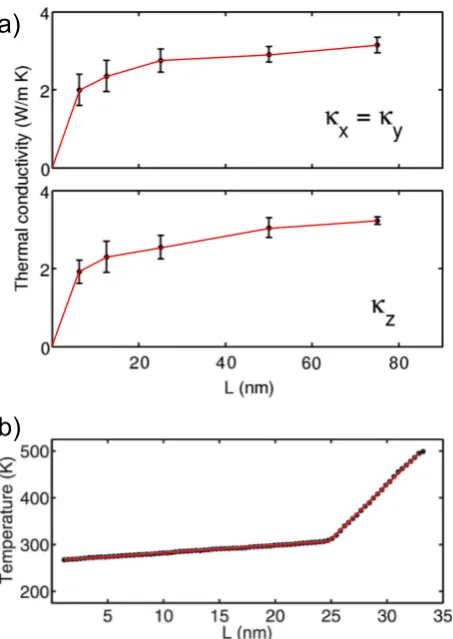
Figure 5. a) Thermal conductivityκof crystalline (trigonal) GeTe as a function of the length of the simulation cellL(along the direction of the heat flux). The contributions toκ, split into perpendicular and parallel (with respect to thec-axis of the trigonal crystal) components, are reported in the upper and lower panels, respectively. b) Temperature profile observed in an NEMD simulation of the junction between amorphous and crystalline GeTe. The amorphous/crystalline interface lies on the (0001) crystalline plane of the trigonal crystal (hexagonal cell setup). Adapted from Ref. [130].

TBRElectronic can be written as [140]

TBRElectronic=

κElectronic

κTotal

3₂

·(κLatticeGe−ph)− 1

2, (16)

where the parameter G depends on the electron-phonon coupling constant λe−ph as well as the

electronic density of states at the Fermi level (see, e.g., Ref. [130] for further details). At this stage, it should be quite clear why we need a mixture ofab initio and classical simulations to deal with TBR: the calculation of the electron-phonon coupling constant lies within the remit of ab initio (DFT) simulations only, whereas large simulation boxes and long simulation times are needed to extract TBRLattice in the framework of, e.g., the NEMD simulations that we have previously discussed.

reported in Fig. 4a. Note that supercells as large as 80 nm were needed to converge the NEMD simulations. The same can be said for the NEMD calculations of the actual TBR, which led to the temperature profile depicted in Fig. 4b: the jump in the temperature profile for L ≈ 25 nm in Fig. 4b corresponds to the location of the junction between the crystalline and the amorphous phases. Interestingly, it turns out that the electronic contribution to the TBR is a function of the concentration of Ge vacancies that occur in the crystalline phase of GeTe [100]. These defects induce the formation of holes in the valence band, thus affecting the electron–phonon coupling constant. On average, though,T BRElectronic at the amorphous/crystalline interface is of the same order of magnitude as theT BRLattice reported for PCMs in contact with metallic systems such as TiN and Al [100].

The substantial body of work on the vibrational and thermal properties ofa-GeTe has been made possible by the construction of a dedicated MLIP. We can only hope that this specific example will foster the creation of new generations of MLIPs in the future, thereby enabling the community to tackle ever more complex disordered systems. To substantiate this point, we will now turn to a different but likewise complex material for which an MLIP has been introduced very recently.

4. From Structural to Vibrational to Thermal Properties in Amorphous Carbon

The large structural diversity in allotropes and compounds of carbon goes back to the element’s abil-ity to form very diverse coordination environments: these are conventionally dubbed “sp” (twofold bonded), “sp2” (threefold bonded), and “sp3” (fourfold bonded) in the community. In amorphous carbon (a-C), the situation is even more challenging, as these fragments readily exist side-by-side. The dense form, so-calleddiamond-like(or tetrahedral) amorphous carbon in fact contains a mix-ture of sp2and sp3environments; at low densities, linear –C≡C– chains become influential. Indeed, sample density is a key determinant for the structures (and thus properties) of amorphous forms of carbon [141]. A recent review, including several computational aspects, is found in Ref. [142].

This large structural diversity makes it very challenging to accurately describea-C in atomistic simulations. While landmark potentials, such as that by Tersoff [143] and Brenner [144], have long been providing useful insight, they may have significant issues such as with the abundance of sp3 configurations or the description of failure processes. Many of these issues have later been remedied, e.g., by using an appropriate environment-dependent cutoff [44], but challenges remain.

Recently, some of us have generated a GAP for liquid and amorphous carbon. In this work, we also introduced an improved set of local descriptors that combines the hitherto employed SOAP with local, two- and three-body terms. This was found to be very useful to stabilise the potential in regions of high interatomic forces: in the liquid phase at 9,000 K, interatomic forces in carbon regularly exceed 10 eV ˚A−1, whereas in amorphous carbon at room temperature, they are on the order of only a few eV ˚A−1.

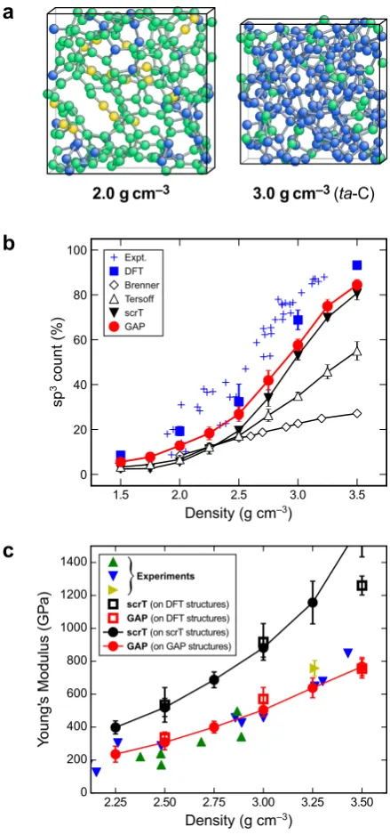
The new a-C GAP [82] has been validated in several ways. Figures 6b–c collect two of the most crucial quality indicators. In the upper panel, we show the sp3 _{count as a function of sample} density. We have further validated the potential by using it for crystal-structure searching, in the spirit of Ref. [145], which led to the identification of several hitherto unknown carbon allotropes [146]. In particular, we fitted a version of the potential that had “seen” no crystalline structures whatsoever—this shows that the PES is trained sufficiently well from liquid and amorphous snap-shots to perform ab initiorandom structure searching (AIRSS)-like procedures [145].

3.0 gcm–3 _(ta-C)

2.0 gcm–3

2.25 2.50 2.75 3.00 3.25 3.50

Density (g cm–3₎

0 200 400 600 800 1000 1200 1400

You

ng

's

M

od

ul

us

(G

Pa

) Experiments

scrT(on DFT structures)

GAP(on DFT structures)

scrT(on scrT structures)

GAP(on GAP structures) Expt.

Brenner Tersoff scrT DFT

GAP

100

80

60

40

20

0

sp

3 count

(%

)

1.5 2.0 2.5 3.0 3.5

Density (g cm–3₎ a

b

c

Figure 6. Modelling amorphous carbon and its key properties by ML-based and other simulation methods. (a) Structural models ofa-C at 2.0 g·cm−3 (left) and ofta-C at 3.0 g·cm−3 (right), generated by quenching from the melt using DFT-MD simulations. In both, the coexistence of sp2 _{and sp}3 _{environments (green and blue, respectively) is apparent; coordination}

numbers have been determined by counting atomic neighbours up to a 1.85 ˚A cutoff. (b) Count of sp3 _{atoms, as defined}

above, as a function of sample density, comparing results from various empirical interatomic potentials, as well as our GAP, to experimental and DFT-based reference data. (c) Same for Young’s modulus: coloured symbols indicate experimental data from various references (cf. Ref. [82]); results from our GAP are compared to those of a state-of-the-art empirical interatomic potential. Adapted with permission from Ref. [82].

0

0.1

0.2

0.3

0.4

0.5

0.6

0.7

0.8

0.9

500 1000 1500 2000

V

DO

S

(A

rb.

unit

s)

ω

[cm

]

2.11 g/cm3_DFT

2.11 g/cm3_GAP

3.37 g/cm3_DFT

3.37 g/cm3_GAP

Diamond_Exp.

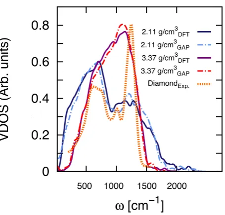
Figure 7. The vibrational density of states (VDOS) of two 216-atom models of amorphous carbon generated as described in Ref. [82] at two different densities: 2.11 and 3.37 g/cm3_{. A comparison between the VDOS computed via GAP (dashed lines)}

and that obtained by DFT-LDA calculations (solid lines) is reported. The experimental VDOS of polycrystalline diamond (DiamondExp.), from Ref. [147]) is also shown – the intensity has been rescaled to the maximum value of the GAP VDOS for

high-density a-C.

low-density (2.11 g/cm3) a-C displays its mean peak at lower frequencies (≈750 cm−1), while the feature corresponding to sp3 carbon is weaker. This is consistent with the fact that low-densitya-C contains a much higher fraction of sp2 (and, if rapidly quenched from the melt, even of close-to-linear sp) atoms, which lead to vibrational modes characterised by lower frequencies compared to that of sp3 carbon. Conversely, the vast majority of atoms in high-density a-C are sp3 hybridized, which lead to a VDOS quite similar to that of polycrystalline diamond.

A full characterisation of the vibrational properties of amorphous carbon at different densities, with special emphasis on the structural features underlying the shape of the VDOS, will be the subject of future work.

5. Conclusions

Our understanding of the thermal properties of amorphous solids has a direct impact on countless practical applications, from optical fibres to digital memories. In principle, molecular simulations could provide valuable insight into the microscopic origin of functional properties, such as thermal conductivity and thermal boundary resistance. However, the absence of long-range order in amor-phous solids requires simulation time and length scales far beyond the reach ofab initiomethods. Conversely, more often than not, simple classical force fields are not able to describe the structural complexity of these amorphous materials.

Machine Learning-based Interatomic Potentials (MLIPs) offer a way to overcome this standoff, as they allow to perform simulations almost as fast as classical MD—while retaining an accuracy typical of first-principles simulations. The field of MLIPs is developing at a fantastic rate: we have briefly reviewed Neural Network Potentials (NNPs) and Gaussian Approximation Potentials (GAPs), but a number of interesting alternatives are emerging as well. Given the huge momentum presently driving the field of machine learning as a whole, it is reasonable to foresee a rapid expansion of MLIPs for molecular simulations in the very near future.

thermal properties of GeTe, a prototype phase-change material for non-volatile data storage. An NNP for this system was built in 2012, and more recently expanded from the crystalline, liquid, and amorphous bulk to free surfaces and low-dimensional nanostructures. This potential allowed to quantify the thermal conductivity of amorphous GeTe, and to pinpoint its microscopic origin. The thermal boundary resistance across the interface between the amorphous and crystalline phases has also been calculated, and it is worth noting that the MLIPs for GeTe allowed for the cross-validation of several results obtained by completely different simulation methods—something exceedingly difficult to achieve by means ofab initiosimulations.

We also explored the capabilities of a GAP recently built to study amorphous carbon, which is widely used in the form of thin films for coatings. This system is especially interesting in that it displays substantial structural differences according to different densities. How does this affect the vibrational and thus the thermal properties? To lay the groundwork for exploring this question, we have here reviewed extensive validation againstab initiosimulations, and presented the results of a preliminary investigation of the vibrational properties as a function of density. The latter suggests that the heat-conduction mechanism in the two phases could be substantially different, and calls for simulations on a much larger scale which are going to be the subject of future work.

The NNP for GeTe and the GAP for amorphous carbon we discussed in here offer unique insight into the thermal properties of these disordered solids. Broadly speaking, we believe that MLIPs provide the opportunity to understand the microscopic origin of functional properties such as thermal conductivity and thermal boundary resistance. This knowledge can aid the design of novel amorphous systems with unique thermal properties, and contribute to bridge the gap between continuous models for thermal transport and molecular simulations. We feel there is enormous potential for the field—even more so as GAP and other frameworks are now publicly available, thus providing the community with the tools of the trade.

The most pressing challenge for MLIPs in the context of thermal properties if perhaps that of addressing the interfaces between different materials, as well as industrially relevant materials such as ceramic matrix composites. The huge configurational space, together with the intrinsic complex-ity of surfaces and interfaces call for further improvements to the existing MLIP implementations. In this respect, we hope that this work will encourage the community to take advantage of the ca-pabilities of MLIPs so as to establish molecular simulations as the method of choice to complement and guide the experimental characterisation of the thermal properties of amorphous solids.

5.1. Acknowledgements

5.2. Disclosure

The authors declare no competing financial interest.

5.3. Funding

G.C.S. is grateful to the Centre for Scientific Computing at the University of Warwick for provid-ing computational resources. V.L.D. gratefully acknowledges a Feodor Lynen fellowship from the Alexander von Humboldt Foundation, a Leverhulme Early Career Fellowship, and support from the Isaac Newton Trust.

References

[2] B. Gotsmann and M. A. Lantz, “Quantized thermal transport across contacts of rough surfaces,”Nat. Mater., vol. 12, p. 3460, Oct. 2012.

[3] M. Beekman, D. T. Morelli, and G. S. Nolas, “Better thermoelectrics through glass-like crystals,”Nat. Mater., vol. 14, pp. 1182–1185, Nov. 2015.

[4] B. Russ, A. Glaudell, J. J. Urban, M. L. Chabinyc, and R. A. Segalman, “Organic thermoelectric materials for energy harvesting and temperature control,”Nat. Rev. Mater., vol. 1, p. 201650, Aug. 2016.

[5] S. Kwon, J. Zheng, M. C. Wingert, S. Cui, and R. Chen, “Unusually High and Anisotropic Thermal Conductivity in Amorphous Silicon Nanostructures,”ACS Nano, vol. 11, pp. 2470–2476, Mar. 2017. [6] A. Shanker, C. Li, G.-H. Kim, D. Gidley, K. P. Pipe, and J. Kim, “High thermal conductivity in

electrostatically engineered amorphous polymers,”Sci. Adv., vol. 3, p. e1700342, July 2017.

[7] M. C. Wingert, J. Zheng, S. Kwon, and R. Chen, “Thermal transport in amorphous materials: a review,”Semicond. Sci. Technol., vol. 31, no. 11, p. 113003, 2016.

[8] D. G. Cahill, P. V. Braun, G. Chen, D. R. Clarke, S. Fan, K. E. Goodson, P. Keblinski, W. P. King, G. D. Mahan, A. Majumdar, H. J. Maris, S. R. Phillpot, E. Pop, and L. Shi, “Nanoscale thermal transport. II,”Appl. Phys. Rev., vol. 1, p. 011305, Jan. 2014.

[9] T. T. Tritt,Thermal conductivity: theory, properties, and applications New York, Springer US, 2004. DOI: 10.1007/b136496.

[10] M. T. Dove, “Introduction to the theory of lattice dynamics,” Journ´ees de la Neutronique, vol. 12, pp. 123–159, 2011.

[11] H. Ibach and H. L¨uth,Solid-State Physics. Berlin, Heidelberg: Springer Berlin Heidelberg, 2009. DOI: 10.1007/978-3-540-93804-0.

[12] D. Sopu, J. Kotakoski, and K. Albe, “Finite-size effects in the phonon density of states of nanostruc-tured germanium: A comparative study of nanoparticles, nanocrystals, nanoglasses, and bulk phases,” Phys. Rev. B, vol. 83, p. 245416, June 2011.

[13] D. Donadio and G. Galli, “Temperature Dependence of the Thermal Conductivity of Thin Silicon Nanowires,”Nano Lett., vol. 10, pp. 847–851, Mar. 2010.

[14] P. B. Allen, J. L. Feldman, J. Fabian, and F. Wooten, “Diffusons, locons and propagons: Character of atomic vibrations in amorphous Si,”Philos. Mag. B, vol. 79, pp. 1715–1731, Nov. 1999.

[15] S. N. Taraskin and S. R. Elliott, “Ioffe–Regel crossover for plane-wave vibrational excitations in vit-reous silica,”Phys. Rev. B, vol. 61, pp. 12031–12037, May 2000.

[16] F. Wooten, K. Winer, and D. Weaire, “Computer Generation of Structural Models of Amorphous Si and Ge,”Phys. Rev. Lett., vol. 54, pp. 1392–1395.

[17] A. W¨urger and D. Bodea, “Thermal conductivity by two-level systems in glasses,” Chem. Phys., vol. 296, pp. 301–306, Jan. 2004.

[18] T. P´erez-Casta˜neda, C. Rodr´ıguez-Tinoco, J. Rodr´ıguez-Viejo, and M. A. Ramos, “Suppression of tunneling two-level systems in ultrastable glasses of indomethacin,”PNAS, vol. 111, pp. 11275–11280, Aug. 2014.

[19] M. J. Cliffe, A. P. Bart´ok, R. N. Kerber, C. P. Grey, G. Cs´anyi, and A. L. Goodwin, “Structural simplicity as a restraint on the structure of amorphous silicon,”Phys. Rev. B, vol. 95, p. 224108, June 2017.

[20] W. Mi-tang and C. Jin-shu, “Viscosity and thermal expansion of rare earth containing soda-lime-silicate glass,”J. Alloys Compd., vol. 504, pp. 273–276, Aug. 2010.

[21] M. L. Baesso, J. Shen, and R. D. Snook, “Time-resolved thermal lens measurement of thermal diffu-sivity of soda-lime glass,”Chem. Phys. Lett., vol. 197, pp. 255–258, Sept. 1992.

[22] M. Oguma, C. J. Fairbanks, and D. P. H. Hasselman, “Thermal Stress Fracture of Brittle Ceramics by Conductive Heat Transfer in a Liquid Metal Quenching Medium,” J. Am. Ceram. Soc., vol. 69, pp. C–87, Apr. 1986.

[23] J. Kang and B. Han, “First-Principles Study on the Thermal Stability of LiNiO2 Materials Coated

by Amorphous Al2O3with Atomic Layer Thickness,”ACS Appl. Mater. Interfaces, vol. 7, pp. 11599–

11603, June 2015.

[24] N. Nitta, F. Wu, J. T. Lee, and G. Yushin, “Li-ion battery materials: present and future,” Mater. Today, vol. 18, pp. 252–264, June 2015.

Materials (A. Tiwari, F. Kuralay, and L. Uzun, eds.), pp. 321–354, John Wiley & Sons, Inc., 2016. DOI: 10.1002/9781119242659.ch8.

[26] S. V. Pershina, A. A. Raskovalov, B. D. Antonov, and O. G. Reznitskikh, “The transport and thermal properties of glassy LiPO3/crystalline Al2O3 (ZrO2) composite electrolytes,” Ionics, pp. 1–6, June

2017.

[27] M.-T. F. Rodrigues, G. Babu, H. Gullapalli, K. Kalaga, F. N. Sayed, K. Kato, J. Joyner, and P. M. Ajayan, “A materials perspective on Li-ion batteries at extreme temperatures,”Nat. Energy, vol. 2, p. 17108, July 2017.

[28] S. Raoux, W. Welnic, and D. Ielmini, “Phase Change Materials and Their Application to Nonvolatile Memories,”Chem. Rev., vol. 110, pp. 240–267, Jan. 2010.

[29] A. V. Kolobov, J. Tominaga (Eds.), Chalcogenides: Metastability and Phase Change Phenomena. Springer, Berlin, Heidelberg 2012.

[30] M. Wuttig and N. Yamada, “Phase-change materials for rewriteable data storage,”Nat. Mater., vol. 6, pp. 824–832, Nov. 2007.

[31] S. Raoux and M. Wuttig,Phase Change Materials: Science and Applications. Springer US, 2010. [32] K. S. Siegert, F. R. L. Lange, E. R. Sittner, H. Volker, C. Schlockermann, T. Siegrist, and M. Wuttig,

“Impact of vacancy ordering on thermal transport in crystalline phase-change materials,”Rep. Prog. Phys., vol. 78, no. 1, p. 013001, 2015.

[33] S. Baroni, S. de Gironcoli, A. Dal Corso, and P. Giannozzi, “Phonons and related crystal properties from density-functional perturbation theory,”Rev. Mod. Phys., vol. 73, pp. 515–562, July 2001. [34] M. E. Tuckerman and G. J. Martyna, “Understanding Modern Molecular Dynamics: Techniques and

Applications,”J. Phys. Chem. B, vol. 104, pp. 159–178, Jan. 2000.

[35] R. N. Barnett, C. L. Cleveland, and U. Landman, “Structure and Dynamics of a Metallic Glass: Molecular-Dynamics Simulations,”Phys. Rev. Lett., vol. 55, pp. 2035–2038, Nov. 1985.

[36] F. Ercolessi, E. Tosatti, and M. Parrinello, “Au (100) Surface Reconstruction,” Phys. Rev. Lett., vol. 57, pp. 719–722, Aug. 1986.

[37] G. J. Ackland and R. Thetford, “An improved N-body semi-empirical model for body-centred cubic transition metals,”Philos. Mag. A, vol. 56, pp. 15–30, July 1987.

[38] A. P. Sutton and J. Chen, “Long-range Finnis-Sinclair potentials,”Philos. Mag. Lett., vol. 61, pp. 139– 146, Mar. 1990.

[39] M. S. Daw, S. M. Foiles, and M. I. Baskes, “The embedded-atom method: a review of theory and applications,”Materials Science Reports, vol. 9, pp. 251–310, Mar. 1993.

[40] A. Gulenko, L. F. Chungong, J. Gao, I. Todd, A. C. Hannon, R. A. Martin, and J. K. Christie, “Atomic structure of Mg-based metallic glasses from molecular dynamics and neutron diffraction,” Phys. Chem. Chem. Phys., vol. 19, pp. 8504–8515, Mar. 2017.

[41] P. Tangney and S. Scandolo, “An ab initio parametrized interatomic force field for silica,” J. Chem. Phys., vol. 117, pp. 8898–8904, Oct. 2002.

[42] T. F. Soules, G. H. Gilmer, M. J. Matthews, J. S. Stolken, and M. D. Feit, “Silica molecular dynamic force fields-A practical assessment,”J. Non-Cryst. Solids, vol. 357, pp. 1564–1573, Mar. 2011. [43] B. J. Cowen and M. S. El-Genk, “On force fields for molecular dynamics simulations of crystalline

silica,”Comput. Mater. Sci., vol. 107, pp. 88–101, Sept. 2015.

[44] L. Pastewka, P. Pou, R. P´erez, P. Gumbsch, and M. Moseler, “Describing bond-breaking processes by reactive potentials: Importance of an environment-dependent interaction range,”Phys. Rev. B, vol. 78, p. 161402, Oct. 2008.

[45] E. Mjolsness and D. DeCoste, “Machine Learning for Science: State of the Art and Future Prospects,” Science, vol. 293, pp. 2051–2055, Sept. 2001.

[46] M. I. Jordan and T. M. Mitchell, “Machine learning: Trends, perspectives, and prospects,” Science, vol. 349, pp. 255–260, July 2015.

[47] J. Biamonte, P. Wittek, N. Pancotti, P. Rebentrost, N. Wiebe, and S. Lloyd, “Quantum machine learning,”Nature, vol. 549, pp. 195–202, Sept. 2017.

[48] N. Savage, “Machine learning: Calculating disease,”Nature, vol. 550, pp. S115–S117, Oct. 2017. [49] J. Behler, “Perspective: Machine learning potentials for atomistic simulations,” J. Chem. Phys.,

vol. 145, p. 170901, Nov. 2016.