Inference and decision making in large weakly dependent graphical models

(1)

Inference and Decision Making

in Large Weakly Dependent

Graphical Models

Lisa Jane Turner, M.Math (Hons.), M.Res

Submitted for the degree of Doctor of Philosophy at

Lancaster University.

(2)

Abstract

This thesis considers the problem of searching a large set of items, such as emails, for a small subset which are relevant to a given query. This can be implemented in a sequential manner – whereby knowledge from items that have already been screened is used to assist in the selection of subsequent items to screen. Often the items being searched have an underlying network structure. Using the network structure and a modelling assumption that relevant items and participants are likely to cluster together can greatly increase the rate of screening relevant items. However, inference in this type of model is computationally expensive.

In the first part of this thesis, we show that Bayes linear methods provide a natural approach to modelling this data. We develop a new optimisation problem for Bernoulli random variables, called constrained Bayes linear, which has additional constraints incorporated into the Bayes linear optimisation problem. For non-linear relationships between the latent variable and observations, Bayes linear will give a poor approximation. We propose a novel sequential Monte Carlo method for sequential inference on the network, which better copes with non-linear relationships. We give a method for simulating the random variables based upon the Bayes linear methodology. Finally, we look at the effect the ordering of the random variables has on the joint probability distribution of binary random variables, when they are simulated using this proposed Bayes linear method.

(3)

Acknowledgements

I would like to thank my supervisors, Paul Fearnhead and Kevin Glazebrook, for their encouragement and advice throughout my PhD. In particular, I would like to thank Paul for his invaluable knowledge and guidance. I would like to thank Ned Dimitrov for his time, insight and enthusiasm as well as for being an exceptionally welcoming host during my visits to the University of Texas at Austin and to the Naval Postgraduate School, California.

My PhD was funded by EPSRC as part of the STOR-i Doctoral Training Centre. I would like to thank everyone who is a part of STOR-i for helping to provide a supporting and stimulating learning environment. The experience would have been far less enjoyable with-out the friendships I have formed over the last four years. Finally, I would like to thank my friends and family for their continued support.

(4)

Declaration

I declare that the work in this thesis has been done by myself and has not been submitted elsewhere for the award of any other degree.

The actual word count for this thesis is 31105.

Lisa Jane Turner

(5)

List of Abbreviations

BL Bayes Linear

BN Bayesian Network

IS Importance Sampling

KL Kullback-Leibler

MCMC Markov Chain Monte Carlo

MDP Markov Decision Process

MRF Markov Random Field

SMC Sequential Monte Carlo

SIS Sequential Importance Sampling

SIR Sequential Importance Resampling

UCB Upper Confidence Bound

VB Variational Bayes

(11)

Chapter 1

Introduction

There are many applications where one may wish to search through a large set of items, such as emails or documents, to find a small subset of them which is relevant to a query. Often these items are distributed on edges of a network. We call the problem of finding relevant items distributed across the edges of a network anetwork-based search. Network-based search is increasingly common in many applications and contexts. We give motivating examples, which we return to later in the thesis.

The first example comes from corporate lawsuits. Companies are often required to hand over large databases of emails to one another and the information retrieved from these emails may make up part of their legal battle (Cavaliere et al., 2005). Many corporate cases rely on evidence from electronic communications such as the case against American Home Products who were charged with reckless indifference to human life after more than 33 million emails were searched to find emails relating to the charges (Volonino, 2003) and in Oracle’s defence inOracle America, Inc. v. Google Inc. where emails suggested Google was more aware that their use of Java APIs could infringe upon licensing agreements than was previously claimed (Mullin, 2016). To find and judge which of the emails are relevant to a case requires searching through a huge network of emails, the majority of which will be irrelevant, potentially in time pressured situations at the cost of millions of dollars and thousands of hours (Flynn and Kahn, 2003). Despite this, the courts often see the searching

(12)

CHAPTER 1. INTRODUCTION 2

of emails as not unduly burdonsome.

Also within the legal system, McGinnis and Pearce (2014) state legal search as one of the five main areas on the cusp of a machine intelligence invasion. Cases that have similar issues or facts as the current case are used to set a precedent for a trial. To find precedents, legal teams search through a huge number of cases looking for those with similar topics. Network analysis has been suggested as a method to find influential cases (Fowler et al., 2007), where the nodes are the cases and links relate to citations. An alternative would be to distribute cases on a network, with the people involved as the nodes and the cases on the edges – in a similar way as emails within a company. As well as searching through cases for similar topics using network-based search algorithms, the people who tend to work on the relevant cases could also be found. People who work on one relevant case may be more likely to work on another. Precedent search is similar to academic searches, and network-based search algorithms could be used as an alternative to those currently used which are based on words, citation counts etc. The use of a network-based search may better identify relevant authors and topics.

(13)

processor is to provide the analysts with the largest set of relevant intelligence items in the given time window.

In these examples, we have a set of emails or other communications, henceforth calleditems for simplicity, and we wish to search this set of items to find those which are relevant to the query of interest. Each of the items involves two or more participants. The participants and the items between them induce a network where the participants form the nodes. An edge exists between two nodes if there is at least one item between the two associated participants. Participants can also be relevant or irrelevant to the query. Relevant items are more likely to occur between relevant participants. In addition, it is likely that relevant participants will cluster in groups. Thus, the network contains information that can be exploited to help decide which items to observe. Furthermore, each of the problems is time pressured and could involve huge amounts of possible items to search through. Hence, scalable search methods are required in order to be able to process as many items as possible in a short period of time and select which items to observe to maximise the chance of of finding relevant ones. The problem can be seen as having three related steps:

1. Constructing an appropriate joint prior distribution for the relevance of participants and items.

2. Updating this joint distribution as items are observed.

3. Deciding which item to observe next, given the current joint distribution on the rele-vance of items and participants.

The focus of this thesis is on developing inference methods for the second step, with method-ology influenced by the other steps.

(14)

For large networks, these exact inference methods become computationally challenging. The chapter also gives an overview of popular approximate inference methods commonly used in graphical models. In many cases, constructing a full prior specification can be difficult, we also introduce an alternative inference method (Bayes Linear) which only requires partial belief specification.

The problem of deciding which observation to make next, based on the current information, can be modelled as a sequential decision problem. In Chapter 3 we give a brief introduction to sequential decisions problems and discuss some of the large body of literature on the approaches used to solve these problems.

(15)

The Bayes Linear model developed in Chapter 4 uses a linear approximation to the relation-ship between the observations and the latent variables. The linear approximation will give a poor representation of highly non-linear relationships, so the Bayes Linear updates will give a poor approximation. Chapter 5 introduces an new, alternative approach to inference for sequential search on binary networks to overcome this problem. The method combines sequential Monte Carlo and Bayes Linear updates to approximate the joint distribution of the latent variables given observations; only random variables directly involved in observa-tions are included in the Monte Carlo approximation. Building on the success of the Bayes Linear method in Chapter 4, Bayes Linear updates are used to both approximate the re-maining latent variables and to approximate the probability of the realisations in the Monte Carlo approximation. Although this method is more computationally expensive than the Bayes Linear model, it does not require a linear approximation to the relationship between the latent variables and the observations. We show the method better approximates exact inference in the binary Markov random field, than simpler approximate inference methods. A comparison of the computational time for the three methods is given in Section 5.5.3.

The Bayes Linear methods from Chapter 4 and Chapter 5 can be used to define a joint distribution for binary random variables with a given mean and covariance. This distribution is specified by ordering the random variables,Z1, . . . , Zn, and using Bayes Linear updates to

calculate the distribution ofZi given Z1, . . . , Zi−1. We show in Chapter 6 that the ordering

of the random variables affects the resulting joint distribution. Furthermore we investigate, both theoretically and empirically, which aspects of the ordering do/do not affect the joint distribution.

(16)

Chapter 2

Inference in Graphical Models

2.1 Introduction to Graphical Models

Performing inference on a large number of random variables can be a computationally challenging problem. For example, to fully define a set ofnbinary random variables requires the specification of 2n probabilities – one for each possible combination of the random variables. However, data associated with real-world phenomena often have structure, which can be exploited by representing the data through graphical models. The models provide an intuitive way to represent the random variables and visualise the relationship between these variables (Whittaker, 2009).

A graph G = (V, E) is a set of nodes, V = {1, . . . , n}, (also known as vertices) and a set of edges, E, (also known as links or arcs). An edge in the graph connects two nodes. A graphical model is a graph where the nodes represent random variables and the edges ex-press probabilistic relationships between the random variables. Two random variables are said to be conditionally independent if the value of one variable does not directly impact the value of the other variable. For example,A and B are conditionally independent given

C if P(A | B, C) = P(A | C). Graphical models allow us to define conditional indepen-dence relationships between random variables and provide an effective approach to dealing

(17)

CHAPTER 2. INFERENCE IN GRAPHICAL MODELS 7

with the complexities of the data, as computations can be expressed in terms of graphical manipulations (Koller and Friedman, 2009).

The two major types of graphical models are Bayesian networks (also known as directed graphical models) and Markov Random Fields (also known as undirected graphical models). Section 2.1.1 gives a brief introduction to Bayesian networks, and describes the link between these and Markov Random Fields (MRFs). We mainly focus on the problem of inference in MRFs with discrete probability distributions associated with the random variables (discrete MRFs). Section 2.1.2 introduces MRFs and Section 2.2 describes how the structure of the graph can be exploited to perform inference in a MRF.

2.1.1 Bayesian Networks

Bayesian networks are a type of graphical model where all edges in the graphical model are directional. They are useful when modelling phenomena where the conditional independence properties naturally have a direction. For example, Bayesian networks can be used in medical diagnostics to help infer the likelihood of different causes of illness given the symptoms (Miller et al., 1982; Nikovski, 2000), to model reactions in biological networks (Needham et al., 2007) and in the use of Turbo decoding problems in wireless 3G and 4G mobile telephony standards (Murphy et al., 1999; Berrou and Glavieux, 1996). The graph represents a factorisation of the joint probability over all random variables. For a set of random variablesX= (X1, . . . , Xn), a Bayesian network is represented by the factorisation:

p(X1, . . . , Xn) = n

Y

i=1

p(Xi|Xpa(i)), (2.1.1)

where pa(i) are the parents of node i. The joint distribution of the Bayesian network in Figure 2.1.1a can be factorised using the conditional independences as:

(18)

Classic models like hidden Markov models (Ghahramani, 2001) and neural networks are examples of Bayesian networks. Many of these have model specific inference methods, such as the forward-backward algorithm and Viterbi algorithm (Viterbi, 1967) for hidden Markov models. Generally, the exact inference methods discussed in Section 2.2 for MRFs are also inference methods for Bayesian networks, where the graph is first moralised to create an undirected network (the moral graph). The moral graph is formed by adding edges between all nodes which have a common child and making all the edges undirected. The MRF in Figure 2.1.1b is the moral graph for the Bayesian network in Figure 2.1.1a.

(a) Bayesian Network (b) Markov Random Field

Figure 2.1.1: Types of graphical models. The MRF in Figure 2.1.1b is the moral graph of the Bayesian network in Figure 2.1.1a.

2.1.2 Markov Random Fields

(19)

Geman, 1984), to model spacial dependence between neighbouring regions in a map (Besag, 1974; Ripley, 2005) and in many problems in combinatorial optimisation which are defined in graph-theoretic terms, and thus are naturally recast in the graphical model formalism (Nemhauser and Wolsey, 1988; Maneva et al., 2007). The Ising model is an example of an MRF that arose from statistical physics. It was originally used for the modelling of mag-netic dipole movements of atomic spins in a lattice graph, where each spin interacts with its neighbours. The model allows the identification of phase transitions as a simplified model of reality (Baxter, 1982). Many of the ideas behind the Bethe approximation to the Ising model (Bethe, 1935) are still applicable and have been shown to have links to widely used approximate variational inference methods, discussed in Section 2.3.1.

Let G = (V, E) denote the graph associated with the set of random variables, X = (X1, . . . , Xn), where the nodes in the network represent the random variables and the edges

represent direct dependencies. Aseparating subset for two random variables in the graph,

Xu and Xv, is one where all paths between Xu and Xv pass through the subset. The set

of random variables is said to form aMarkov Random Field ifXu and Xv are independent,

given a separating subset of nodes in the network (Bishop et al., 2006).

MRFs induce local dependencies rather than global dependencies, leading to computational advantages. For example, if the network in Figure 2.1.1b represents a MRF, then using the notationX−i = (X1, . . . , Xi−1, Xi+1, . . . , Xn), the full conditional of P(X1|X−1) is equiva-lent to:

P(X1|X−1) =P(X1|X2, X3, X4).

(20)

can be defined in terms of factors over the maximal cliques of the graph. This can lead to computational advantages as described below. Hence, the joint distribution of the random variables is given by:

P(X)∝Y

c∈C

φc(Xc),

where C is the set of maximum cliques in G, and φc(Xc) is the factor associated with

maximal clique c. This representation of the random variables reduces the computational cost of inference and the memory required to specify the full distribution. For the binary MRF shown in Figure 2.1.1b, the naive specification of the data requires 26= 64 numbers. However, using the Hammersley-Clifford theorem the joint distribution can be specified as:

P(X)∝φ1(X1, X2, X3)φ2(X1, X3, X4)φ3(X4, X5)φ4(X4, X6),

requiring 23+ 23+ 22+ 22 = 24 probabilities to specify the full distribution.

2.2 Exact Inference in Markov Random Fields

(21)

Examples of message passing algorithms in special graphical models include the forward-backward algorithm and Viterbi algorithm for hidden Markov models and belief propagation for undirected trees, discussed in Section 2.2.1. Belief propagation forms the basis for the junction tree algorithm, described in Section 2.2.2. This is the exact inference method used within this thesis. Overviews of inference in graphical models and examples can be found in Bishop et al. (2006) and Koller and Friedman (2009).

2.2.1 Belief Propagation

A tree is a graph where there is only one path between any two pairs of nodes in the graph; there are no loops. Belief propagation (Pearl, 1982) is a message passing algorithm for inference on tree networks. The method forms the basis of the junction tree algorithm for exact inference in general graphical models and many of the approximate inference algorithms which work well for intractable or cyclic graphs, discussed in Section 2.3.1.

The method is an iterative procedure, where neighbouring variables in the tree pass messages to each other. For the undirected tree, T = (V, E), associated with the random variables

X= (X1, . . . , Xn), a parameterisation for the joint distribution is:

p(X) = 1

Z

Y

(i,j)∈E

φ(Xi, Xj). (2.2.1)

IfTi→j is as the sub-tree containing nodeiif nodej is removed, andXTi→j are all nodes in

this sub-tree, the messageMij(Xj), is defined as:

Mij(Xj) =

X

X_Ti_→_j

φ(Xi, Xj)

Y

(i0_,j0_)∈_T

i→j

φ(Xi0, X_j0). (2.2.2)

and can be thought of as the message that is passed from nodei to node j. The messages can be recursively computed as:

Mij(Xj) =

X

Xj

φ(Xi, Xj)

Y

k∈ne(i)\j

(22)

where ne(i) are the neighbouring nodes to node i. Thus, the marginal distribution of the random variableXj is given by:

p(Xj)∝

Y

i∈ne(j)

Mij(Xj). (2.2.4)

The joint distribution over two random variables is:

p(Xi, Xj)∝φ(Xi, Xj)

Y

k∈ne(i)\j

Mki(Xi)

Y

l∈ne(j)\i

Mlj(Xj). (2.2.5)

Algorithm 1 gives the belief propagation algorithm for computing marginal distributions in undirected trees. For tree networks, the computational cost of belief propagation grows linearly with the number of nodes in the network.

So far, the case where all variables are hidden has been considered. In many cases, the marginal distribution when a subset of the variables are observed will be required. Suppose

X is split into two subsets, Z and Y, with observed values Y = y. Prior to computing the messages,the joint distribution p(X) is multiplied by the product of identity functions

Q

i1(Yi, yi), where 1(Yi, yi) = 1 if Yi =yi and zero otherwise. The product corresponds to

p(Z,Y =y) and hence is proportional to p(Z|Y =y) which is the marginal distribution over hidden variables. The belief propagation algorithm can then be used to calculate the marginals where any summations over variables involvingY collapse to a single term.

Algorithm 1 Belief Propagation for Undirected Trees

1. Choose a root node

2. Pass messages from the leaves up to the root and then back down again, using

Mij(Xj) =

X

Xj

φ(Xi, Xj)

Y

k∈ne(i)\j

Mki(Xi) (2.2.6)

(23)

2.2.2 Junction Tree Algorithm

There are many variants of the message passing algorithms for exact inference in graphical models. They all work by systematically exploiting the conditional independence properties encoded in the pattern of edges to compute marginal probabilities (Jordan, 2004). The structure of the graphical model means that some sub-expressions only depend on a small number of variables. Computing these once and caching them means the sub-expressions do not need to be calculated multiple times. We describe the junction tree algorithm by Lauritzen and Spiegelhalter (1988) for inference in MRFs. The method can also be applied to Bayesian networks by first moralising the graph. Other methods, such as conditioning (Shachter et al., 1994) and clique trees (Shafer and Shenoy, 1990), are computationally equivalent with some trade off. The sum product algorithm for factor graphs (Kschischang et al., 2001) uses two types of message in accordance with the two types of node in the factor graph and can be applied to slightly more general problems than the junction tree algorithm.

If loops are present in the graph then message passing, like that described in Section 2.2.1, can lead to overconfidence due to double counting of information and to non-convergent behaviour (Koller and Friedman, 2009); the marginal distributions will only be approximate. The junction tree algorithm prevents this by ensuring that different channels of information communicate with each other to prevent double counting. The general idea is to create a tree of cliques and perform message passing between these cliques.

Constructing the Junction Tree

(24)

Figure 2.2.1: A chord-less cycle. The graph can be triangulated by adding the edge (1,3) or (2,4).

nodes 2 and 4. This removes conditional independence relationships, and enlarges the size of the distribution.

A junction tree is a tree where the nodes and edges are labelled with a set of variables. The variables on the nodes are the cliques in the triangulated network, and the variable sets on edges are called separators. The separators contain all random variables common to both sets of cliques associated with the involved nodes. A junction tree has two properties:

1. Cliques contain all adjacent separators.

2. If two cliques contain variable X, all cliques and separators on the path between the two cliques contain X (the running intersection property).

(25)

nodes if they have common variables in the cliques. The weight on an edge represent the size of the separator associated with the adjacent cliques. The maximum weight spanning tree can be calculated using Kruskal’s algorithm (Kruskal, 1956) by negating the weights on each edge.

Algorithm 2 Convert a Triangulated Graph to a Junction Tree

1. Find the set of maximal cliquesC1, . . . , Ck.

2. Construct a weighted graph, with nodes labelled by the maximal cliques, and edges labelled by intersection of adjacent cliques.

3. Define the weight of an edge to be the size of the separator.

4. Run maximum weight spanning tree on the weighted graph to give the junction tree.

The maximal cliques in the triangulated graph correspond to nodes of the junction tree. Therefore we can write the joint distribution as a product over the nodes of the junction tree:

p(X) = 1

Z

Y

i

φCi(XCi), (2.2.7)

whereCiis the clique associated with nodeiof the junction tree. An example of constructing

a junction tree from an MRF is given in Figure 2.2.2.

Message Passing in the Junction Tree

Messages are passed through the junction tree in a similar manner to belief propagation in a tree network. A clique in the junction tree is only allowed to send a message to a neighbouring clique j when it has received messages from all other neighbours. This is known as the message passing protocol. Define Sij = Ci ∩Cj as the separator between

(26)

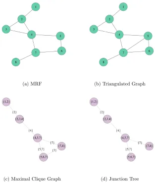
(a) MRF (b) Triangulated Graph

[image:26.612.171.484.86.456.2]

(c) Maximal Clique Graph (d) Junction Tree

Figure 2.2.2: Example of how a junction tree is calculated from an undirected network. Figure 2.2.2d shoes a possible junction tree for the MRF in Figure 2.2.2a.

from cliqueito clique j in the junction tree algorithm are defined as:

Mij(XSij) =

X

X_Ti_→_j\_Cj

Y

k:Ck⊂Ti→j

φk(XCk). (2.2.8)

Defining a root node in the junction tree, and then starting at the leaf nodes, the messages can be computed recursively. The messageMij(XSij) in (2.2.8) is equivalent to:

Mij(XSij) =

X

X_Ci\Sij

φ(XCi)

Y

k∈ne(i)\j

(27)

On completion of a sweep of message passing from the leaf of the tree up to the root and then back down again, all marginal probabilities can be calculated from the messages where the marginal distributions for the cliquesiis:

p(XCi)∝φ(XCi)

Y

k∈ne(i)

Mki(XSki). (2.2.10)

The junction tree algorithm for inference in MRFs is given in Algorithm 3. Observations can be incorporated into the algorithm by multiplying a single clique containing the involved random variables by the likelihood of the observation and completing a sweep on the message passing (Koller and Friedman, 2009).

Algorithm 3 Junction Tree Algorithm Setup:

1. Find the triangulated network

2. Find the junction tree using Algorithm 2 Run:

1. Choose a root node.

2. Pass messages from the leaves up to the root and then back down again, using (2.2.9). 3. Calculate desired marginals.

Computational Cost

(28)

Seymour, 1986).

In the best case, the tree width is small and the triangulated network which achieves this tree width is easy to find. In these cases, the junction tree algorithm provides a fast exact method for inference in graphical models (see Wainwright and Jordan (2008) for examples). However, in many cases, the graphical model is too complex and the tree width is too large for exact inference to be viable. In these cases, we rely upon approximate methods to perform inference in the graphical model.

2.3 Approximate Inference Methods for Graphical Models

A key obstacle in Bayesian inference is calculating marginal and posterior distributions. In an ideal setting, computing these can be done analytically, such as using the the junction tree algorithm for random variables in a graphical model. For large, complex data the computational costs associated with exact inference is too large. Instead, approximate inference algorithms are used to estimate the quantities of interest.

Exact inference algorithms can act as a starting point for approximate methods. These types of methods hope to use the structure of the graphical model to aid performance. They exploit situations where nodes or clusters of nodes are nearly conditionally independent, such as when node probabilities are well determined by only a subset of neighbouring nodes (Jordan et al., 1999). Pruning algorithms (Kjærulff, 1994), search based methods (Henrion, 1991) and localised partial evaluation (Draper and Hanks, 1994) have all been suggested to deal with these situations. Their advantage is that they still use the conditional independence properties exploited in the exact inference methods. However, they still suffer from many of the problems associated with exact inference, like the computational cost, which make exact inference difficult (Jordan et al., 1999).

(29)

Markov Chain Monte Carlo (MCMC) methods (Section 2.3.2). Both variational methods and Monte Carlo methods require the full specification of prior beliefs. In Section 2.3.3 we introduce Bayes linear methodology which can be used as an approximate inference technique when only a partial prior specification is required.

2.3.1 Variational Methods

Variational methods (Jordan et al., 1999; Wainwright and Jordan, 2008) are a popular group of approximate inference methods for graphical models. The methods can be applied to general probabilistic inference problems but their main application is in graphical models. The basic idea of variational methods is to characterise a probability distribution as the solution to a high dimensional optimisation problem, alter this optimisation problem and solve the altered optimisation problem.

Variational Bayes (VB) is a variational method for approximating the true distribution,

p(X), with the approximating distribution,q(X), where the closeness of the two distributions is measured through the Kullback-Leibler (KL) divergence. For a set of latent variables

X and observations Y, the interest may lie in the posterior distribution of the unknown variables given the observations:

p(X|Y) = p(X)p(Y|X)

p(Y) (2.3.1)

The VB approximation to the conditional distribution,p(X|Y) assumes a family of distri-butions,q(X)∈ D and approximates the distributionp(X|Y) by searching for q∗(X)∈ D which minimises the KL divergence:

KL(q(X)||p(X|Y)) =Eq[log(q(X)]−Eq[log(p(X|Y))]. (2.3.2)

(30)

used for inference. The complexity of the family of distributions determines the complexity of the optimisation; it is more difficult to approximate over a complex family than a simple family. As a result, a common variational family is the mean fields variational family, were the latent variables are assumed to be mutually independent:

q(X) =Y

i

qi(Xi). (2.3.3)

The idea for the mean fields approximation was adapted from statistical physics for inference in graphical model (Jordan et al., 1999; Attias, 1999).

The KL divergence,KL(q |p), is mainly considered for the computational advantages and can be seen to prefer q in areas of high probability under q. Hence, drawing samples and integrating with respect to q should be accurate but VB approximation may miss out on areas of high probability under p. Furthermore, whilst q will give a good approximation to the joint distribution, the marginals qi(Xi) should not be expected to resemble the true

marginals pi(xi) (Bishop et al., 2006). The approximation can be extended to include

dependencies between random variables, resulting in structured variational inference (Saul and Jordan, 1996).

(31)

An alternative class of algorithms is obtained by considering an outer approximation, where the set of parameters must satisfy a number of consistency relationships that arise from local neighbourhood relationships in the graph. A well used outer approximation is the belief propagation method in Section 2.2.1 when applied to graphs with cycles; called loopy belief propagation. It is a popular method due to its often remarkably accurate results (Murphy et al., 1999; McEliece et al., 1998). Loopy belief propagation is equivalent to a fixed point minimisation of the Bethe free energy equations for the graph (Yedidia et al., 2003). The Bethe approximation involves only those consistency relationships that rise from local neighbourhood relationships in the graphical model. There is no guarantee this algorithm will converge, and a large amount of theoretical and behavioural analysis has gone into understanding loopy belief propagation. Murphy et al. (1999) suggests that certain conditions, the approximation can often oscillate rather than converge. Koller and Friedman (2009) suggest several ways to help the loopy belief propagation work better. Algorithms known as cluster variational methods have been proposed to extend the Bethe approximation to higher order clusters of variables (Yedidia et al., 2003) along with other higher order variational methods (Leisink and Kappen, 2002; Minka, 2001).

(32)

2.3.2 Monte Carlo Methods

Monte Carlo methods rely on repeated random sampling from the distribution of interest to generate approximations to the true density. Consider a possibly multidimensional random variable, X, with probability mass function or probability density function, p(x), which is greater than zero for a set of values X. The expected value of some measurable function

g:X→Rd, with respect to the probability density p(x) is:

E[g(X)] =

Z

X

g(x)p(x)dx, (2.3.4)

ifX is continuous. The integral is replaced by a summation if the probability distribution is discrete. For a wide class of problems, it is not possible to evaluate the integral (or sum-mation) analytically. Monte Carlo methods represent a class of techniques where samples, simulated from the target distribution, can be used to approximate (2.3.4). Perfect Monte Carlo assumes samples can be drawn directly from the target distribution. If this is possible, taking n independent and identically distributed samples of X,

x(i) N_i₌₁, from p(X), the Monte Carlo estimate of the expectation ofg(x) is:

ˆ

g(x) = 1

N

X

i=1

g(x(i)). (2.3.5)

Monte Carlo methods are a simple appealing approximation technique with good statistical properties (Robert, 2004). The Monte Carlo estimator, ˆg(X) is an unbiased estimator of

E[g(X)]. Using the law of large numbers, ˆg(x) will converge almost surely to theE[g(X)] asN → ∞. Furthermore, the variance:

Var(ˆg(X)) = Var( 1

N

X

i=1

g(X(i))) = Var(g(X))

N , (2.3.6)

(33)

particular, those that are used in this thesis for inference.

Importance Sampling

In many situations, it is not possible to sample directly from the target distribution. This problem can be avoided by using an alternative sampling scheme. Importance sampling (IS) is a Monte Carlo method for evaluating integrals by drawing from a proposal distribution

q(x). The expectation of a function g(x), over the target distribution can be calculated over the proposal instead. The proposal is chosen to be easy to sample from, and must satisfy that if p(x) > 0 then q(x) > 0. The samples are weighted based on their fit to the target distribution; those with larger weights are more influential in the Monte Carlo approximation.

Using a proposal distribution (2.3.4) can be written as:

E[g(X)] =

Z

X

g(x)p(x)dx,

=

Z

X

g(x)p(x)

q(x)q(x)dx, =

Z

X

g(x)w(x)q(x)dx,

=E[w(X)g(X)], (2.3.7)

which is the expectation of w(X)g(X) with respect to the probability density q(x) and

w(X) =p(X)/q(X) is the importance weight. Sampling x(i) N_i₌₁ from the proposal distri-bution, the Monte Carlo approximation toE[g(x)] is:

ˆ

g(x) = 1

N

X

i=1

w(x(i))g(x(i)). (2.3.8)

(34)

whereZ is the unknown normalising constant. In this case:

E[g(x)] =

Z

g(x) p˜(x)

Zq(x)q(x)dx

≈ 1 ZN N X i=1 ˜

w(i)g(x(i)) (2.3.9)

where w(i) = p_q˜₍(_xx((ii)))₎ and the normalising constant is approximated using the Monte Carlo

sample as: Z≈ N X i=1 ˜

w(i). (2.3.10)

Using this, the normalised importance samples are:

ˆ

g(x) = 1

N

X

i=1

w(i)g(x(i)) (2.3.11)

where:

w(i)= w˜ (i)

PN

j=1w˜(j)

, i= 1, . . . , N. (2.3.12)

By the law of large numbers, (2.3.11) converges to E[g(x)]. However, the Monte Carlo estimate is biased, with decreasing bias as the sample size increases. The choice of pro-posal is important, as the variance of the estimator is dependent on the choice of propro-posal distribution (see Robert (2004) for information on the optimal proposal).

Monte Carlo Markov Chain Methods

(35)

interest. The method has been well studied and applied to several areas of statistics (Liu, 2008). A justification of this approach, and corresponding convergence properties can be found in Robert and Casella (2013).

A Markov chain is a collection of dependent samples,

x(1)_,_x(2)_{, . . .} _{, where the probability} ofx(n+1), given the samples at previous time steps, is only dependent onx(n):

p(x(n+1)|x(1), . . . ,x(n)) =p(x(n+1) |x(n)) =T(x(n),x(n+1)) (2.3.13)

and T(·,·) is known as the transition kernel. The target distribution is said to be the invariant distribution if the transition kernel satisfies:

X

x∗

T(x∗,x)p(x∗) =p(x). (2.3.14)

In this case, if the chain converges it will converge to the target distribution. Simulation from the Markov chain requires an initial distribution p(x(0)). After a suitable burn in period, the samples from the Markov chain are dependent samples fromp(x). If the Markov chain is irreducible and aperiodic, then:

1

N

X

i=1

g(x(i))→E[g(X)] (2.3.15)

with probability one asN → ∞.

The Metropolis-Hastings algorithm (Hastings, 1970) is a method to generate a Markov chain that will converge top(x) by successively sampling from an arbitrary proposal distribution

q(x∗ |x) and imposing random rejection steps at each transition. Let x(n) be the state of the MCMC algorithm after iterationn. To simulate the state at iterationn+ 1 a transition candidatex∗ ∼q(x∗ |x(n)) is simulated and with probabilityα(x(n),x∗):

α(x(n),x∗) = min

(

1, q(x

(n)_|_x∗_)˜_p₍_x∗₎

q(x∗ _|_x(n)_)˜_p₍_x(n)₎

)

(2.3.16)

(36)

The original Metropolis algorithm (Metropolis et al., 1953) was based on symmetry in the proposal distribution so that q(x | x∗) = q(x∗ | x). The advantage of the Metropolis-Hastings algorithm is that the target distribution is only required up to a normalising constant since this cancels out in the acceptance probability anyway. If the proposal,q(x|

x∗), is chosen to be positive everywhere, then the convergence top(x) is guaranteed (Robert, 2004). However, the rate of convergence depends on the relationship betweenq(x|x∗) and

p(x); choosing a q(x | x∗) which minimises the autocovariance results in a more accurate estimator with a finite sample.

The Gibbs sampler (Geman and Geman, 1984) is a method of simulating a Markov chain, by successively sampling from the full conditional distributions of the componentsp(xi |x−i)

wherex−idenotes all components ofxapart fromxi. The Gibbs sampler is a special case of

the Metropolis-Hastings algorithm where the acceptance probability is 1. At each iteration, each component of x(n) is updated. The ordering of the components can be random or deterministic (Liu, 2008). The difficulty in the method comes when the full conditionals are not of a standard form. Sampling methods, such as rejection sampling, can be used but often a Metropolis-Hastings sampler is used to provide the sample. Gibbs samplers are particularly applicable to problems of inference in graphical models. Using a MRF results in the full conditionals simplifying to conditionals dependent on only neighbouring nodes in the MRF and reduces the computation cost of computing them. A Gibbs sampler can be set up automatically from the graphical model specification (Gilks et al., 1994). Although the application of the Gibbs sampler naturally lends itself to inference in graphical model, the convergence of these types of models can be very poor. For some examples, where mixing is exponentially slow see Gore and Jerrum (1999).

(37)

a pseudolikelihood which is the product of normalised distributions over lower dimensional problems (Friel et al., 2009).

MCMC methods are computationally intensive methods. When a large computational cost is not an issue, MCMC methods can provide accurate samples from the posterior distribu-tion, providing asymptotically exact samples from the target distribution with convergence guarantees. However, the methods are less applicable to applications when the posterior distribution needs to be calculated quickly.

Sequential Monte Carlo Methods

The most widely used type of Monte Carlo methods are MCMC algorithms which can be applied to estimate the latent spacexconditional on observationsy. However, consider the situation where the aim is to track a sequence of distributions and estimate the posterior distribution. This type of online inference problem is not particularly well suited to MCMC methods. Each new observation would require simulating an entire new Markov chain for the new posterior distribution. Instead the samples from the posterior for x1:t−1 within an algorithm can be used to attempt to approximately samples from the posterior forx1:t.

Sequential Monte Carlo (SMC) methods can be used to do this by approximating a sequence of probability distributions on a sequence of probability spaces. The Monte Carlo techniques behind SMC have existed since the 1950s (Hammersley and Morton, 1954) but a lack of computational power at the time and problems with degeneracy meant these methods were generally overlooked. Since the introduction of the bootstrap filter (Gordon et al., 1993) and more general resampling schemes, there has been a large increase in research in this area. SMC works by taking an empirical approximation of the density using a collection of samples (also known as particles) and corresponding weights. The typical application is for inference in state space models, see Doucet and Johansen (2009) for applications of this type where the SMC models are more commonly known as particle filters.

(38)

distributionp(x0) and transition probabilities p(xt|xt−1):

p(x1:t) =p(x0)

t

Y

i=1

p(xi|xi−1). (2.3.17)

The observations at time t, are assumed to be conditionally independent given xt and the

joint distribution over both latent variables and observations is:

p(x1:t,y1:t) =p(x0) t

Y

i=1

p(xi |xi−1) t

Y

i=1

p(yi|xi). (2.3.18)

The aim is to recursively estimate the posterior distributionp(xt|y1:t) using a Monte Carlo

approximation:

ˆ

p(xt|y1:t) = N

X

i=1

w(_ti)δ_x(i)

t

(xt), (2.3.19)

whereδ(·) is the Dirac delta function andnw(_ti),x(_ti)

oN

i=1is the Monte Carlo approximation. Sequential Importance Sampling (SIS) is one way to sequentially calculate the Monte Carlo approximation. The approximation to the density is recursively updated as the new obser-vations are received, without modifying the previously simulated states. SIS propagates the particles in the Monte Carlo approximation from time t to t+ 1 and updates the weights accordingly, to give an approximation to the posterior density at timet+ 1. Suppose there is a proposal distributionq(x0:t|y0:t), which is easy to sample from, that has the property

p(x0:t|y0:t)>0 ⇒ q(x0:t|y0:t)>0 and can be updated recursively in time so that:

q(x0:t+1|y0:t+1) =q(x0:t|y0:t)q(xt+1|x0:t,y0:t+1). (2.3.20)

(39)

of proportionality is:

p(xt+1|y0:t+1)∝

Z

p(yt+1|xt+1)p(xt|y0:t)p(xt+1|xt)dxt,

=

Z _p₍_x

t|y0:t)q(x0:t|y0:t)

q(x0:t|y0:t)

p(yt+1|xt+1)p(xt+1|xt)q(xt+1|x0:t,y0:t+1)

p(yt+1|y0:t)q(xt+1|x0:t,y0:t+1)

dxt

(2.3.21)

Assuming there is a weighted Monte Carlo approximation at time t, nw_t(i),x(_ti)oN

i=1 to

p(xt|y0:t) then (2.3.21) can be approximated by propagating the set of particles to give

xi_t₊₁ N_i₌₁ and unnormalised weights:

˜

w_t(₊₁i) = ˜w_t(i)p(yt+1|xt+1)p(xt+1|xt) q(xt+1|x0:t,y0:t+1)

, fori= 1, . . . , N. (2.3.22)

The normalised weights are given by:

w(_t₊₁i) = w˜ (i)

t+1

PN j=1w˜

(j)

t+1

,

providing a weighted particle approximation to the marginal distribution at time t+ 1. The joint distribution to {x0:t+1} is approximated by storing the path of the particles

x0:t+1= (x0:t, xt+1) and still updating the weighting using (2.3.22).

Using the type of proposal distribution in (2.3.20), the weights of the particles can be sequentially updated in time, as the next observation becomes available. Assume it is possible to sample from the proposal distribution and both the likelihood and transitional probability are known. All that is needed is an initial set of samples to be generated. The proposal weights can be calculated sequentially. The SIS algorithm recursively propagates weights and particles as observation are received sequentially; it is given in Algorithm 4.

(40)

Algorithm 4 The Sequential Importance Sampling Algorithm

1. At timet= 0: (a) For i= 1, . . . , N

i. Samplex(₀i)∼p(x0)

ii. Evaluate the importance weights up to a normalising constant:

˜

w(₀i)=p(y0|x(0i)) (b) For i= 1, . . . , N normalise the importance weights:

w(₀i)= w˜ (i) 0

PN

j=1w˜ (j) 0

2. Fortin 1 to T

(a) For i= 1, . . . , N

i. Samplex(_ti)∼q(xt|x(ti−1) ,y0:t) and x(0:i)t= (x

(i) 0:t−1,x

(i)

t )

ii. Evaluate the importance weights up to a normalising constant:

˜

w_t(i) = ˜w(_t₋₁i) p(yt|x

(i)

t )p(x

(i)

t |x

(i)

t−1)

q(x(_ti)|x_0:(i)_t₋₁,y0:t)

(b) For i= 1, . . . , N normalise the importance weights:

w(_ti)= w˜ (i)

t

PN

j=1w˜ (j)

t

weight after running some iterations; a lot of work is devoted to updating particles which have almost zero weight. The degeneracy phenomenon is a big problem in SMC. A good choice of proposal distribution is key to slowing down degeneracy and can be found by minimising the variance of the particle weights. The optimal proposal distribution, first given by Zaritskii et al. (1975) is:

q(xt|x

(i)

t−1,y0:t)opt =p(xt|x

(i)

t−1,yt),

= p(yt|xt,x (i)

t−1)p(xt|x(ti−1) )

p(yt|x(t−1i) )

(41)

Substituting this into (2.3.20) gives:

w(_ti)∝w(_t₋₁i) p(yt|x(_t−1i) ). (2.3.24)

This means that the importance weights at timet can be calculated, and the particles pos-sibly resampled (with probability given by the weights), before the particles are propagated to time t. However, to use (2.3.23) it must be possible to sample from p(xt|xt(i−1) ,yt) and

calculate p(yt|x

(i)

t−1), one or both of which are often not possible (Doucet et al., 2000). A suboptimal choice of importance function must be used. The most popular choice is the transitional prior,p(xt|xt−1), which gives a weight w(ti) ∝w

(i)

t−1p(yt|xt). It is no longer

pos-sible to calculate the importance weights before the particles have been propagated at time

t. The auxiliary particle filter (Pitt and Shephard, 1999) tries to overcome this problem. At timet−1, the auxiliary particle filter tries to predict which samples will be in regions of high probability masses at time tby sampling each particle at time t−1 and propagating the sample forward to timet.

Degeneracy can also be minimised through a good choice of importance function and by including a resampling step in the SIS algorithm. The Sequential Importance Resampling (SIR), also known as the bootstrap filter (Gordon et al., 1993), was developed separately from the SIS algorithm and contains a resampling step at each iteration of the SIS algo-rithm. Since then, resampling has been shown to have both major practical and theoretical benefits (Doucet and Johansen, 2009). An IS approximation of the target distribution is based on weighted samples from q(xt−1|y0:t−1) and hence is not distributed according to

p(xt|y0:t). Resampling provides a way to give an approximation from the target

(42)

Algorithm 5 The Sequential Importance Resampling Algorithm

1. At timet= 0: (a) For i= 1, . . . , N

i. Samplex(₀i)∼p(x0)

ii. Assign weights ˜w(₀i)=p(y0|x (i) 0 ) (b) For i= 1, . . . , N

i. Normalise weightsw(₀i)= w˜

(i) 0 PN

j=1w˜ (j) 0

2. Fortin 1 to T

(a) For i= 1, . . . , N

i. Resample ˜x(_ti₋₁) by resampling fromnx(_ti₋₁) oN

i=1 with probabilities

n

w(_ti₋₁) oN

i=1 to give nx˜(_t₋₁i) ,_N1,oN

i=1

ii. Propagate weights ˜w(_ti)= p(yt|x(ti))p(x

(i)

t )

π(x(ti)|x

(i) 0:t−1,y0:t)

(b) For i= 1, . . . , N

i. Normalise weightsw(_ti)= w˜

(i)

t

PN j=1w˜

(j)

t

(43)

(Chopin, 2004; Douc and Moulines, 2007).

Sequential Monte Carlo in Graphical Models

Whilst the majority of approximate inference methods developed for graphical models are either variational methods or MCMC methods, recently there has been interest in how SMC can be used for the problem of inference in graphical models. Typically, SMC struggles in high dimensional problems (Rebeschini et al., 2015) and hence is not considered applicable to most graphical models. The first approaches that utilised SMC for graphical models use SMC within a loopy belief propagation framework (Isard, 2003; Sudderth et al., 2010). Even in the limit of the Monte Carlo sample size going to infinity, these methods are still approximate as they are taking approximations over loopy belief propagation.

As the dimension increases, the approximation to the target distribution quickly deteriorates when a single IS step is used (Bengtsson et al., 2008). The approximation error generally grows exponentially in the model dimension. However, this degeneracy can be avoided by starting off with a simple distribution and moving to the one of interest (Chopin, 2002). The stability of these problems is less well studied, although Beskos et al. (2014a) gives analytical understanding about the effect of dimension on SMC methods for static problems. The majority of SMC methods on graphical models work by slowly increasing the complexity of the graphical model to give a Monte Carlo sample which eventually approximates the full distribution for a static problem. For example, hot coupling (Hamze and de Freitas, 2005) starts with Monte Carlo approximation to a spanning tree of the MRF and edges are slowly added according to an annealing scheme. The method by Naesseth et al. (2014) works with the factor graph and sequentially adds factors to increase the probability space. As a byproduct of the algorithm, this also gives an unbiased estimate of the normalising constant. Both of these methods can be applied to discrete random variables and can be used within particle MCMC methods for parameter inference (Naesseth et al., 2014; Everitt, 2012).

(44)

on networks. Methods include those which break down the graphical model into smaller blocks. The SMC is independently performed on lower dimensional blocks before correcting for the blocking (Rebeschini et al., 2015; Briggs et al., 2013). By breaking the graphical model down, these methods are only approximations to the state space. Beskos et al. (2014b) introduces a space-time particle filter which uses a local particle filter in space and a global particle filter in time. Similarly, nested SMC (Naesseth et al., 2016) takes an exact approximation (Andrieu et al., 2010) to the weights in the SMC algorithm. The proposal distribution is the one used in fully adapted SMC. Instead of computing this proposal exactly, the weights are approximated by running an internal SMC sampler for each weight on the state space model, hence producing an unbiased estimate of the weights to move from time tto timet+ 1.

2.3.3 Bayes Linear Methodology

Variational Methods and Monte Carlo methods depend on a fully specified prior distribu-tion for the latent variables. For large complex data, it is often difficult to fully specify a prior distribution, which agrees with experts’ opinions (Craig et al., 1998). It may only be possible to specify partial prior beliefs. Instead of working with a full prior probability dis-tribution, an alternative is to use Bayes Linear (BL) methodology. This methodology works with the expectations directly rather than probabilities. Beliefs about the latent random variables are expressed through expectations and covariances rather than full probability distributions (Goldstein and Wooff, 2007) and these values are updated given observations. No assumptions are made about the underlying probability distribution of the model. The method of using subjective expectation to quantify expectations and uncertainty is some-times known as prevision. A rigorous development of the methodology for working directly with expectation as the primitive quantity is given in De Finetti (1974).

(45)

proba-CHAPTER 2. INFERENCE IN GRAPHICAL MODELS 35

bility of the event is given by the expectation of the indicator function.

BL methodology allows beliefs to be specified at the level of detail required through a set of random quantities, C = {X1, X2, . . .} where for each Xi, Xj ∈ C, the prior beliefs are

specified though:

• The expectation: E(Xi).

• The variance Var(Xi) quantifying uncertainty in the judgement of E(Xi).

• The covariance Cov(Xi, Xj) expressing the judgement of the relationship between the

random variables, quantifying the extent to which Xi may linearly influence Xj.

For example, for two random variablesX andY, interest may lie in the set of random quan-tities C =

X, Y, X2, Y2, XY . For each of these random quantities a prior expectation, along with variances and covariance would need to be specified to use BL methodology. An alternative way to specify a full probability distribution would be to specify the expectation of every possible combination of the random variables.

Formally, the belief specification is formed by constructing a linear spacehCiwhich consists of all finite linear combinations of the elements ofC. Covariance defines an inner product and norm over the linear space hCi. Hence, the name Bayes Linear follows from this linearity underlying the inner product structure. Operations which can be done on linear subspaces can be done in BL methodology. Familiar properties, present when working with probabilities, are also present when working within BL methodology such as linearity, convexity, scaling and additivity.

(46)

terms of minimising the mean squared error. LetY0 = 1, then the adjusted expectation is:

b

E[Xk|Y] = n

X

i=0

hiYi, (2.3.25)

which minimises:

E



 X_k−

n

X

i=0

hiYi

!2

, (2.3.26)

over all collections ofh= (h0, h1, . . . , hn) (Goldstein and Wooff, 2007).

This is a convex optimisation problem, and could be found using optimisation software. However, it is also possible to derive analytical equations for the best estimate. For any choiceh∗= (h1, . . . , hn), the value ofh0 is found by differentiating (2.3.26) with respect to

h0:

∂ ∂h0

Eh Xk−hT∗Y−h0

2i

= ∂

∂h0

E

X_k2

−2hT_∗E[XkY]−2h0E[Xk] + 2hT∗E[Y]h0

+hT∗E

YTYh∗+h20

,

=−2E[Xk] + 2h∗TE[Y] + 2h0. (2.3.27)

Then setting equation (2.3.27) equal to zero:

h0 =E[Xk]−hT∗E[Y]. (2.3.28)

For this value ofh0, the value ofh∗ is found by differentiating (2.3.26) with respect to h∗:

∂ ∂h∗

Eh Xk−hT∗Y−E[Xk] +hT∗E[Y]

2i

= ∂

∂h∗

Var(Xk) +hT∗Var(Y)h∗−2hT∗Cov(Y, Xk)

,

= 2hT∗Var(Y)−2Cov(Xk,Y).

Assuming thatVar(Y) is of full rank, setting this equal to zero gives:

(47)

and substituting into equation (2.3.25), the BL adjusted expectation is:

b

E[Xk|Y] =E[Xk] + Cov(Xk,Y)Var(Y)−1(y−E[Y]).

The adjusted variance ofXk givenY is:

d

Var(Xk|Y) =E

h

(Xk−Eb[X_k|Y])2 i

.

Substituting inEb(X_k|Y) from (2.3.29), the adjusted variance is: d

Var(Xk|Y) = Var(Xk)−Cov(Xk,Y)Var(Y)−1Cov(Y, Xk). (2.3.29)

The adjusted expectations and variances can be viewed as a primitive which quantifies aspects of the beliefs given observations. Alternatively they can be seen as a simple tractable approximation to a fully Bayesian analysis for complicated problems. For linear Gaussian models, the adjusted values are equivalent to the posterior mean and covariance found using a fully Bayesian analysis.

(48)

Chapter 3

Sequential Decision Problems

3.1 Introduction

In many real-world situations, decisions are made in order to help maximise some type of reward. The decisions are often difficult to make because of uncertainty in the system and about the outcome of the decision and any possible future outcomes. The decisions or the actions they generate do not only result in a reward but also result in new knowledge that can be used to help improve future decisions. This type of problem can be modelled as a sequential decision problem, which is a type of learning problem where the learning can be either offline or online (Powell and Ryzhov, 2012). In offline learning problems, no rewards are collected as the information is gathered. The decisions and feedback are sequential but a reward is only received at the end of the simulation. Ranking and selection is an example of an offline learning problem, where the concern is to find the best of two or more possible processes after a number of observations. See Kim and Nelson (2006) for an introduction to ranking and selection problems.

In online learning problems, the rewards are collected at the same time as information is gathered. Multi-armed bandit problems are one example of an online learning problem. They are one of the best known and most commonly used type of sequential decision problem

(49)

CHAPTER 3. SEQUENTIAL DECISION PROBLEMS 39

and arise in many different disciplines including statistics, operations research, machine learning, computing, control theory and economics. One of the original motivations for studying the multi-armed bandit problems coming from statistics was the sequential design of experiments (Robbins, 1952).

Sequential decision problems have been extensively studied because of the large number of applications. Different disciplines vary in their approach to these types of problems, driven by differing motivating applications. Machine learning has recently been very active in the area of research for multi-armed bandits. For example, in website optimisation (Scott, 2010), where the observations are easy to observe and the outcome is almost instantaneous, they combine the ideas of sequential learning motivation (Robbins, 1952) with ideas from reinforcement learning; the process of learning about uncertain environments and observing the outcomes inspired by behavioural psychology (Sutton and Barto, 1998). Many of the applications within statistics and operations research have less instantaneous rewards and a higher cost associated with them. For example, deciding where to drill to find oil, or deciding which drug to give a patient in a clinical trial.

3.1.1 Markov Decision Processes

A common way to model a sequential decision problem is as a Markov Decision Process (MDP), a discrete time stochastic process which is an extension of a Markov chain with the addition of actions and rewards. A detailed introduction to MDP is given in Whittle (1982) and Puterman (2014). The process moves through the states with some transition probability, which depends on the actions of the decision maker. Hence, the transition probability depends on the current state of the system as well as the action. Given the current state and action, the next state is conditionally independent of all previous states and actions. Hence, the state transitions satisfy the Markov property.

(50)

time horizons, the rewards are usually discounted by a fixed factor so that the total reward is finite. An action will not only be determined by the possible immediate reward but also any possible future rewards. For example, an action may result in a poor immediate reward but lead to good future rewards. Hence, evaluating the current best action results in looking at all possible future actions.

The multi-armed bandit problem is an example of a one state MDP, where learning is added to the problem (Vermorel and Mohri, 2005). This occurs when transition probabilities are not fully known and can be learnt from the outcome of the actions.

3.1.2 Multi-armed Bandits

A typical example of a multi-armed bandit problem is the problem of a gambler at a row of slot machines (sometimes called one-armed bandits). The gambler must decide which machines to play, how many times to play them and in which order they should be played. The objective of the gambler is to maximise the sum of their rewards over the sequence of plays. More generally, in a classical multi-armed bandit problem, the decision maker faces

Kpossible actions (also known as arms). Associated with each possible action are unknown parameters,θa∈Θ. At each time step,t= 1,2, . . . an action ak ∈ {1, . . . , K} is taken and

the action at =a corresponds to choosing actionsa at time t. This results in an observed

rewardyt, which is assumed to be drawn from the marginal distribution νawith parameters

θa:

Yt∼νa(θa). (3.1.1)

The expectation of the reward on armaat timet is denotedµa:

E[Yt] =µa. (3.1.2)

From a Bayesian point of view, the parameter values (θ1, . . . , θK) are drawn from a prior

(51)

reward over the time horizonn:

E

" _n X

i=1

Yt

#

(3.1.3)

over both the realisations and the prior information. For an infinite time horizon, the reward is multiplied by a discount factor,γ, and the policy is chosen which maximises:

E

"_∞ X

i=1

γtYt

#

. (3.1.4)

In the past couple of decades, many algorithms have been suggested for determining the best policy for the multi-armed bandit problem. These problems can be seen as a type of exploration-exploitation problem. At each stage, there is a trade-off between sampling a reward on an arm which appears to be doing well based on the limited information of previous rewards (exploitation) and sampling a reward on an arm which may look inferior because of sampling variability (exploration) (Auer et al., 2002). A simple heuristic policy is the greedy policy where at each time step, the action with the highest posterior expected reward,µj,t, is picked:

at= argmaxj=1,...,Kµj,t. (3.1.5)

The method can be seen as a pure exploitation method. Better methods will combine both exploration and exploitation in order to maximise the future rewards. Section 3.2 gives details of some alternative policies.

3.2 Solutions

(52)

solution to the multi-armed bandit problem reduces to an index problem. An index is a numerical value independently assigned to each of the arms and the policy is chosen by selecting the arm with the highest index. Gittins and Jones (1979) proved that the optimal policy for the infinite horizon multi-armed bandit problem, with discounted rewards where the rewards are conditionally independent given the action, is an index policy. They termed the index the dynamic allocation index but it is now commonly referred to as the Gittins index. Easier to follow proofs have since been given to show that Gittins index is optimal for multi-armed bandit problems (Tsitsiklis, 1994). One way the Gittins index can be derived is by considering a smaller independent problems for each arm where the arm is pulled and it must be decided adaptively when to stop pulling that arm. Upon stopping a fixed retirement cost is given. The Gittins index is the arm with the largest fixed retirement cost required to stop pulling the arm now (Frazier, 2011). The solution is reduced from solving a k-armed bandit problem to solving the Gittins indices for k one-armed bandits. For many problems these optimal policies are hard to compute, and for finite horizon problems Gittins indices are no longer optimal; the proof is fragile to changes in the assumptions. As a result, research has turned to heuristic methods which are not guaranteed to select the optimal policy at each time step to solve multi-armed bandit problems.

An alternative way to measure how well a decision policy performs is to minimise the cumulative regret (Robbins, 1952). Ifµ∗ is the maximum expected reward over theK arms then instead of maximising the cumulative reward, the multi-armed bandit problem can be thought of as minimising the cumulative regret:

Rn(θ) = n

X

t=1

(µ∗−µat). (3.2.1)

A basic objective given by Robbins (1952) is thatRn(θ)/n→0 as n→ ∞. Policies which