Experimental and Theoretical Developments in Extended X Ray Absorption Fine Structure (EXAFS) Spectroscopy

EXPERIMENTAL AND THEORETICAL DEVELOPMENTS IN EXTENDED X-RAY ABSORPTION FINE STRUCTURE (EXAFS) SPECTROSCOPY

Thesis by John James Boland

In Partial Fulfillment of the Requirements for the Degree of

Doctor of Philosophy

California Institute of Technology Pasadena, California

1985

i i

i i i

ACKNOWLEDGEMENTS

I have enjoyed my stay at Caltech and I would like to take this opportunity to thank those who made i t such a pleasant experience. To my thesis advisor, Dr. John D. Baldeschwieler, I owe a great debt of gratitude for his support and encouragement throughout my years at Caltech. John has given me an insight into the worlds of science and business which I will take with me through life. I would also like to thank the members of the JDB group with whom I have worked with over the years. In particular, I would like to thank Dr. Folim G. Halaka who worked closely with me on the EXAFS project. Thanks is also due to our secretary Susan Shaar who typed many boring manuscripts and also to the staffs of the electronics and machine shops for their assistance in times of difficulty.

iv

ABSTRACT

To obtain accurate information from a structural tool i t is necessary to have an understanding of the physical principles which govern the interaction between the probe and the sample under investigation. In this thesis a detailed study of the physical basis for Extended X-ray Absorption Fine Structure (EXAFS) spectroscopy is presented. A single scattering formalism of EXAFS is introduced which allows a rigorous treatment of the central atom potential. A final state interaction formalism of EXAFS is also discussed. Multiple scattering processes are shown to be significant for systems of certain geometries. The standard single scattering EXAFS analysis produces erroneous results if the data contain a large multiple scattering contribution. The effect of thermal vibrations on such multiple scattering paths is also discussed. From symmetry considerations it is shown that only certain normal modes contribute to the Debye-Waller factor for a particular scattering path. Furthermore, changes in the scattering angles induced by thermal vibrations produces additional EXAFS components called modification factors. These factors are shown to be small for most systems.

v

CHAPTER I:

CHAPTER II:

vi

TABLE OF CONTENTS

Acknowledgments •••••••••••..••••.••••.. i i

Abstract

. . .

.

. . . .

. .

.

. .

.

iv Table of Contents . . . . vi List of Illustrations and Figures •••••• ix Introduction to Extended X-ray Absorption

Fine Structure (EXAFS) Spectroscopy •••• References

...

Theory of Extended X-ray Absorption Fine Structure: Single and Multiple

Scattering Formalisms

1 7

Introduction ••••.••••••••••••••••.•...• 8 The General Formalism

. .

.

. .

.

.

. .

. . .

. .

.

10 The Single Scattering Formalism •••••••• 13 The Multiple Scattering Formalism •••••• 19 Results and Discussion • • • • • • • • • • • • • • • • . 26

Appendix A 33

Appendix B 34

References

.

.

. . . .

.

. . .

.

. . .

. .

. . .

.

. .

36 CHAPTER III: Theory of Extended X-ray Absorption

Fine Structure: Final State Interaction Formalism

Introduction •••••••••••••••.••••••••••• 51 Final State Interactions • • • • • . . • • • • • • • • 52 The Jost Function Formalism .•..••••.••• 55 The EXAFS Regime ••••••••••••••••••••••• 60 Analytical Properties of the Jost

vii TABLE OF CONTENTS (continued) CHAPTER IV:

CHAPTER V:

CHAPTER VI:

The Effect of Thermal Vibrations on Extended X-ray Absorption Fine

Structure: Debye-Waller Factors

Introduction ••••••••••••••••••••••••••• 69 The General Formalism •••••••••••••••••• 70 The EXAFS Problem •••••••••••••••••••••• 75 Application to Model Systems ••••••••••• 80 Discussion

References

. . .

.

. . .

.

.

. .

The Effect of Thermal Vibrations on

Extended X-ray Absorption Fine Structure: Modification Factors

88

97

Introduction . . • . . . . 111

Formal Considerations •••••••.•.•...••.. 114 EXAFS Modification Factors ••••..•..•••• 121 Application to Model Systems ••••.•.•••• 128 Discussion

References

The Ca1tech Laboratory EXAFS Spectrometer

Introduction

General Description of the

133 146

162

Spectrometer •••••••.••••••••••••••..••. 164

X-ray Source 167

Monochromator System • • • • • • • • • • • . • • • . . . . 170 X-ray Detectors •••••••••••••••••••••••• 172 Spectrometer Performance . . • • . . . • • . • • • 173

Conclusions . . . . 176

viii

TABLE OF CONTENTS (continued)

CHAPTER VII: Data Analysis in Extended X-ray Absorption Fine Structure: Determination of the Back-ground Absorption and the Threshold Energy

Introduction 185

Experimental Approach ••••..••••••.••••• 188 Computational Approach ••••••••••••••••. 191

Discussion 194

References

. . .

. .

. . . .

.

.

.

.

.

. .

. . .

. . . .

. .

.

200 CHAPTER IIX: Identification of Neighboring Atoms in

Extended X-ray Absorption Fine Structure

CHAPTER IX:

Introduction ••••.•••••••••••••••••••••• 209 Physical Basis for the Atom

Identification Scheme •••••••••••••••••• 211 Data Acquisition and Analysis •••••••••• 211 Results and Discussion . • • • • • • • • • . • • • • • • 217

References • . • • . • • • • . • • • • • . . . • • • • • . . . • • . 228

Possibility of Bond-Length Determination in EXAFS without the Use of Model Compounds or Calculated Phases

Introduction . . . . 243

Physical Basis for the Method ....•••••• 244 Application to Model Systems ••.•••••.•. 249 Discussion

. . .

. . .

. .

. . .

. .

. . .

. . .

252

ix

LIST OF ILLUSTRATIONS AND FIGURES CHAPTER II

Figure 1.

Figure 2.

Figure 3.

Figure 4. Figure 5.

Figure 6.

Figure 7.

Figure 8.

Figure 9.

Figure 10.

Schematic representatrion of the

final state potential •••••••••••••••• 39 Diagrammatic representation of the

first and second order terms in the

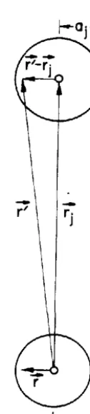
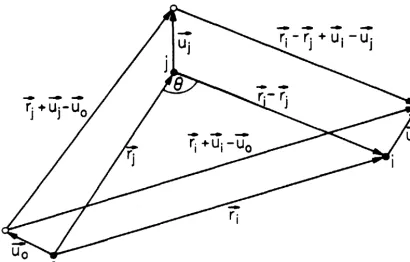
expansion of the full T operator ••••• 40 The vectors pertaining to the evaluation of the Green's function ••••.••••••••• 41

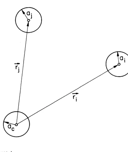
The three-atom system . . . • . . • • • • • • • • • •

The most significant scattering paths within the three-atom system •••••••.• Schematic representation of the terms

in the EXAFS expression for the

three-42

43

atom system • • • • • • • • • • • • • • • • • • • • • • • • • • 44

Calculated EXAFS spectra for the

Fe-0-Fe system . . . 45

Calculated EXAFS spectra for the

Cu-s-cu system . . . • • • . . • . . • . . . • . . • • . 46

Representative Fourier transforms of the bridged iron and copper systems ••••.• 47 Peak positions

transform as a bridging angle

in the Fourier function of

48 Figure 11. Relative amplitudes of the peaks in

the Fourier transform as a function

of bridging angle ••••••••.•••••••••.• 49 Figure 12. Amplitude enhancement and the error in

the distance from an analysis of a

~-oxo bridged iron system •••••••••••• 50 CHAPTER IV

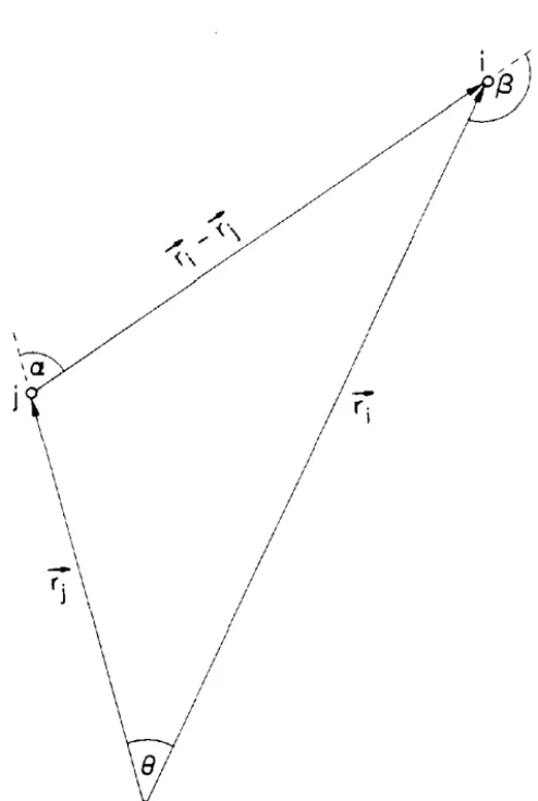
Figure 1. The general three-atom system •••••••• 99 Figure 2. The five significant scattering paths

X

LIST OF ILLUSTRATIONS (continued)

Figure 3.

Figure 4.

Figure 5.

Figure 6.

Figure 7.

Figure 8.

Figure 9.

Table I

CHAPTER V

Figure 1.

Figure 2.

Figure 3.

Figure 4.

Figure 5.

Figure 6.

Figure 7.

Figure 8.

Schematic of the normal modes in a

three-atom system of

c

_{2v symmetry ••••} 101

Schematic of the normal modes in a

three-atom system of D~h symmetry •••. 102

The symmetrized normal coordinates 103

Calculated Debye-Waller factors as

a function of bridging angle .•••••••• 104

Normal frequencies for BeBr 2 as a

function of bridging angle ••••••••••• 106

Temperature dependence of the

Debye-Waller factor for BeBr 2 ••.••.••....•. 107 Modification in the EXAFS amplitude due

to Teo's assumption •••••••••••••••••• 109

Normal frequencies of vibration for a

series of linear systems ••••••••••••• 110

The general three-atom system 148

The five significant paths in a

system of three-atoms ••.••••••••••••• 149

Schematic of the normal modes of

vibration for a

c

_{2v system ...} 150

Schematic representation of the vectors which determine the change in angle due to the displacement of all of the

atoms in a given normal mode ••••••••• 151

Frequencies of the normal modes for

the Br 2

o

system •••••••••••••••••••••• 152

Debye-Waller factors for the Br 2o

system • • • . • • • • • • • • • • • • • • • • • • • • • • • • • . . 153

The argument of the hyperbolic sine terms for the double and triple

scattering paths ••••••••••••••••••••• 154

Modulus o: the scattering amplitude

xi

LIST OF ILLUSTRATIONS (continued)

Figure 9. Phase of the scattering amplitude

for oxygen . . . . 156

Figure 10. Amplitude of the individual terms

which contribute to the EXAFS of

the Br 2

o

system at 10 K •••••••••••••• 158

Figure 11. Amplitude of the individual terms

CHAPTER VI

Figure 1.

Figure 2.

Figure 3.

Figure 4.

Figure 5.

Figure 6.

CHAPTER VII

Figure 1.

Figure 2.

Figure 3.

Figure 4.

Figure 5.

Figure 6.

which contribute to the EXAFS of

the Br 2

o

system at 300 K ••••••••••••. 160

Schematic of the laboratory EXAFS

spectrometer •••••••••••••••.•....•••. 179 A scaled drawing of the laboratory

spectrometer •••••••••••••.••..•...••. 180 The Johansson monochromator

configuration ••••••••••••••..•••..••. 181

Crystal bending apparatus with two

bending moments •••••••••••••••••••••• 182

Schematic of a parallel plate

ionization chamber . . • . . . • • . . . . 183

The copper Ka doublet • • • • • • • • • • • • • • • • 184

Spectral distribution of energies diffracted by the monochromator

at 9500 ev . . . . . . 202 Plot of the absorption as a function

of x-ray energy for a copper foil

Plot of the post-edge absorption as a function of the wavenumber of

203

the photoelectron . . . • . 204

Plot of the original EXAFS and the

calculated background •••••••••••••••• 205

Plot of the EXAFS as a function of

photoelectron wavenumber ••••••••••••• 206

Modulus of the Fourier transform for

xii

LIST OF ILLUSTRATIONS (continued)

Figure 7.

CHAPTER VI II

Figure 1.

Figure 2.

Figure 3.

Figure 4.

Figure 5.

Figure 6.

Figure 7.

Figure 8.

Table I

Table II

Table III

CHAPTER IX

Figure 1.

Table I

The background and the threshold energy determination using the

computational approach ••••••••••••••• 208

The scattering phases for carbon

and oxygen ••••••••••••••••••••••••••• 230

Determination of the threshold energy

for Co(acac} 3 •••••••••••••••••.•••••• 231

Isolated EXAFS spectra ••••••••••••••• 232

Modulus of the k3 weighted

Fourier transform ••••.•..•••••••••••. 234

Total phase from the first-shell peaks

of the Fourier transform .••••••••.••• 236

A comparison of the new windowing

method with earlier methods •••••••••• 237

The EXAFS and the Fourier transform

from the [Co(NH 3 } 6 ]Cl 3 complex ••••••• 238 Phase intercept for a coordination

shell made up of two kinds of atoms 239

The coefficients from the

least-squares fit to the total phase ••••••• 240

The coefficients from the least-squares fit to the total phase

for the amine complex • • • • • • • • . • • • • • • • 241

Calculated phase intercepts for

a two component system •••••••••..•... 242

Plot of the total phase and the

function g 1 (k) as a function of k • • • • 254 The parameters obtained from a

1

CHAPTER I

INTRODUCTION TO EXTENDED X-RAY ABSORPTION

FINE STRUCTURE (EXAFS) SPECTROSCOPY

The term extended x-ray absorption fine structure

(EXAFS) refers to the modulations in the x-ray absorption

coefficient which occur on the high energy side of an

absorption edge. The first experimental observation of

these oscillations was made by Fricke 1 and Hertz2 in 1920.

The observed structure was confined to the near edge

region3, howev€r, and thus could be readily explained by the

theory of Kossel. 4 As experimental measurements improved,

the structure was seen to extend many hundreds of electron

volts past the edge with an amplitude of approximately 10%

of the edge itself. Accordingly, a new description of this

phenomenon was required.

An explanation of the physical basis of the EXAFS

effect in condensed matter was first proposed by Kronig.s

In this case, the EXAFS was described in terms of a

modification of the final state photoelectron or Bloch wave

due to scattering at the boundary of the Brillouin zone.

Since this description depends explicitly on the periodicity

of the solid such an explanation became known as a long

range (LRO) theory of EXAFS. To explain the observation of

EXAFS in molecules Kronig also proposed6 a short range order

(SRO) theory, in which the final state photoelectron wave is

2

realized that the same basic physics could be used to explain the observation of EXAFS in both solids and molecules. Indeed, as late as 1963, there was still a great deal of confusion as to which theory was the most appropriate description of EXAFS. 7 A major source of this confusion was the lack of quantitative comparison between theory and experiment.

It is now generally accepted that, in most instances, a single scattering SRO theory is an adequate description of

EXAFS. The normalized oscillatory component of the

absorption coefficient above a K-edge may be expressed as: X(kl ,. z:ce.rjl2Nj1fj(k,lT)

I

sin(2krj + ej>

j krj

(1.1.1) This equation describes the modification of the photoelectron wave, which originates from an absorbing atom which is situated at the origin, and is scattered by Nj neighboring atoms at a radial distance rj away. The amplitude of the EXAFS oscillations is dependent on the ability I fj(TI,k) I of these atoms to backscatter the photo-electron. Note that the EXAFS is expressed in terms of the photoelectron wavenumber k which is defined by k:[2m(hw-E

0 ) ]

1

₁

_{2;h, where flw is the x-ray energy and E}

3

phase shift due to scattering off both the absorbing and

neighboring atoms. As suggested by Schmidt,9 a term to

account for thermal vibrations and static disorder should be

appended to Eq. (1.1.1). Furthermore, since electrons which

suffer inelastic losses may not contribute to the EXAFS, a

mean -free path damping term must also be included in Eq.

l 10

( . l . l ) .

The present interest in EXAFS began with the work of

sayers, Stern and Lytlell who realized that if Eq. (1.1.1)

is a valid description of the EXAFS, then it should be

possible to invert this expression to obtain the distances

rj. In particular, they showed that a Fourier transform of

Eq. ( l . l . l ) is a form of radial distribution function in which the absorbing atom is located at the origin.

Accordingly, there is a peak in the transform associated

with each shell of atoms surrounding the central atom.

These peaks do not occur at the true shell distances due to

the presence of the phase function 9j(k) in the argument of

each sine wave. Therefore, to obtain distance information

from EXAFS the k dependence of these phase functions must be

known. If in addition, coordination numbers are to be

determined, some information on the scattering amplitudes is

required, together with a knowledge of the Debye-Wallerand

inelastic damping factors. In practice, however, model

compoundsl2 and theoretical calculations 1 3 are used

extensively to extract structural information from EXAFS

4

The increased understanding of the physical basis of the EXAFS effect has been paralleled by a rapid development in the instrumentation used to measure EXAFS spectra. In particular, the advent of synchrotron radiation sources has provided a major impetus for the development of EXAFS as a structural too1. 14 Furthermore, high flux laboratory spectrometers, which utilize rotating anode sources and large crystal monochromators, are now available These advances allow high signal to noise EXAFS spectra to be obtained in an acceptable period of time.

In view of these developments, i t has been our objective to carefully re-examine the physical basis for the EXAFS effect. In Chapter II we have introduced a rigorous scattering formalism for EXAFS, which accounts for the presence of the central atom potential in a quantitative manner. The formalism also demonstrates the close relation-ship between EXAFS and the modulations observed in electron yield experiments. The contribution of multiple scattering processes to the observed EXAFS, which was neglected by earlier workers, is shown to be significant for systems of certain geometries • In such instances, the standard single scattering analysis methods are shown to be no longer valid. However, a careful study of such multiple scattering data should allow bond angles to be determined.

A formalism, which does not explicitly. involve a scattering

III. This

description of scheme allows

5

EXAFS in terms of the overlap between the initial and final states. At sufficiently high energies this description reduces to the standard EXAFS expression, Eq. (1.1.1). Unlike earlier theories, this formalism is valid over the complete energy range and may be used to describe both bound state transitions and shape resonances. Furthermore, the expression for the final state structure is an analytic function of k, and hence, may be used to calculate the damped or imaginary component of the photoelectron wave.

Since multiple scattering effects may contribute significantly to the EXAFS, the simple treatment of the thermal vibration given by Schmidtg is no longer valid. In Chapters IV and V of this thesis we discuss in detail the effects of thermal vibrations on EXAFS. The correlated motion of the atoms involved in the scattering process is explicitly calculated. The manner in which one should analyze such data is also discussed.

6

bond distances from EXAFS data without the use of model

7

References

1. H. Fricke, Phys. Rev. 16, 202 (1920).

2. G. Hertz, Zeit. f. Physik, 3, 19 (1920).

3. A.E. Lindh, Zeit. f. Physik, 6, 303 (1920).

4. W. Kossel, Zeit. f. Physik, 1, 119 (1920).

5. R.L. Kronig,

z.

Physik, 70, 317 (1931).

6. R.L. Kronig,

z.

Physik, 75, 468 (1932).

7. L.V. Azaroff, Rev. Mod. Phys. 35, 1012, (1963).

8. H. Peterson, Zeit. f. Physik, 80, 528 (1933).

9. V.V. Schmidt, Bull. Acad. Sci. USSR, Ser. Phys. 25, 998 (1961); 27, 392 (1963).

10. M. Sawada, Rep. Sci. Works Osaka Univ. 7, 1 (1959).

11. O.E. Sayers, E.A. Stern and F.W. Lytle, Phys. Rev. Lett. 27, 1204 (1971).

12. P.H. Citrin, P. Eisenberger and B.M. Kincaid, Phys. Rev. Lett. 36, 1346 (1976).

13. P.A. Lee and G. Beni, Phys. Rev. B 15, 2862 (1977).

14. B.M. Kincaid and P. Eisenberger, 1361 ( 1975).

8

CHAPTER II

THEORY OF EXTENDED ~-RAY ABSORPTION FINE STRUCTURE: SINGLE AND MULTIPLE SCATTERING FORMALISMS*

2.1 Introduction

Beginning with Kronig in 1932, a number of short range

order theoriesl-11 have been proposed to explain the

post-edge fine structure--the extended x-ray absorption fine structure or EXAFS--of the x-ray absorption edge (see reviews of this subject by Lee et ~.,12 Sternl3 and With the exception of Lee's recent worklo, all these studies suffer from difficulties in their treatment of the outgoing photoelectron wave, the scattering potential, or the central atom phase shift. Nevertheless, each study arrives at essentially the same expression for the oscillatory component of the K-edge x-ray absorption cross section:

x(k)"' IJ.-IJ.o =-

2,)e.

1)2 lf(rr,2k) I

!J.o ₁ kr₁

xsin[2kr₁ + 21i₁(k) + ())(k)]. (2.1.1)

where the symbols have the following meanings: k=[2m(flw-E

9

The phase shift due to the central atom potential is 2

o

_{1 , and} u (k) and u₀ (k) represent the absorption coefficients in the presence and absence of neighboring atoms in the final state.

In the case of polycrystalline samples, the geometric factor (e.rj)2, averages to a constant. Additional terms, to account for thermal effects 1 5 and losses due to inelastic scatteringS, may also be appended to Eq. (2.1.1)

HJ

scattering formalism. In fact , the form of the E XA F

s

expression assumed by Teo 2 8 is incorrect, since i t neglects a geometrical factor which does not average out in polycrystalline materials (see Section 2.5).

In this chapter we discuss an approach which separates the single and multiple scattering contributions of the general problem, and develops computational methods applicable to both. A general three-atom formalism is developed and employed in the discussion of two physically significant model systems.

2.2 The General Formalism

The x-ray absorption cross section in the dipole and the one-electron approximations is given by:l6

(2.2.1)

where a is the hyperfine constant, w is the angular photon frequency, and N(w) is the density of final states for the photoelectron. The initial and final states of the system (i and f) are both eigenfunctions of an approximate unperturbed Hamiltonian H:

n

2 _Ze2

H - - - v2_{- - + v}

- 2m r r (2.2.2)

11

the absorbing or central atom c. A schematic representation

of this final-state potential is shown in Fig. 1. The

potential energy between the atomic sites is assumed to be

constant and represents the zero of energy in the system.

In order to calculate the matrix element in Eq.

(2.2.1), i t is necessary to find the appropriate

eigenfunctions of H. At energies corresponding to bound

K-shell electrons (the only initial state considered here),

the potentials of the neighboring atoms may be ignored, and

the eigenfunction of the resulting Hamiltonian is the usual

hydrogenlike wavefunction:

(

z

)3/2

(rli)=rr"112

ao

exp(-Zr/a0) _(2.2.3)

Two factors influence the nature of the final state:

the potentials of the neighboring atoms and that due to the

central or absorbing atom. For photoelectrons of

sufficiently high energy (approximately three times the

plasma frequency 6 ), the attractive potential of the central

atom's nucleus, together with the influence of the other

bound electrons (though these are not explicitly considered

here), becomes negligible, and the Schrodinger equation

reduces to:

(2.2.4)

where H0 _{is the free-particle Hamiltonian. This equation}

12

(2.2.5)

where <rlk> are the normalized eigenfunctions of H0 • We

shall use the minus form of Green's and T operators, so that

<rlk> corresponds to the outgoing asymptote of the

scattering process described by <r If>. The description of

the EXAFS phenomenon is thus expressed in terms of the state

of the photoelectron after the scattering process is

complete. Furthermore, this choice of asymptote most

clearly illustrates the close relationship between EXAFS and

the modulations observed in electron-yield type

experi-ments.29

The full T operator may now be expanded in terms of the

operators tj associated with the individual scattering

centers located at r=r·lB J

(2.2.6)

Note that successive scattering by the same potential is not

permitted.

Substitution of the first two terms of Eq. (2.2.6) into

the Eq. (2.2.5) yields an expression which may be

represented graphically as shown in Fig. 2. The first

diagram in this figure represents the simplest single

scattering case: a photoelectron ejected in the direction

i'j, and scattered in some direction R by the atomic

potential at r=rj. A similar interpretation applies to the

13

scattering processes in which the photoelectron is scattered successively by two atomic potentials.

In particular, the third and fourth diagrams in Fig. 2 represent processes for which the second scattering center is the absorbing atom potential. In such instances the scattering path length is identical with that in the corresponding single scattering process. Accordingly, such terms must also be considered within our single scattering theory. The term corresponding to secondary scattering by the absorber was first discussed by Lee 10 and allows a rigorous treatment of the effect of the central atom potential. The approach adopted, however, was not sufficiently general to be readily extended to multiple scattering problems.

2.3 The Single Scattering Formalism

The two single scattering terms of Eq. (2.2.6) may now be substituted into the matrix element in Eq. (2.2.1):

<J-

I

e.

r

I

i>

=

<k

I

e ·

r

I

i/

+

.l)k

I

tjG;e ·

r

I

i>

i

+

L

(k I

t;G;t;G;e ·

r I i) ,

(2.3.1)

J

where we have taken the complex conjugate of Eq. ( 2.2.5) and

*

have noted that t(z )=[t(z)]t.

The first matrix on the r:ight-hand side of Eq. (2.3.1) is responsible for the usual unperturbed photoelectric effect (i.e., for 11₀ ) , and is evaluated in Appendix A with

14

(kle·

rli>=M(k,Z)k·

e,

.

(z

)s'2

M(k, Z)

~

- (2 )'";

(;:o

)3 .

1T - + k2

ao

(2.3.2)

The remaining terms in Eq. (2.3.1) may be expanded in a complete set of states to obtain:

L

(k

I

t;c~e

·

r

I

i)

J

=

L:f<k

I t;lrt><rtl c;l

r>

e ·

r<rli> drdrt

J

(2.3.3)

and

L

(k

I

t;c;t;c;e ·

r I i) =

L

J<k

It; I r3)(rsl

c;

I

r2>

J J

(2.3.4)

X (r21

t;

I

Yt)(rl

I

c;

I

r)

e.

r(r

I

i) dr drt dr2 drs

15

All that remains now is to evaluate matrix elements of the forms:

(r'IGolr>

and

(r'lt;!r).

The configuration-space matrix element of the Green's operator are given by the corresponding free-particle Green's function:

e'•lr' -rl

(r'IGolr>=-

2~2

lr'-ri · (2.3.5)

Note that

I

r

I

in Eq. (2.3.5) is of the order of a

0/Z or less while r' is restricted to a domain of radius aj around rj (see Fig. 3). Hence r'"" rj and

I

r'-rl may be expanded as:l9

(2.3.6)

Therefore, the Green's function in Eq. (2.3.5) may be approximated by:

(r' I G

₀

lr>

~

-2m"' _rr" 2 ...!:_ _r exp(ik1 • (r'- r)] ,

1

(2.3.7)

the direction of propagation of the photoelectron. The error in making this approximation, aj/rj, is small since the core electrons of the neighboring atoms are responsible for most of the scattering in the EXAFS energy regime.12

16

described in Appendix A, with the results:

(2.3.8)

L

(k

I

t;c;t;c;e ·

r

I

i) =

L

m~~rr)

4

_;.M(k, Z)(e.

1)

J J rj

X (kIt~

I

k;)(k;

I t;l

kJ) '

(2.3.9)

where

k)

=-krj is the direction of propagation of the back-scattered photoelectron.

We may now relate the matrix elements of tj<rj) to those of tj(O) which represent the identical scattering problem, but centered about the origin20

Since only elastic scattering events (i.e., lkl=lkjll are of interest, the matrix elements of tj(O) form an on-shell T matrix which may be expressed in terms of the scattering amplitude fj(9j):21

(2.3.11)

where cosej=R.Rj=R.rj.

17

(3. s) =L:M(k,

z).!.(e ·

1)fJ(eJ)

J YJ (2.3.12)

xexp(ikrJ(1-cos81) ] ,

and

(3. 9) = LM(k, Z)

~

(e • 1)!₁(rr)

J

rJ

(2.3.13)

X/₀(7r-il₁)exp(2ikrJ) ,

where cos(n-ej)=R.R1=-R.rj.

The complete matrix element in Eq. (2.3.1) is the sum of three terms corresponding to the unperturbed

photoelectric effect Eq. (2.3.2): simple scattering by the atom at r=rj Eq. (2.3.12); and secondary scattering by the absorbing atom Eq. (2.3.13):

a.(k) a:

I

(f

-I

e ·

r

I

i)

1

2

=

IM(k,Z)k· €+(3.12)+(3.13)12 •

(2.3.14)

The above treatment describes the absorption of a single x-ray photon by an absorber-scatterer atom pair. In an EXAFS experiment, however, a large number of such events will occur and the ejected photoelectrons will be scattered into many different directions R. In order to compute the average cross section of such a macroscopic system, it is necessary to average over all such directions R in Eq.

18

(2.3.15)

=

/IM{k,

z)(k · e>

+ (3.12) +(3.13) 12

~~·.

The four lowest order terms in rj in this spherical average

are evaluated in Appendix B with the results:

j2

Re[M*(k • e) X (3. 12))

~~·

I

"<e·

~y =-

jM

2

L:

_k~

Im(exp(2ikr1)/1(rr) + /1(0)],

j2Re[M*(k·

e)x(3.13)]:•

=-1Mj

2

~(e~k)

2

xrm{fexp(2ili₁₎ -l]f/rr) exp(2ikr_1)}.

(2.3.16)

(2.3.17)

(2.3.18)

(2.3.19)

Note that in summing the above expressions, the forward

scattering term fj(O) in Eq. (2.3.17) cancels with Eq.

19

macroscopic absorption coefficient ~=noa is proportional to

1

j.J. =naao:

tIM

12-

L

IMI

2

(e. r,)

2 krf

J _(2.3.20)

x 1m

{t

_1(7T) exp[2i(kr₁ + 15₁)]} ,

where n is the number density of absorbing atoms. By convention, the oscillatory component of the EXAFS is normalized to

~

0

•

23 Thus, the final expression for the single scattering EXAFS is obtained:

x(k)= j.J.-j.l.p = -

k~-'

(e · r

₁₎2!f,(7T, k)

I

j.l.p Tj

x sin(2kr, + 215₁ (k)

+

ib(k)] , (2.3.21)

where fj(lf,k)=lfj(rr,k)l.exp[i<P{k)]. We must append, onto Eq. (2.3.21), a term which describes the effects of thermal vibrations, the Debye-Waller factor; and also an additional term which accounts for the finite mean-free path of the photoelectron in the bulk. These Debye-Waller factors are discussed at length in Chapters IV and

v.

2.4 The Multiple Scattering Formalism

20

scattering path length. In certain instances, however, the path length may be· comparable to that associated with observable single scattering channels, in which case the multiple scattering contribution will dominate due to the additional scattering amplitudes involved. In general, the important multiple scattering events involve only a small number of atoms in which scattering occurs in the near forward direction. In this work we shall limit our discussion to systems which contain three atoms, the formalism developed, however, may be readily extended to study more complicated systems.

The three-atom system to be considered is shown in Fig. 4. Various scattering paths among these atoms are represented graphically in Fig. 5. Each path corresponds to a term in the expansion of the full Lippmann-Schwinger equation:

(2.4.1)

Low probability-amplitude processes involving long path lengths and/or large scattering angles have been omitted from Fig. 5, but may be treated in a manner similar to that discussed below.

The complete matrix element for the three-atom system, assuming the dipole approximation, may be written as:

(f-Ie.

r

I

i) = (k

I

e.

r

I

i) +

L

(k

I

t~Goe.

r

I

i) +

L

(k

I

t;c;t~Goe.

r

I

i)

21

+ (k

I

t;c;t;c;e ·

r

I

i) + (k

I

t;c~t;c;e

·

r

I

i) + (k

I

t;c;t;c~t;c;e

·

r

I

i) _(2.4.2)

The first term in Eq. (2.4.2) corresponds to the unperturbed photoelectric effect, and the subsequent two terms correspond to the single-scattering contributions from atoms i and j. These terms have been treated in detail in the previous section and will not be discussed further here. The remaining terms in Eq. (2.4.2) involve scattering by both neighboring atoms. Of these, the fourth and fifth terms [those corresponding to diagrams (e) and (f) in Fig. 5] are identical by virtue of time reversal symmetry, as are those corresponding to diagrams (g) and (h). The multiple-scattering terms in Eq. (2.4.2) may thus be written as:

(2.4.3)

Each term in Eq. (2.4.3) may now be expanded in complete states and the resulting Green's functions evaluated in the manner described in Section 2.3, where

(r'IGalr>"='-2m _rr,. ... 2 _!_exp[ik_r 1 • (r'-r)], 1

{2.4.4)

Note that the vector r is localized about the origin, r' is restricted to a radius aj about and k·=kf'·.

22

one or the other of these atoms at the origin for the

purposes of the calculation.

Equation (2.4.3) may now be written as:

2M(k,Z)(e·

r,)

m2(2rr)'(klt•lk )(k lt•lk)

r r 1i 4 1 11 tJ J J J I J

+ 2 M(k, Z)(e.

r,)

m3(2.rr) 6

(k

I

t•l k' )(k'

I

t•l k )(k

I

t•l k > y r r Ji6 c I I I 1J I J J J

I J I J (2.4.5)

where kij = k(ri-rjl/1 ri-rj

I

= -klj : kn

=

kf'n

=

-kh: n=i,j

and M(k,Z) has been defined in Appendix A.

The matrix elements of t~(rnl associated with the

atomic potential at r=rn may be related to those of tg(o) as

described in Section 2.3.

<kIt; I k.>

=

exp[i(k,-

kl ·

r .l<k 1 t~ 1 k.) . (2.4.6)

Furthermore, these matrix elements may be expressed in

terms of their respective scattering amplitudes:

(2.4.7)

Substituting Eqs. (2.4.6) and

(2.4.7) into Eq. (2.4.5) and rearranging terms gives:

23

The ave~age x-~ay abso~ption c~oss section fo~ the

th~ee-atom system is p~opo~tional to the mat~ix element in Eq. (2.4.2) ave~aged ove~ all possible di~ections R of the photoelect~on:

]i <t-ie·

rji) 12 dn11

=

]iM(k,Z)(e ·

k)

+

L

M(k, z)(e · r.) t.<a.)

41T "~•,1 r.,

xexp(2ikr.(l-cosa.)] _(2.4.9)

The fi~st th~ee te~ms in Eq. (2.4.2) were evaluated in

Section 2.3, and the results appear in the integ~and on the right-hand side of Eq. (2.4.9).

The methods ~equi~ed fo~ the evaluation of the integ~als in Eq. (2.4.9) have been developed in Appendix B. The results fo~ the lowest order terms in r are:

"'IMI2

(e·r)J

-

drl

2 LJ Re{exp[ikr.(l-cosa.)]f.(B.)(e· kl}~

,. .. ,.,J r.,

24

(2.4.12)

(2.4.14)

25

Several cancellations occur in the summation of the terms in Eq. (2.4.9). The non-oscillatory term containing fn(O) in Eq. (2.4.11) cancels with the spherically averaged squared term lfn(O) 12 , by virtue of the optical theorem.

The second term in Eq. (2.4.13) is cancelled by the average of the single scattering cross term arising from atoms i and j. The corresponding term in Eq. (2.4.15) also cancels, but, in this instance, with the average cross terms from the scattering processes shown in diagrams (a) and (e) of Fig. 5.

The expression obtained upon summation of the remaining terms in Eqs. (2.4.10) to (2.4.16) is proportional to the absorption coefficient of the system, and may be normalized to ~

0

=1/3 IM(k,Z) 12 , to yield the expression for the EXAFS:

26 processes.

In the case of polycrystalline materials an average over all possible polarization direction must be performed. The x-ray polarization directions in the dot products in Eq.

(2.4.17) may be spherically averaged, with the results:

(2.4.18)

2.5 Results and Discussion

A straightforward derivation of the basic EXAFS equation has been presented. The simplicity of our approach lies in the expansion of the scattering amplitudes of neighboring atoms about the origin. Accordingly, the phase factor reflecting the difference in path length between unperturbed photoemission and various scattering processes arises in a natural manner.

27

scattering processes. Such a sum is required due to the

indistinguishability of the individual events: the ejection

of a photoelectron in some direction R upon ionization is

completely indistinguishable from a process in which the

ejected electron scatters off an adjacent atom and is

subsequently scattered into the same direction K by the

central atom.

Within our formalism, the central atom phase shift

cancels in the interference terms since the direct and

scattered photoelectron waves are both outgoing in nature.

It is thus necessary to include the secondary scattering

term in order to retrieve this phase shift. In the

alternative form of the Lippmann-Schwinger equation [i.e.,

the use of <rlf+> in Eq. (2.2.5)], however, the term

corresponding to the scattered photoelectron is an incoming

wave, and no such cancellation occurs. In this latter

approach, <rlk> corresponds to the incoming asymptote of the

scattering process, and the phase does not expl ic i tl y occur

within the formalism.

An expression for the oscillatory component of the

absorption for the three-atom system has been given in Eq.

(2.4.17). The first term corresponds to the independent

single scattering events by atoms i and j. The second term

results from scattering from atoms i and j, and vica versa.

Note that this term retains a geometrical dependence even

for experiments involving polycrystalline samples [see Eq.

28

angle a is 90°. The expression assumed by earlier workers28 omits this geometrical factor and hence overestimates the contribution of this term to the total EXAFS. The neglection of this factor, however, greatly facilitates the analysis of multiple scattering data. The third term in Eq. (2.4.17) results from a more complex scattering path: the photoelectron scatters sequentially off of atoms j and i, and then off of atom j once again (where we have assumed that

I

r

·I

J

<

The cancellation of terms which occurred in Eq. (2.4.9) is of particular significance, since it insures that each term in the EXAFS expression is dependent on the sum of the interatomic distances that it represents. These processes are shown diagrammatically in Fig. 6: the first term in Eq.

(2.4.17) corresponds to the sum of the diagrams 6(a) and 6(b), and the second and third terms correspond to diagrams 6(c) and 6(d), respectively. These diagrams are analogous to those of Fig. 5, but each is the spherically averaged sum of several of the latter diagrams. Note that no scattering is shown by the central atom, since the spherical average of Eq. (2.4.9) projects out the return path to the origin

(shown as a straight 1 ine in Fig. 6).

29

the binuclear complex u-oxo-bis [tetraphenylporphine-iron(III)] and similar compounds} and 2.3 ~ for the copper system. The scattering amplitudes were taken from the International Tables for X-Ray Crystallography, Vol. Iv,25 and the phase shift functions from the parametrizations of Lee et a1. 26 These scattering amplitudes were calculated using the Born approximation. While this is an over-simplification it does not, however, significantly affect the results presented below.

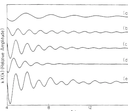
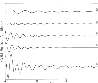
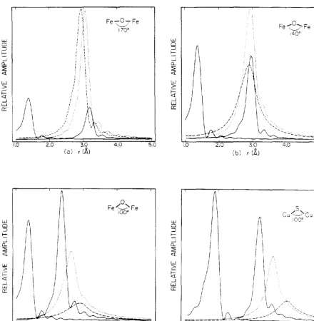
The calculated contribution of each term to the EXAFS at a particular value of the bridging angle (140°) are shown in Figs. 7 and 8. The relative amplitudes of the various terms may be seen from the Fourier transforms in Fig. 9. No corrections were made for damping at large r due to

inelastic scattering, but any such correction would affect the three terms involving the second-shell atom almost equally (the first shell peak would be relatively higher, however). Compared to the second-shell single scattering term, multiple scattering is significant in systems in which the ratio of the scattering power of the first- and second-shell-nearest neighbors is large or when the three atoms are nearly colinear.

30

manner, and hence the effect on the Fourier transform is

similar to that of a Debye-Waller factor.

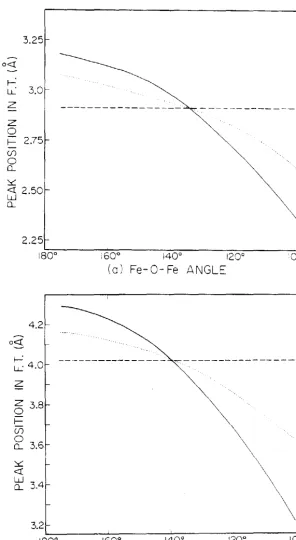
Figures 10 and 11 show the variations of the peak

positions and amplitudes in the Fourier transform as a

function of bridging angle for both the iron and copper

systems. Note that, in Figs. lO(a) and lO(b), there is a

point where the additional phase shift incurred during the

multiple scattering process is exactly offset by the

additional path length involved in that process. This

occurs because, the effect of the scattering phases in the

sine argument of Eq. (2.4.17), is to shift the peaks in

the Fourier transform to smaller distances, since these

phase are largely monotonically decreasing functions of k.26

The condition required for this crossover point is

given by:

l r · l - l r · l - l r · - r·l

= ilr("'·)

1 J 1 J "'J (2.5.1)

where 6r(¢jl is the effective displacement of the peak in

the Fourier transform due to the phase of the scattering

amplitude associated with atom j. This quantity, 6r(tl>j), is

independent of the geometry of the system (provided the

phase of the scattering amplitude is independent of the

scattering angle, as discussed earliel:}, and varies over a

limited range for different atom types j. The primary

dependence of the crossover point is on the bond lengths; as

the distances in the system increase, the crossover point

occurs at larger bridging angles.

31

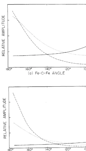
the multiple scattering terms are of particular importance.

As shown in Fig. 11 these terms have large amplitudes at

high angles and, above the crossover point, the

corresponding peaks in the Fourier transform occur at

smaller distance values than does the second-shell single

scattering peak. In general, the three peaks involving the

second-shell atom will be close enough to overlap in the

transform. The presence of the multiple scattering

components will then cause an apparent increase in the

amplitude of the second-nearest neighbor peak in addition to

shifting this peak to anomalously small distances.

Therefore, if an analysis of EXAFS data which contain a

significant multiple scattering contribution, is attempted

using single scattering theory, one would overestimate the

coordination number of the second-shell and underestimate

the distance to that shell. Recently, Co et al.2 7 studied a

series of ~-oxo bridged iron system~ using single scattering

theory, their results are shown in Fig. 12. For a linear

system, Co et al. predict an error in the coordination

number of a factor of four and an underestimation of the

distance by 0.2 ~. These results may be compared directly

with the calculations for the ~-oxo system shown in Figs.

lO(a) and ll(a). Since, when the system is linear, both

multiple scattering components have comparable amplitudes

and clearly dominate the second-shell EXAFS, the position of

the composite second-shell peak may be taken as the average

32

Therefore, we calculate from Fig. lO(a) that the average of the multiple scattering peak positions is smaller than that of second-shell single scattering peak by an amount of 0.21

~. This is in excellent agreement with the observations of Co et al. A similar analysis when applied to the peak amplitudes in Fig. ll(a) yields an overestimation of the second-shell coordination number by a factor of eight. The calculated peak amplitudes are clearly inconsistent with the experimental observations. 27 The origin of this discrepancy is the omission of both the Debye-Waller and inelastic damping factors from the theoretical calculations. Chapters IV and V present a detailed study of the nature of the Debye-Waller factors in EXAFS.

At bridging angles which are smaller than the crossover po in t, the compos i t e second-she 11 . peak w i 11 occur at a larger distance than the second-shell single scattering peak; the effect is less significant, however, since the multiple scattering components have smaller amplitudes in this reg ion.

33

Appendix A

We wish to evaluate the integral

I

=

J<k

I

r)

e .

r(r

I

i) dr (Al)

which appears in Eq. (3. 1); where (r I k)

=

(217)"312 x exp(ik · r) and (r I i) = (1T)"112(~a

0

)312 exp(-Zr/ a_0).

Expanding Eq. (Al) in terms of spherical harmonics,

I may be rewritten as

xexp(-Zr/a0)r2dr

jY~'"(Q-)Y

1

(Qr)(r·

e)dP.,,

(A2) where dr

=

r2 dr dQr.

The angular integration in Eq. (A2) may be performed using the additional theorem for spherical harmonics:

I2

L

f

y

~'"(Q~)Y'J'(P.r)(r.

e) dQ,

I '"

.,. I 1

= 4;r;;=]; { ;

Yf(P..)Y~'"(n~>jYr'<nr)Y'I'(P.r)dP.,

1

= 4

;r

L

Yf(n.)fi''"(Q~)o,,,o

1

,

1

=

r(k ·

e) • (A3)

, ... 1

Substituting Eq. (A3) into Eq. (A2), the expression for I becomes

I=(21T)-3'24(1T)112(-i)(!}'z<k. e)

x

J-

j₁(kr) exp(-Zr/a₀)yl dr ,

0

(A4)

where it(kr)

=

(kr)"2 sin kr- (kr)"1 cos kr. Making use of the definite integral,

1•

x" e·•n dx

=

nl iJ.-!n•!> , Re iJ. > 0

0

the radial integration in Eq. (A4) may be performed to obtain

I=M(k,Z)(k· e),

34

Appendix B

In this appendix, the angular integrals in Eq. (3.16), (3.17), and (3.19) are evaluated.

The first of these corresponds to 1.1. _0, the hypothetical absorption coefficient in the absence of neighboring atoms. Placing

e

along the z direction:

l.l.oa: :rrfiMI

2

_k·

ednk

Lwlzj

2 •

'I

<

12

=~ cos BksmBkdBkd<b•=3 M k,Z) . The following result is required in Eq. (3. 1 7):

l=J<e·

k)exp(-ik· r₁

lf(B

₁

)'!!&.

(e ·

k)

may be expanded in spherical harmonics, and setting

r

1 along the

z

axis, the azimuthal integration

yields them =0 component in the expansion. Hence:

1=-(e·

t)iJd(cosB,)cosB.exp(-ik· r₁)f(B_{1) ,} (B1) where cosB.=(k· ;). exp(-ik· r₁₎ and/(8₁₎ may be ex-pressed in terms of Legendre polynomials:

exp(-ik· r₁)=L(21+1)(-i)1j₁(kr₁)P1(cos8k), (B2)

I

f(B ₁)

=

L f

,.

₁.P,.(cos Bk) , (B3)

and

(B4)

Substituting the above into Eq. (B1) yields

~ ~ ~ t . I (

47T )1/2 ( 47T )I/2(47T)I/2

l=fr,(e·r1h(21+1)(-t) ₂₁+ _{1 21},+₁

3

xj,(kr₁

)J,.j

Y~.(nk)Yf(n.)Y~(n,)d(-

cosek), (B5) where

an,

=d(- cos8,)d¢_, and

g•

(d¢,/2rr) = 1. The angular integral in Eq. (B5) may be evaluated using the properties of Clebsch- Gordan coefficients24:

J

Y~. (nk)Y~(n,)Y~(n,)

lin.

[(21'+1) 3 ]

1

'2 1 , 2

35

where ll-l'l :Sl:Sil+l'l and l+l'+1=2n (nan inte-ger). The summation over land l' may be replaced by a single sum that has two components l ± 1. Using the explicit forms of the Clebsch-Gordan coefficients above,

1

=

~

(e •

7)!

1

[<-

i)1•1

(;t+

\)il•1(kr1)

+(-1)1-1~l~

₁

)il-t(krJ)] =~(e•

r

1

}fr[:2l!₁ jl-t(kr1)

( l+l). (

)~(

•)1-1

- 21+1 Jl•tkrJ~ -z . (B6)

Using the asymptotic form of the spherical Bessel func-tion:

I= (e ·

r

₁) -1-h[exp(ikr;lf(lT)

+

exp(- ikr,)f(O)] .

kr, .

Hence:

J2 Re[M"'(k •

e)(3. 12)]

~~/

=

-l:

\M \2

k~

(e · ri

Im(exp(2ikr1)/(1T)

+

f(O)] .

J J

The third angular integration necessary is given in Eq. (3.19):

(B7) where fc( 1T -

e

J)

= (-

1)1

/c(e ,)

=

L

i: (-

~)

1 (41T)[exp(2i1i1) -l]i'';'(nk)Y ;"'(nr1 ) •

I m•·l 2zk

Expanding (e •

k)

in spherical harmonics:

1

(e·

~>=

41T

L:

Yf'(n.)Y~,..(nk).

3 m" •-1

Equation (B7) may be written:

I 1

I'= (-

~)

1

41T

L L L

[exp(2i1i_{1) -} l]Y ;"'(nr,)Yj' (n,)

2zk 3 1 m•-1 m'•-1

due to the orthogonality of spherical harmonics. Hence:

!2

Re[M"'(k,

Z)(e • k)(3. 13)]

~a

"<e · r )

2

} =-

\M

j2 L.. / Im{[exp(2i1i₁₎ -1]/1(1T) exp(2ikr1) ,

36

References

*This chapter is based on: J.J. Boland, S.E. Crane and J.D. Baldeschwieler, J. Chern. Phys. 77, 142 (1982).

1. R. de L. Kronig,

z.

Phys. 80, 317 (1931); 75, 191

(1932); 75, 468 (1932).

2. H. Petersen,

z.

Phys. 80, 258 (1933).

3. A.I. Kosterev, Zh. Eksp. Teor. Fiz. 19, 413 (1949).

4. T. Shiraiwa, T. Ishimura and M. Sawada, J. Phys. Soc. Jpn. 138, 848 (1958).

5. D.E. Sayers, F.W. Lytle and E.A. Stern, Adv. x-ray Anal. 13, 248 ( 1970) •

6. W.L. Schaich, Phys. Rev. 8 8, 4028 (1973).

7. E.A. Stern, Phys. Rev. 8 10, 3027 (1974).

8 • C • A. As h 1 e y and S • Do n i a c h , Ph y s • Rev • 8 11 , 1 2 7 9 ( 1975).

9. P.A. Lee and J.B. Pendry, Phys. Rev. 8 11, 2795 (1975).

10. P.A. Lee, Phys. Rev. 8 13, 5261 (1976).

11. P.A. Lee and G. Beni, Phys. Rev. 8 15, 2862 (1977).

37

13. · E.A. Stern, Contemp. Phys. 18, 289 (1978).

14. L.V. Azaroff, Rev. Mod. Phys. 35, 1012 (1963).

15. V.V. Schmidt, Bull. Acad. Sci. USSR, Ser. Phys. 25, 988 (1961).

16. E. Merzbacher, Quantum Mechanics, 2nd ed. (Wiley, New York) p. 466.

17. J.R. Taylor, Scattering Theory (Wiley, New York, 1972)

p. 16 8.

18. P. Lloyd and P.V. Smith, Adv. Phys. 21, 69 (1972).

19. L.I. Schiff, Quantum Mechanics, 3rd ed. (McGraw-Hill, New York, 1968) 1 p. 338.

20. M. Lax, Rev. Mod. Phys.

23,

287 (1951).

21. J.R. Taylor, Ref. 19, p. 43.

22. J.R. Taylor, Ref. 19, p. 54.

23. B.K. Teo, P.A. Lee, A.L. Simons, P. Eisenberger and B.M. Kincaid, J. Am. C.hem. Soc. 99, 3854 (1977).

24. E. Merzbacher, Ref. 16, p. 396.

38

26. P.A. Lee, B.K. Teo and A.L. Simons, J. Am. Chern. Soc. 99, 3856 (1977).

27. M.S. Co, W.A. Hendrickson, K.O. Hodgson and S. Doniach

J. Am. Chern. Soc. 105, 1144 (1983).

28. B.K. Teo, J. Am. Chern. Soc. 103, 3990 (1981).

29. J.J. Barton,

c.c.

Bahr,

z.

Hussain,

s.w.

Robey, J.G. Tobin, L.E. Klebanoff and D.A. Shirley, Phys. Rev.

39

Figure 1.

[image:51.547.57.467.113.599.2]

i I I I i I

0

'·)

0

'·a r

~

r

+ +

\L

+ + + +

~

c c c c

t~ G+

I 0

t7

G;

t•G•t:'"G+ c 0 J 0 (G~tT G~ t• G+ t•G+ I 0 J 0 t•G+ t•G+ J 0 I 0

Figure 2.

Diagrammatic representation of the first and second order terms in the expansion of the full T operator in Eq.

(2.2.6). The scattering paths shown are those that occur in

41

Figure 3.

[image:53.547.212.275.172.463.2]

Figure 4.

42

I

I

I

A

I

I

[image:54.548.140.387.103.471.2]

43

lo I lo

'·,Q

r

...-\

lc

lo

)

1\L

c)

~

c

a, r;

G;

lbl t~ G~ C) t+G+ _{c 0} t• G+

J 0

'd, t;s;ttG;

e: t•G• t• G•

' I 0 J :J

I I I I I

'9

Q

Q

_c

'@

_c

£

f' t• G ... t'• G+ t•G• t•G• t; G"" t• G+ f+G+ t•G• + + + + + + _{t• G• tG+ r:G• t:'"G•}

!g) hi 1, t

1 G0 t1 G0 t1 G0 I

I j Q I Q C 0 I 0 I 0 C Q j Q I Q C O J O I O J O

Figure 5.

The most significant scattering paths within the three-atom system. The operators shown with eaco diagram represent the corresponding term in the exp9nsion of the full T operator in the Lippmann-Schwinger equation [Eq.

44

I~

c•

(a )

(b)

(c)

(d)

Figure 6.

Schematic representation of the terms in the EXAFS

expression for the three-atom system. Note that no

scattering is shown by the central atom since the spherical

Q_

E

<!

Q)

>

0

Q)

0:::

><

..OS:.

45

I

-

- - - -

(a)

( b) I

( c )

(d)

(e)

4

8

12

16

Figure 7.

[image:57.557.51.466.109.466.2]

46

(a)

(b) Q.)

-o

:J

-

Q_

E

(c)

<r

Q.) >

-

0 (d)

Q.)

a:

.cL

><

.cL

4

Figure 8.

[image:58.547.47.461.107.460.2]

47 Fe-0-Fe Fe~':-Fe "--'' 170" 140°

w.J w.J

0 0

::J ::J

I- _f:::

...J ...J

\

~\'

CL CL

:::E ::;;:

<l: <l:

w.J w

> >

I- ~

<l:

/ I \\

...J

j\

...J

w w

a: a: I' \

' ' '

\

1.0 2.0 3.0 4.0 5.0 1.0 2.0 3.0 4.0 5.0

(a) r (A) _{(b) r (A,)}

~

0

FeC'Fe

_/s,

100" _{Cu '-___./ Cu}

w.J

1\

w _II 100c

0 0

::J

I

I

::J

I

I

f:::

I-...J

I

I

...J

I

I

CL CL

::;;:

I

I

:::E

<l:

I

I

<l:

I

I .

w.J

I

I

w

I

I .

2: >

I-I

~

i=

I

I

I

<(

/

<l:

...J

...J _w

w

I

0:: I

I .

a:

I

)

I

/ .·

\~n//',,

__

I /

~

//~

.. ,.. ... ...,-'""""""'"""''""''' ... ~---- ' . .,.,.,_~

1.0 4.0 5.0 1.0 2.0 3.0 4.J 5.0

(c)

_:d:'

_r (A)

Figure 9.

[image:59.548.35.475.72.521.2]

o<t:

r-:

LL z

z

0

f---U) 0

o_

:::.::::

i'5

2.50 o_

o<(

z

z

0

f---U) 0

o_

:::.::::

<(

w

0..

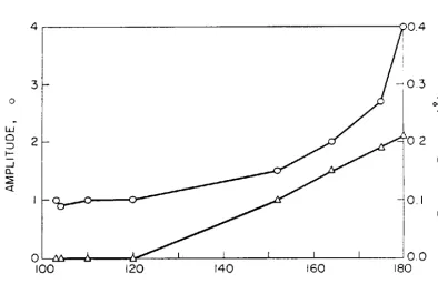
Figure 10.

48

i60° 140° 120° (a) Fe-0-Fe ANGL::

160° 140° 120° (b) Cu-S-Cu ANGLE

Peak positions in the Fourier transform as a function of bridging angle. The solid curve is the second shell single scattering, while the dotted and dashed curves are the double and triple scattering pathways. (a) Fe system.

[image:60.553.84.380.50.590.2]