Volume 2010, Article ID 191085,7pages doi:10.1155/2010/191085
Research Article
Eigenvectors of the Discrete Fourier Transform Based on
the Bilinear Transform
Ahmet Serbes and Lutfiye Durak-Ata (EURASIP Member)
Department of Electronics and Communications Engineering, Yildiz Technical University, Yildiz, Besiktas, 34349, Istanbul, Turkey
Correspondence should be addressed to Ahmet Serbes,[email protected]
Received 19 February 2010; Accepted 24 June 2010
Academic Editor: L. F. Chaparro
Copyright © 2010 A. Serbes and L. Durak-Ata. This is an open access article distributed under the Creative Commons Attribution License, which permits unrestricted use, distribution, and reproduction in any medium, provided the original work is properly cited.
Determining orthonormal eigenvectors of the DFT matrix, which is closer to the samples of Hermite-Gaussian functions, is crucial in the definition of the discrete fractional Fourier transform. In this work, we disclose eigenvectors of the DFT matrix inspired by the ideas behind bilinear transform. The bilinear transform maps the analog space to the discrete sample space. Asjωin the analogs-domain is mapped to the unit circle one-to-one without aliasing in the discretez-domain, it is appropriate to use it in the discretization of the eigenfunctions of the Fourier transform. We obtain Hermite-Gaussian-like eigenvectors of the DFT matrix. For this purpose we propose three different methods and analyze their stability conditions. These methods include better conditioned commuting matrices and higher order methods. We confirm the results with extensive simulations.
1. Introduction
Discretization of the fractional Fourier transform (FrFT) is vital in many application areas including signal and image processing, filtering, sampling, and time-frequency analysis [1–3]. As FrFT is related to the Wigner distribution [1], it is a powerful tool for time-frequency analysis, for example, chirp rate estimation [4].
There have been numerous discrete fractional Fourier transform (DFrFT) definitions [5–11]. Santhanam and McClellan [5] define a DFrFT simply as a linear combination of powers of the DFT matrix. However, this definition is not satisfactory, since it does do not mimic the properties of the continuous FrFT.
Candan et al. [6] use the S matrix, which has been introduced earlier by Dickinson and Steiglitz [12] to find the eigenvectors of the DFT matrix in order to generate a DFrFT matrix. The S matrix commutes with the DFT matrix, which ensures that both of these matrices share at least one eigenvector set in common. This approach is based on the second-order Hermite-Gaussian generating differential equation. Candan et al. [6] simply replace the derivative operator with the second-order discrete Taylor
approximation to second derivative and the Fourier operator with the DFT matrix.
Pei et al. [7] define a commutingTmatrix inspired by the work of Gr¨unbaum [13], whose eigenvectors approximate the samples of continuous Hermite-Gaussian functions better than the eigenvectors ofS. Furthermore, the authors use linear combinations ofS and Tmatrices as S+kT to furnish the basis of eigenvectors for the DFrFT matrix.
Candan introduces Sk [8] matrices whose eigenvectors are higher-order approximations to the Hermite-Gaussian functions. The idea is to employ higher-order Taylor series approximations to the derivative operator, which replaces the second derivative operator in the Hermite-Gaussian generating differential equation. However, the order of approximationkis limited by the dimension of theSkmatrix 2k+ 1≤N.
Pei et al. [10] recently removed the upper bound of this approximation and obtained higher—order approximations. However, it needs high computational cost to generate Pei’s Sk matrices. More recently, in [14] the authors present the closed form ofSkmatrix ask → ∞in the limit.
as its bilinear discrete equivalent to discretize the Hermite-Gaussian differential equation. Since the bilinear transform maps the analog domain to the discrete domain one-to-one, we find eigenvectors which are close to the samples of the Hermite-Gaussian functions. We also analyze the stability issues. Additionally, two more methods are proposed, which employ better conditioned and higher-order bilinear matrices.
The paper is organized as follows. Section 2 gives introductory information on Hermite-Gaussian functions, basics of how to generate commuting matrices and the bilinear transform. Section 3presents the proposed meth-ods by defining the bilinear transform-based commuting matrices including the stability analysis. Simulation results and performance analysis are given inSection 4. The paper concludes inSection 5.
2. Preliminaries
2.1. Hermite-Gaussian Functions. The Hermite-Gaussian functions span the space of Hilbert space L2(R) of square
integrable functions, which are well localized in both time and frequency domains. These functions are defined by a Hermite polynomial modulated with a Gaussian function
Ψm(t)=√21/4 2mm!Hm
√
2πte−πt2, (1)
whereHm(t) is themth-order Hermite polynomial. Hermite-Gaussian functions are eigenfunctions of the Fourier trans-form
F{Ψm}(t)=e−jmπ/2Ψm(t), (2)
where F is the Fourier transformation operator and e−jmπ/2is themth-order eigenvalue. Anmth-order
Hermite-Gaussian function has m zero-crossings. The Hermite-Gaussian functions are homogeneous solutions of the dif-ferential equation, which is also known as the Hermite-Gaussian generating differential equation
d2f(t) dt2 −4π
2t2f(t)=λ f(t), (3)
withλ=2m+ 1. The Hermite-Gaussian generating function can be expressed by its operator equivalent as
D2+F D2F−1f(t)=λ f(t), (4)
whereD2denotes the second derivative operator.
2.2. Commuting Matrix Generation. LetAandBbeN×N square matrices. IfAB=BA, thenAandBare commuting matrices. IfAandBcommute, they share at least one set of common eigenvector sets [6].
Candan [8] showed that a DFT commuting matrixKcan be obtained for any arbitraryN×NmatrixLas
K=L+FLF−1+F2LF−2+F3LF−3, (5)
whereFis theNpoint DFT matrix which is defined as
(F)n,m= 1 √
Nexp
−j2π
Nnm
, n,m=0, 1,. . .,N−1.
(6)
In [10] it is shown that if L commutes with F2, (5) is
simplified to
K=L+FLF−1. (7)
Theorem 1. One can further extend this idea such that, ifLis circulant and symmetric the above equation is also valid.
Proof. LetCbe a circulant and symmetric matrix, then the eigenvalue decomposition ofCis [15, pages 201-202]
C=F−1ΛCF, (8)
where ΛC = diag( √
NFc) is a diagonal matrix containing eigenvalues ofC. Here,cis the first column ofC,andN is the dimensional ofC. AsCis symmetric, the above equation is equivalent to
C=FΛCF−1 (9)
since the symmetry implies that CT = C. Hence we can conclude that C+FCF−1 = F2CF−2 +F3CF−3 when we
replace (9) in the left hand side and (8) in the right hand side of this equation. Consequently, the proof of
K=C+FCF−1 (10)
is complete. We can conclude that while generating DFT commuting matrices, a good choice is to chose real, symmetric and circulant matrices and replace them withC in (10).
2.3. Bilinear Transform. Bilinear transform is a useful and popular tool in signal and system analysis, which is often used to map the Laplaces-domain to thez-domain. There are numerous finite difference approximation (FDA) methods for this mapping. The most popular ones are the forward and backward difference methods and the bilinear transform. The forward difference method discretizes the derivative operator by mapping dx(t)/dt⇒(x(n)−x(n−1))/Δtwhereas the backward difference method impose dx(t)/dt ⇒(x(n+ 1)−x(n))/Δt.
The bilinear transform defines the discrete differentiation of a signalx(n) as
x(n) +x(n−1)= c
Δt(x(n)−x(n−1)), (11)
wherex(n) is the discrete derivative ofx(n),Δt =1/√Nis the sampling period,Nis the length of the signalx(n), and cis a real scalar. Hence, the second-order discrete derivative x(n) can be defined through the centered form expression
x(n−1) + 2x(n) +x(n+ 1)
=
c
Δt 2
The bilinear transform maps the analog domain to the discrete domain one-to-one. It maps points in thes-domain with Re{s} = 0 (jω axis) to the unit circle in the z-plane |z| = 1. However, the forward difference method maps the jωto a circle of radius 0.5 and centered at the pointz=0.5 as shown inFigure 1. Bilinear transform maps every point in thejω-plane to thez-plane without aliasing.
We express (12) in matrix form as
B1X=
c
Δt 2
E2X, (13)
where X = [x(0),x(1),. . .,x(N − 1)]T, X =
[x(0),x(1),. . .,x(N−1)]T with
B1= ⎡ ⎢ ⎢ ⎢ ⎢ ⎢ ⎢ ⎢ ⎢ ⎢ ⎢ ⎢ ⎢ ⎢ ⎢ ⎢ ⎢ ⎣
2 1 0 · · · 0 1
1 2 1 · · · 0
0 1 2 . .. ... ..
. . .. ... ... ...
..
. . .. ... 1
1 0 0 · · · 1 2
⎤ ⎥ ⎥ ⎥ ⎥ ⎥ ⎥ ⎥ ⎥ ⎥ ⎥ ⎥ ⎥ ⎥ ⎥ ⎥ ⎥ ⎦ , (14)
E2= ⎡ ⎢ ⎢ ⎢ ⎢ ⎢ ⎢ ⎢ ⎢ ⎢ ⎢ ⎢ ⎢ ⎢ ⎢ ⎢ ⎢ ⎣
−2 1 0 · · · 0 1
1 −2 1 · · · 0
0 1 −2 . .. ...
..
. . .. ... ... ...
..
. . .. ... 1
1 0 0 · · · 1 −2
⎤ ⎥ ⎥ ⎥ ⎥ ⎥ ⎥ ⎥ ⎥ ⎥ ⎥ ⎥ ⎥ ⎥ ⎥ ⎥ ⎥ ⎦ . (15)
Hence, we conclude with an equivalent form of discrete second derivative as
X=
c
Δt 2
B−1
1 E2X, (16)
with the discrete second derivative operator D2 =
(c/Δt)2B−1 1 E2.
3. Obtaining DFT Commuting Matrices
An easy and accurate way of obtaining Hermite-Gaussian-like eigenvectors of the DFT matrix is to define a better commuting matrix, which imitates the Hermite-Gaussian generating differential equation given in (3) as a discrete substitute. In this section we disclose an elegant way of obtaining better commuting matrices by taking advantage of the bilinear transform, which is a good discrete substitute for the derivative operator.
The algorithm is straightforward; we substitute the second derivative and the Fourier transform operators in (3) with the matrix given in (16) and the DFT matrix,
−1 −0.8 −0.6 −0.4 −0.2 0 0.2 0.4 0.6 0.8 1
−1 −0.8 −0.6 −0.4 −0.2 0 0.2 0.4 0.6 0.8 1 Real{z}
Figure1: Image ofjωaxis in thez-plane for bilinear transform and the forward difference method. Solid: bilinear transform, dashed: forward difference method.
respectively. Hence, DFT commuting matrix inspired by the bilinear transform is given by
B=B−1
1 E2+FB−11E2F−1. (17)
We omit the coefficient (c/Δt)2, since it has no effect on the eigenvectors ofB.
Theorem 2. Bcommutes with the DFT matrix.
Proof. AsB1andE2are both circulant and symmetric,B−11E2
is symmetric and circulant also. We useTheorem 1given in
Section 2.2, which states thatany circulant and symmetric matrixCcan be used to generate a commuting matrix as in (10). SinceB−11E2is both circulant and symmetric, the proof
is complete.
After generating the commuting matrix B, we find its eigenvectors. The eigenvectors are Hermite-Gaussian-like eigenvectors with the number of zero-crossings equal to the order of Hermite-Gaussian eigenvectors. InSection 4we give extensive simulations and results on these Hermite-Gaussian like eigenvectors.
3.1. Stability. Stability of B can easily be proved when B1 is not singular. We can show this by the eigenvalue
decomposition ofB1
B1=F−1ΛB1F, (18)
is the dimension ofΛB1. Asb1 = [2, 1, 0, 0,. . ., 1] T
, Fourier transform ofb1can be easily found and replaced to find the
eigenvaluesΛB1
ΛB1=diag
2 + 2 cos
2πn N
, n=0, 1, 2,. . .,N−1.
(19)
ΛB1is never zero for oddN, since diag(2 + 2 cos(2πn/N))> 0 for all n. However as N increases ΛB1 becomes poorly conditioned. Besides, for evenN, diag(2 + 2 cos(2πn/N))=0 forn = N/2, which causes instability. We can add a small
ξ >0 in the diagonal ofB1to overcome instability. ThenΛB1
is changed to
ΛB1=diag
2 +ξ+ 2 cos
2πn N
, n=0, 1, 2,. . .,N−1
(20)
to preserve stability for even N. Consequently, to ensure stability we substituteB1defined in (14) with
B1= ⎡ ⎢ ⎢ ⎢ ⎢ ⎢ ⎢ ⎢ ⎢ ⎢ ⎢ ⎢ ⎣
2 +ξ 1 0 · · · 0 1
1 2 +ξ 1 · · · 0
0 1 2 +ξ . .. ...
..
. . .. ... ... ...
..
. . .. ... 1
1 0 0 · · · 1 2 +ξ
⎤ ⎥ ⎥ ⎥ ⎥ ⎥ ⎥ ⎥ ⎥ ⎥ ⎥ ⎥ ⎦ . (21)
Adding a smallξ value in the diagonal will not perturb the eigenvectors of the commuting matrix.
3.2. Better Conditioned Bilinear Methods. Bilinear transform can be considered as a trapezoidal approach to the derivative. Hence, we can assure stability by using alternative B1
matrices. We have found out that changing the diagonal ofB1 by a constant k > 2 both ensures the stability and
increases the performance. Therefore we substituteB1with
B1, where we defineB1as
B1= ⎡ ⎢ ⎢ ⎢ ⎢ ⎢ ⎢ ⎢ ⎢ ⎢ ⎢ ⎢ ⎣
k 1 0 · · · 0 1
1 k 1 · · · 0
0 1 k . .. ... ..
. . .. ... ... ... ..
. . .. ... 1
1 0 0 · · · 1 k
⎤ ⎥ ⎥ ⎥ ⎥ ⎥ ⎥ ⎥ ⎥ ⎥ ⎥ ⎥ ⎦ . (22)
Ask > 2, the commuting matrix is better conditioned. The
optimum value ofkis found to be approximately 4.3, which is given inSection 4.
3.3. Higher-order Bilinear Differentiation Matrix Substitutes.
So far, we have used the bilinear—transform—inspired matrices to find a better discrete substitute for the sec-ond derivative. To find better definitions of differentiation matrices we suggest that a Taylor series-like approach toB1
Table1: Optimumaicoefficients generated forB14.
ai Optimum Value
a1 1.00
a2 0.247634068038315
a3 −0.103839534211561
a4 −0.141176982675410
a5 0.005956945393076
a6 −0.008133047918379
a7 −0.020103743248487
a8 −0.001866823892062
a9 −0.000336065416294
a10 −0.002383849560258
a11 −0.000725049220057
a12 −0.000698349278537
a13 −0.003339855815284
a14 −0.001759635742928
(1) Compute one ofB1 ,B1, orBnmatrices.
(2) Replace the computed matrix in (17) as a substitute for
B1and compute the DFT-commuting matrixB. (3) Find the eigenvectors ofB, which are
Hermite-Gaussian-like orthonormal vectors.
Algorithm1: Summary of the proposed algorithms.
will grant us higher-order bilinear differentiation matrices. Therefore, we define higher-order bilinear differentiation matrices as
Bn=a1B1+a2
B1 2
+· · ·+an
B1 n
, (23)
where we nameBn asnth-order bilinear approximation to the second derivative, andaiare real scalars. The value ofk= 4.3 is chosen forBn, as it is an optimum value with respect to minimum total error norm which is discussed inSection 4. We have not come up with an analytical expression ofai’s yet, however, genetic and/or pattern search algorithms may be used to optimize the coefficients.
We have used the genetic [16] and the pattern search [17] algorithms and determined optimum ai coefficients, i=1, 2,. . ., 14, which are given inTable 1. These coefficients are inserted in (23) to obtain B14. We have generated the
commuting matrix B by substituting B1 withB14 in (17).
When B14 is employed, eigenvectors ofB are found to be
very close to the samples of Hermite-Gaussian functions as the performance is discussed in detail in the verySection 4.
So far, three different methods are proposed, which are summarized in Algorithm 1. The first method computes
B1, in which a small ξ is added in the diagonal ofB1
to achieve stability. In the second method we alter the diagonal ofB1, with a value k > 2. Changing the diagonal
both improves the performance and ensures stability. In the last proposed method we find higher-order matrices, using the B1 and its weighted powers with k = 4.3
for a better definition of the commuting matrix. After-wards, we replace the computed B1, B1, or Bn with B1
5 10 15 20 25 30 35 40 45 50 55
2 3 4 5 6 7 8 9 10
(k)
T
o
tal
n
or
m
o
f
er
ror
N=64 N=56
N=48 N=40 N=32
(a)
10−2
10−1
100
0 5 10 15 20 25 30
Number of zero crossing
log
10
(nor
m
o
f
er
ror)
B1,k=2 +ξ B1,k=3
B1,k=4 B1,k=4.3
(b)
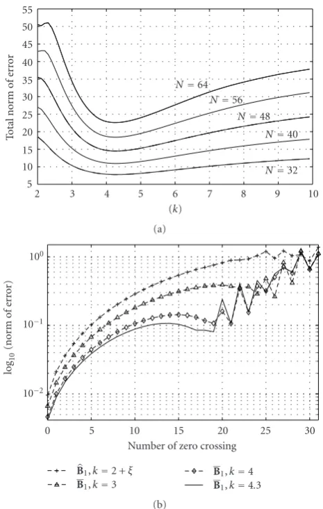
Figure2: (a) The total norm of error versuskinB1forN =32, 40, 48, 56, andk=4.3. The total norm of error is minimum when
k ≈4.3. (b) Error norms between the discrete Hermite-Gaussian like eigenvectors and the samples of the Hermite-Gaussian functions whenB1fork=3, 4, andk=4.3 andB1 withN=32.
matrix whose eigenvectors are the Hermite-Gaussian-like orthonormal vectors.
4. Simulations and Results
We have proposed three different techniques for finding Hermite-Gaussian-like eigenvectors of the DFT. In the first method we employB1defined in (21). As a second method
we useB1as defined in (22) for different values ofk. Finally,
we employ Bn given in (23). We replace each matrices in (17) as a substitute toB1to generate commuting matricesB.
Afterwards, we find eigenvectors of these commuting matri-ces and find the norm of error between samples of corre-sponding Hermite-Gaussian functions and the eigenvectors. First we compare total norms of errors between the Gaussian functions and the samples of Hermite-Gaussian-like eigenvectors to determine optimumkforB1.
We define the total norm of error as sum of norms of error for each eigenvector.Figure 2(a)shows the total norm of error
10−6
10−5
10−4
10−3
10−2
10−1
100
0 5 10 15 20 25 30
Number of zero crossings
log
10
(nor
m
o
f
er
ror)
B1 S2
S6 S16
(a)
10−8
10−7
10−6
10−5
10−4
10−3
10−2
10−1
100
0 10 20 30 40 50 60
Number of zero crossings
log
10
(nor
m
o
f
er
ror)
B1 S2
S6 S16
(b)
Figure3: Error norms between the discrete Hermite-Gaussian like eigenvectors and the samples of the Hermite-Gaussian functions of
B1method whenk=4.3 are compared with various other methods for (a)N=32 and (b)N=64.
versuskfor different values ofN, and the best value forkis approximately 4.3.
Comparison of errors betweenB1fork =3, 4, and 4.3
andB1with the dimensionalN=32 is given inFigure 2(b).
The error norm is measured as the norm of error between the samples of Gaussian functions and Hermite-Gaussian like eigenvectors of B using these matrices. As it is clear from the figures, the best overall performance is obtained in theB1method whenk=4.3.
Figure 3(a) plots the norms of errors for different methods defined in [8]. We compare the error norms of S2,S6, andS16 in between, which are ofO(h2),O(h6), and O(h16) Taylor approximations, respectively, as shown in [8],
0 0.2 0.4 0.6 0.8 1 1.2 1.4
0 5 10 15 20 25 30 35
Number of zero crossings
No
rm
o
f
er
ro
r
B14 S100
S400 S32
Figure 4: Comparison of error norms between the discrete
Hermite-Gaussian like eigenvectors and the samples of the Hermite-Gaussian functions ofB14andS32,S100, andS400methods forN=32.
the same comparison forN = 64. These plots show that our proposed algorithm is slightly worse than some other methods for small orders, but much better for higher-orders of eigenvectors. As it is clear from the figures, our method outperforms the other methods in total.
We compare the proposed higher-order B14 method
with the other higher-order methods, S32, S100, and S400
that employ higher-order Taylor approximations to the second derivative as shown in [10]. Figure 4 presents the performance of the proposed method together with the other methods. Despite the fact that our method uses only the 14th order approximation, it is definitely better than these methods, even better thanS400.
5. Conclusions
As the eigenvectors that are closer to the samples of continuous Hermite-Gaussian functions are important for a better definition of DFrFT, we employ bilinear transform-based methods to define better commuting matrices. We have proposed three different methods and analyzed their stability issues. A stable method is proposed by inserting a small ξ in the diagonal of the bilinear matrix. Better— conditioned bilinear differentiation matrices that have better performance are also obtained. Besides, a method of generating higher-order bilinear differentiating matrices is also suggested.
Simulation results show that the proposed methods posess better eigenvectors when compared to the other methods recently suggested.
Future works on this subject may include finding a closed form expression for the coefficients generating the higher-order bilinear matrices,Bn. Furthermore,Bnmatrices
may be used in linear combinations with other commuting matrices, such asS2k.
References
[1] H. M. Ozaktas, Z. Zalevski, and M. A. Kutay, The Frac-tional Fourier Transform with Applications in Optics and Signal Processing, John Wiley & Sons, New York, NY, USA, 2001.
[2] M. A. Kutay, H. M. Ozaktas, O. Ankan, and L. Onural, “Optimal filtering in fractional Fourier domains,”IEEE Trans-actions on Signal Processing, vol. 45, no. 5, pp. 1129–1143, 1997.
[3] X.-G. Xia, “On bandlimited signals with fractional Fourier transform,”IEEE Signal Processing Letters, vol. 3, no. 3, pp. 72– 74, 1996.
[4] O. Akay and G. F. Boudreaux-Bartels, “Fractional convolution and correlation via operator methods and an application to detection of linear FM signals,”IEEE Transactions on Signal Processing, vol. 49, no. 5, pp. 979–993, 2001.
[5] B. Santhanam and J. H. McClellan, “The discrete rotational Fourier transform,”IEEE Transactions on Signal Processing, vol. 44, no. 4, pp. 994–998, 1996.
[6] C¸. Candan, M. A. Kutay, and H. M. Ozaktas, “The discrete fractional Fourier transform,” IEEE Transactions on Signal Processing, vol. 48, no. 5, pp. 1329–1337, 2000.
[7] S.-C. Pei, W.-L. Hsue, and J.-J. Ding, “Discrete fractional Fourier transform based on new nearly tridiagonal commut-ing matrices,”IEEE Transactions on Signal Processing, vol. 54, no. 10, pp. 3815–3828, 2006.
[8] C¸. Candan, “On higher order approximations for Hermite-Gaussian functions and discrete fractional Fourier trans-forms,”IEEE Signal Processing Letters, vol. 14, no. 10, pp. 699– 702, 2007.
[9] S.-C. Pei, J.-J. Ding, W.-L. Hsue, and K.-W. Chang, “Gener-alized commuting matrices and their eigenvectors for DFTs, offset DFTs, and other periodic operations,”IEEE Transac-tions on Signal Processing, vol. 56, no. 8, pp. 3891–3904, 2008.
[10] S.-C. Pei, W.-L. Hsue, and J.-J. Ding, “DFT-commuting matrix with arbitrary or infinite order second derivative approximation,”IEEE Transactions on Signal Processing, vol. 57, no. 1, pp. 390–394, 2009.
[11] B. Santhanam and T. S. Santhanam, “Discrete Gauss-Hermite functions and eigenvectors of the centered discrete Fourier transform,” inProceedings of the IEEE International Conference on Acoustics, Speech and Signal Processing ( ICASSP ’07), vol. 3, pp. 1385–1388, 2007.
[12] B. W. Dickinson and K. Steiglitz, “Eigenvectors and functions of the discrete Fourier transform,” IEEE Transactions on Acoustics, Speech, and Signal Processing, vol. 30, no. 1, pp. 25– 31, 1982.
[13] F. A. Gr¨unbaum, “The eigenvectors of the discrete Fourier transform: a version of the Hermite functions,” Journal of Mathematical Analysis and Applications, vol. 88, no. 2, pp. 355– 363, 1982.
[14] A. Serbes and L. Durak, “Efficient computation of DFT commuting matrices by a closed–form infinite order approxi-mation to the second differentiation matrix,”Signal Process. In press.
[16] D. E. Goldberg, Genetic Algorithms in Search, Optimzation and Machine Learning, Addison-Wesley, Reading, Mass, USA, 1989.