Sizes, colour gradients and resolved stellar mass distributions for the massive cluster galaxies in XMMUJ2235 2557 at z = 1 39

Sizes, Colour gradients and Resolved Stellar Mass Distributions for

the Massive Cluster Galaxies in XMMUJ2235-2557 at z = 1.39

Jeffrey C.C. Chan

1

,

2

∗

, Alessandra Beifiori

2

,

1

, J. Trevor Mendel

1

, Roberto P. Saglia

1

,

2

,

Ralf Bender

1

,

2

, Matteo Fossati

2

,

1

, Audrey Galametz

1

, Michael Wegner

2

,

David J. Wilman

2

,

1

, Michele Cappellari

3

, Roger L. Davies

3

, Ryan C. W. Houghton

3

,

Laura J. Prichard

3

, Ian J. Lewis

3

, Ray Sharples

4

and John P. Stott

3

1_{Max-Planck-Institut für extraterrestrische Physik (MPE), Giessenbachstr. 1, D-85748 Garching, Germany} 2_{Universitäts-Sternwarte, Ludwig-Maximilians-Universität, Scheinerstrasse 1, D-81679 München, Germany}

3_{Sub-department of Astrophysics, Department of Physics, University of Oxford, Denys Wilkinson Building, Keble Road, Oxford OX1 3RH, UK} 4_{Centre for Advanced Instrumentation, Department of Physics, Durham University, South Road, Durham DH1 3LE, UK}

Accepted 2100 December 3. Received 2050 December 3; in original form 2014 November 13

ABSTRACT

We analyse the sizes, colour gradients, and resolved stellar mass distributions for 36 massive and passive galaxies in the cluster XMMUJ2235-2557 at z=1.39 using optical and near-infrared Hubble Space Telescope imaging. We derive light-weighted Sérsic fits in five HST bands (i775,z850,Y105,J125,H160), and find that the size decreases by∼20% going fromi775 toH160band, consistent with recent studies. We then generate spatially resolved stellar mass maps using an empirical relationship betweenM∗/LH160 and(z850−H160)and use these to derive mass-weighted Sérsic fits: the mass-weighted sizes are∼41% smaller than their rest-framer-band counterparts compared with an average of∼12% atz∼0. We attribute this evolution to the evolution in theM∗/LH160 and colour gradient. Indeed, as expected, the ratio of mass-weighted to light-weighted size is correlated with the M∗/L gradient, but is also mildly correlated with the mass surface density and mass-weighted size. The colour gradients (∇z−H)are mostly negative, with a median value of∼0.45 mag dex−1, twice the local value. The evolution is caused by an evolution in age gradients along the semi-major axis (a), with

∇age=dlog(age)/dlog(a)∼ −0.33, while the survival of weaker colour gradients in old, local galaxies implies that metallicity gradients are also required, with∇Z=dlog(Z)/dlog(a) ∼ −0.2. This is consistent with recent observational evidence for the inside-out growth of passive galaxies at high redshift, and favours a gradual mass growth mechanism, such as minor mergers.

Key words: galaxies: clusters: general – galaxies: elliptical, lenticular, cD – galaxy: evolution – galaxies: formation – galaxies: high-redshift – galaxies: fundamental parameters.

1 INTRODUCTION

The study of galaxy clusters at high redshift has attracted a lot of attention over the last decade, as these large structures provide a unique environment for understanding the formation and evolution of massive galaxies we see in the present day Universe. Massive galaxies in clusters especially in the cluster cores are preferentially in the red passive population, have regular early-type morphology and are mainly composed of old stars (e.g. Dressler 1980; Rosati et al. 2009; Mei et al. 2009). Nevertheless, in higher redshift clus-ters (z&1.5) a substantial massive population are recently found

∗ E-mail: jchan@mpe.mpg.de

to be still actively forming stars (e.g. Hayashi et al. 2011; Gobat et al. 2013; Strazzullo et al. 2013; Bayliss et al. 2014). The mem-ber passive galaxies reside on a well-defined sequence in colour-magnitude space, namely the red sequence which is seen in clusters up to redshiftz∼2 (e.g. Kodama & Arimoto 1997; Stanford, Eisen-hardt & Dickinson 1998; Gobat et al. 2011; Tanaka et al. 2013; Andreon et al. 2014). Previous works have shown that the stars in these galaxies have formed (and the star formation was quenched) early, the stellar mass is largely assembled beforez∼1 (e.g. Lid-man et al. 2008; Mancone et al. 2010; Strazzullo et al. 2010; Fass-bender et al. 2014). These galaxies then evolve passively in the subsequent time (e.g. Andreon 2008; De Propris, Phillipps & Bre-mer 2013). Nonetheless, the details of how these massive passive

cluster galaxies formed and evolved, in particular the physical pro-cesses involved, remains a matter of debate.

An important component of the above question is the evolu-tion of the structure of these passive galaxies over time. It has now been established that galaxies at high redshift are much more com-pact: those with stellar massesM∗>1011Matz∼2 have an

ef-fective radius of only'1 kpc (e.g. Daddi et al. 2005; Trujillo et al. 2006a). Atz∼0 such massive dense objects are believed to be rel-atively rare (Trujillo et al. 2009), yet the exact abundance is still under debate (Valentinuzzi et al. 2010a; Trujillo, Carrasco & Ferré-Mateu 2012; Poggianti et al. 2013). Previous studies suggest that massive passive galaxies have grown by a factor of∼2 in size since

z∼1 (e.g. Trujillo et al. 2006b; Longhetti et al. 2007; Cimatti et al. 2008; van der Wel et al. 2008; Saglia et al. 2010; Beifiori et al. 2014), and a factor of∼4 sincez∼2 (e.g. Trujillo et al. 2007; Buitrago et al. 2008; van Dokkum et al. 2008; Newman et al. 2012; Szomoru, Franx & van Dokkum 2012; Barro et al. 2013; van der Wel et al. 2014). This progressive growth appears to happen mainly at the outer envelopes, as several works have shown that massive (M∗&1×1011M) passive galaxies at high-redshift have

compa-rable central densities to local ellipticals, suggesting the mass as-semble took place mainly at outer radii over cosmic time (i.e. the “inside-out” growth scenario, Bezanson et al. 2009; van Dokkum et al. 2010; Patel et al. 2013).

To explain the observed evolution, the physical processes in-voked have to result in a large growth in size but not in stellar mass, nor drastic increase in the star formation rate. Most plausible candi-dates are mass-loss driven adiabatic expansion (“puffing-up”) (e.g. Fan et al. 2008, 2010; Ragone-Figueroa & Granato 2011) and dry mergers scenarios (e.g. Bezanson et al. 2009; Naab, Johansson & Ostriker 2009; Trujillo, Ferreras & de La Rosa 2011). In the former scenario, galaxies experience a mass loss from wind driven by ac-tive galactic nuclei (AGN) or supernovae feedback, which lead to an expansion in size due to a change in the gravitational potential. In the latter, mergers either major involving merging with another galaxy of comparable mass, or minor that involves accretion of low mass companions, have to be dry to keep the low star formation rate (Trujillo, Ferreras & de La Rosa 2011). Nevertheless, major merg-ers are not compatible with the observed growth in mass function in clusters as well as the observed major merger rates sincez∼1 (e.g. Nipoti, Londrillo & Ciotti 2003; Bundy et al. 2009). On the other hand, minor mergers are able to produce an efficient size growth (see e.g. Trujillo, Ferreras & de La Rosa 2011; Shankar et al. 2013). The rates of minor mergers are roughly enough to account for the size evolution only up toz.1 Newman et al. (2012), at z∼2 ad-ditional mechanisms are required (e.g. AGN feedback-driven star formation Ishibashi, Fabian & Canning 2013). In addition, the ef-fect of continual quenched galaxies onto the red sequence as well as morphological mixing (known as the “progenitor bias”) further complicates the situation (e.g van Dokkum & Franx 2001). Pro-cesses that are specific in clusters such as harassment, strangula-tion and ram-pressure stripping (e.g. Treu et al. 2003; Moran et al. 2007) might play an important role in quenching and morpholog-ically transforming galaxies. Several studies have already shown that the progenitor bias has a non-negligible effect on the size evo-lution (e.g. Saglia et al. 2010; Valentinuzzi et al. 2010b; Carollo et al. 2013; Poggianti et al. 2013; Beifiori et al. 2014; Delaye et al. 2014; Belli, Newman & Ellis 2015; Shankar et al. 2015).

In addition to size or structural parameter measurements, colour gradients also provide valuable information for disentan-gling the underlying physical processes involved in the evolution of passive galaxies, and have been used as tracers of stellar

popu-lation properties and their radial variation. In local and intermedi-ate redshift passive galaxies, colour gradients are mainly attributed to metallicity gradients (e.g. Saglia et al. 2000; La Barbera et al. 2005; Tortora et al. 2010), although also affected by age and dust (see, e.g. Vulcani et al. 2014). Measuring the colour gradients at high redshift is more challenging due to compact galaxy sizes and limitations on instrumental angular resolution. Passive galaxies at high redshift appear to show negative colour gradients, in the sense that the core is redder than the outskirts (e.g. Wuyts et al. 2010; Guo et al. 2011; Szomoru et al. 2011), implying a radial variation in the stellar mass-to-light ratio (hereafterM∗/L).

Due to M∗/L gradients within the galaxies, the size of the

galaxies measured from surface brightness profiles (i.e. luminosity-weighted sizes) is not always a reliable proxy of the mass distribu-tion, especially at high redshifts when the growth of the passive galaxies is more rapid. Hence, measuring characteristic sizes of the mass distribution (i.e. mass-weighted sizes) is preferable over the wavelength dependent luminosity-weighted sizes. Recently a num-ber of works attempted to reconstruct stellar mass profiles taking into account theM∗/Lgradients primarily using two techniques:

resolved spectral energy distribution (SED) fitting (e.g. Wuyts et al. 2012; Lang et al. 2014) and the use of a scalingM∗/L- colour

rela-tion (e.g. Bell & de Jong 2001; Bell et al. 2003). In the former, stel-lar population modeling is performed on resolved multi-band pho-tometry to infer spatial variations in the stellar population in 2D. While this is a powerful way to derive resolved properties, deep and high-resolution multi-band imaging are required to well con-strain the SED in each resolved region, which is not available for most datasets. The latter method, demonstrated by Zibetti, Charlot & Rix (2009) and Szomoru et al. (2013), relies on aM∗/L- colour

relation to determine the spatial variation ofM∗/L. Although this

method cannot disentangle the degeneracy between age, dust and metallicity, it provides a relatively inexpensive way to study the mass distribution of galaxies.

In this study, we analyse a sample of 36 passive galaxies in the massive cluster XMMUJ2235-2557 atz∼1.39. We focus on their light-weighted sizes (in rest-frame optical, from the near-IR

HST/WFC3 images), resolved stellar mass distribution, as well as mass-weighted sizes and colour gradients. This paper is organised as follows. The sample and data used in this study are described in Section 2. Object selection, photometry, structural analysis, and the procedure to derive resolved stellar mass surface density maps are described in Section 3. We also examine the reliability of our derived parameters with simulated galaxies and present the results in the same section. In Section 4 we describe the local sample we used for comparison. In Section 5 we present the main results, in-cluding both light-weighted and mass-weighted structural parame-ters derived from the stellar mass surface density maps, colour and

M∗/Lgradients. The results are then compared with the local

sam-ple, and discussed in Section 6. Lastly, in Section 7 we draw our conclusions.

Throughout the paper, we assume the standard flat cosmol-ogy withH0=70 km s−1Mpc−1,ΩΛ=0.7 andΩm=0.3. With

this cosmological model at redshift 1.39, 1 arcsec corresponds to 8.4347 kpc. Magnitudes quoted are in the AB system (Oke & Gunn 1983). The stellar masses in this paper are computed with a Chabrier (2003) initial mass function (IMF). Quoted published values are transformed to Chabrier IMF when necessary.

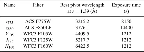
Table 1.HST imaging of XMMUJ2235-2557 used in this study. Name Filter Rest pivot wavelength Exposure time

atz=1.39 (Å) (s)

i775 ACS F775W 3215.2 8150

z850 ACS F850LP 3776.1 14400

Y105 WFC3 F105W 4409.5 1212

J125 WFC3 F125W 5217.7 1212

H160 WFC3 F160W 6422.5 1212

2 DATA

2.1 Sample

The cluster XMMUJ2235-2257 was serendipitously detected in an X-ray observation of a nearby galaxy by XMM-Newton and dis-covered by Mullis et al. (2005). Subsequent VLT/FORS2 spec-troscopy confirmed the redshift of the cluster to bez∼1.39. Rosati et al. (2009) confirmed the cluster membership of 34 galaxies. Among them 16 within the central 1 Mpc are passive. Jee et al. (2009) performed a weak-lensing analysis on the cluster and es-timated the projected mass of the cluster to be∼8.5×1014 M,

making it one of the most massive clusters seen at high-redshift. Grützbauch et al. (2012) studied the star formation in this cluster out to a projected radius of 1.5 Mpc and found that all massive galaxies have low specific star formation rates, and galaxies in the cluster centre have lower specific star formation rates than the rest of the cluster galaxies at fixed stellar mass. For the galaxy structural properties, this cluster has been investigated by Strazzullo et al. (2010) and was also included in the cluster sample of Delaye et al. (2014) and De Propris, Bremer & Phillipps (2015).

2.2 HSTimaging

We make use of the deep optical and IR archival imaging of the cluster XMMUJ2235-2557, obtained with HST/ACS WFC and

HST/WFC3 in June 2005 (PID 10698), July 2006 (PID 10496) and April 2010 (PID 12051). The ACS data are mostly from a program designed to search for Type Ia supernovae in galaxy clusters (Daw-son et al. 2009), while the WFC3 data are from a calibration pro-gram aiming at cross-calibrating the zero point of WFC3 and NIC-MOS. TheHST/ACS data consists of F775W and F850LP bands (hereafteri775andz850), while the WFC3 data comprises four IR

bands, F105W, F110W, F125W and F160W (hereafterY105,Y J110,

J125andH160). TheY J110data is not used in this study as it has a

shorter exposure time. The WFC3 data has a smaller field of view than the ACS data, 14500×12600. A summary of the observational setup can be found in Table 1.

Data in each band are reduced and combined using Astrodriz-zle, an upgraded version of the Multidrizzle package in thePyRAF

interface (Gonzaga et al. 2012). Relative WCS offsets between in-dividual frames are first corrected using thetweakregtask before drizzling. The ACS and WFC3 images have been drizzled to pixel scales of 0.05 and 0.09 arcsec pixel−1respectively. The full-width-half-maximum (FWHM) of the PSF is∼0.11 arcsec for the ACS data and∼0.18 arcsec for the WFC3 data, measured from median stacked stars. We produce weight maps using both inverse vari-ance map (IVM) and error map (ERR) settings for different purposes. TheIVMweight maps, which contain all background noise sources except Poisson noise of the objects, are used for object detection, while theERRweight maps are used for structural analysis as the

Poisson noise of the objects is included. Due to the nature of the drizzle process, the resulting drizzled images have correlated pixel-to-pixel noise. To correct for this we follow Casertano et al. (2000) to apply a scaling factor to the weight maps. Absolute WCS cal-ibrations of the drizzled images are derived using GAIA (Graph-ical Astronomy and Image analysis Tool) in the Starlink library (Berry et al. 2013) with Guide Star Catalog II (GSC-II) (Lasker et al. 2008).

3 ANALYSIS

3.1 Object detection, sample selection, and photometry

3.1.1 Method

The WFC3H160image, the reddest available band, is used for

ob-ject detection with SExtractor (Bertin & Arnouts 1996). The multi-band photometry is obtained with SExtractor in dual image mode with theH160image as the detection image.MAG_AUTOmagnitudes

are used for galaxy magnitudes and aperture magnitudes are used for colour measurements. We use a fixed circular aperture size of 100 in diameter. The effective radii of most galaxies in the clus-ter are generally much smaller than the aperture size. Galactic ex-tinction is corrected using the dust map of Schlegel, Finkbeiner & Davis (1998) and the recalibration E(B-V) value from Schlafly & Finkbeiner (2011).

As described in the introduction, Grützbauch et al. (2012) studied the star formation in the cluster out to a projected radius of 1.5 Mpc. We cross-match our SExtractor catalogue to theirs to identify spectroscopically confirmed cluster members from pre-vious literature (Mullis et al. 2005; Lidman et al. 2008; Rosati et al. 2009). 12 out of 14 spectroscopically confirmed cluster mem-bers are within the WFC3 FOV and identified. Figure 1 shows the colour-magnitude diagram of the detected sources within the WFC3 FOV. We identify passive galaxies through fitting the red se-quence from the colour-magnitude diagram. We measure the scat-ter through rectifying thez850−H160colour with our fitted relation,

then marginalise over theH160magnitude to obtain a number

distri-bution of the galaxies. The dotted lines correspond to±2σderived from a Gaussian fit to the number distribution.

Objects that are within 2σ from the fitted red-sequence are selected as the passive sample. We trim the sample by removing point sources indicated by SExtractor (i.e. those withclass_star >0.9) and applying a magnitude cut ofH160<22.5, which

cor-responds to a completeness of∼95% (see below). This selection results in a sample of 36 objects in the cluster XMMUJ2235-2557.

3.1.2 Quantifying the uncertainties on the photometry

Since the photometric uncertainties are folded directly into our mass estimates as well as the structural parameters measurements, a realistic estimate of the photometric uncertainties is required. Pre-vious works have shown that SExtractor tends to underestimate the photometric uncertainties and there can be a small systematic shift betweenMAG_AUTOoutput and the true magnitudes (Häussler et al. 2007). Hence, we perform an extensive galaxy magnitude and colour test with a set of 50000 simulated galaxies with sur-face brightness profiles described by a Sérsic profile on the ACS

z850and WFC3H160band images. This set of galaxies is also used

for assessing the completeness and accuracy of the light and mass structural parameter measurements. Details of the simulations can

20 21 22 23 0.0

0.5 1.0 1.5 2.0 2.5 3.0 3.5

20 21 22 23

H160 0.0

0.5 1.0 1.5 2.0 2.5 3.0 3.5

z850

−

H

160

Figure 1.Colour-magnitude diagram of the cluster XMMUJ2235. WFC3

H160magnitudes areMAG_AUTOmagnitudes while thez850−H160colour are 100aperture magnitudes. The dashed line corresponds to the fitted red sequence and the dotted lines are±2σ. Green circles correspond to objects that are included in our sample, which are within the dotted line and are not in the shaded area (i.e.H160<22.5). Objects that are spectroscopically confirmed cluster members from the catalogue of Grützbauch et al. (2012) are circled in dark red.

be found in Appendix A. Here we focus on the photometric uncer-tainties estimates.

The detection rate above a certain magnitude reflects the com-pleteness of the sample at that particular magnitude cut. We find that a magnitude cut ofH160<22.5 corresponds to a completeness

of∼95%. We then assess the accuracy of the recovered magnitudes and colours. Since the accuracies depend strongly on both input magnitude (magin) as well as the effective semi-major axis (ae) of

the galaxies, we assess the accuracy in terms of input mean surface brightness (Σ=magin+2.5 log(2πa2e)in mag arcsec−2) rather than

input magnitudes. Below we quote the results at a mean surface brightness of 23.5 mag arcsec−2inH160(or 24.5 mag arcsec−2in

z850) as a benchmark, as most objects we considered are brighter

than 23.5 mag arcsec−2_.

For ACSz850, the typical 1σ uncertainty for theMAG_AUTO

output at mean surface brightness of 24.5 mag arcsec−2 is∼0.33 mag. For WFC3H160, at a mean surface brightness of 23.5 mag

arcsec−2the typical 1σuncertainty is∼0.19 mag. Previous studies have shown that SExtractorMAG_AUTOmisses a certain amount of flux especially for the faint objects (e.g. Bertin & Arnouts 1996; Labbé et al. 2003; Taylor et al. 2009a). We find a systematic shift for both filters towards low surface brightness, the shifts are on average ∼0.42 mag for a H160 mean surface brightness of 23.5

mag arcsec−2or∼0.50 mag for az850mean surface brightness of

24.5 mag arcsec−2.

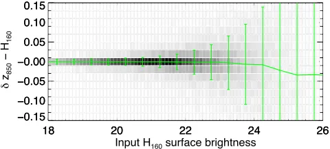
On the other hand, we find no systematics between the input and recovered aperture colour. Figure 2 shows the result for the

z850−H160colour from simulated galaxies. The uncertainties on

colour are small i.e.∼0.07 mag for aH160mean surface brightness

of 23.5 mag arcsec−2. The uncertainty in colour tends to be larger for objects with redderz850−H160colour, solely due to the fact that

thez850aperture magnitude has a larger uncertainty for a redder

colour.

18 20 22 24 26

−0.15 −0.10 −0.05 −0.00 0.05 0.10 0.15

18 20 22 24 26

Input H160 surface brightness −0.15

−0.10 −0.05 −0.00 0.05 0.10 0.15

δ

z850

−

H160

Figure 2.Differences between recovered and input aperture colourδz850−

H160= (z850−H160)out−(z850−H160)inas a function of input meanH160 surface brightness. The green line indicates the median and 1σdispersion in different bins (0.5 mag arcsec−2_{bin width), and the grey-shaded 2D} his-togram shows the number density distribution of the simulated galaxies.

3.2 Light-weighted structural parameters

3.2.1 Method

We measure the light-weighted structural parameters of the passive galaxies in five HST bands (i775,z850,Y105,J125andH160) using a

modified version of GALAPAGOS (Barden et al. 2012). For each object detected by SExtractor, GALAPAGOS generates a postage stamp and measures the local sky level around the object using an elliptical annulus flux growth method. This local sky level is then used by GALFIT (v.3.0.5, Peng et al. 2002), in order to model the galaxy surface brightness profile. We examine different settings of the sky estimation routine in GALAPAGOS to ensure the robust-ness of the results. Since the ACS and WFC3 images have a differ-ent spatial resolution, we modify GALAPAGOS to allow the use of a single detection catalogue (in our case, theH160band) in all

bands. The code is further adjusted to use the RMS maps derived from theERRweight maps output by Astrodrizzle.

As shown in Häussler et al. (2007), contamination by neigh-bouring objects has to be accounted while fitting galaxy surface brightness profiles, especially in regions where the object density is high. To deal with this issue, adjacent sources are identified from the SExtractor segmentation map and are masked out or fitted si-multaneously if their light profiles have a non-negligible influence to the central object. We fit a two-dimensional Sérsic profile (Sérsic 1963) to each galaxy, which can be written as

I(a) =Ieexp

−bn

(a ae

)1/n−1

(1)

where the effective intensityIecan be described by

Ie=

Ltot

2πnqa2

eb−n2nΓ(2n) (2)

whereΓ(2n)is the complete gamma function.

The Sérsic profile of a galaxy can be characterised by five in-dependent parameters: the total luminosityLtot, the Sérsic index n, the effective semi-major axisae, the axis ratioq(=b/a, where aand bis the major and minor axis respectively) and the posi-tion angleP.A.. The parameterbnis a function of the Sérsic index

(Γ(2n) =2γ(2n,bn), whereγis the incomplete gamma function)

and can only be solved numerically (Ciotti 1991). All five param-eters as well as the centroid (x,y) are left to be free parameters in our fitting process with GALFIT. The constraints of each parame-ter for GALFIT are set to be: 0.2<n<8, 0.3<ae<500 (pix),

0<mag<40, 0.0001<q<1,−180◦<P.A. <180◦. The sky

170

20 kpc

19 20 21 22 23 24 25 19 20 21 22 23 24 25 19 20 21 22 23 24 25

642

20 kpc

20 21 22 23 24 25 Σ / Mag arcsec−2

20 21 22 23 24 25 Σ / Mag arcsec−2

20 21 22 23 24 25 Σ / Mag arcsec−2

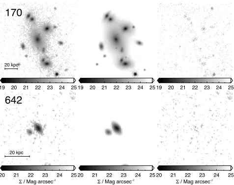
Figure 3.Examples of surface brightness profile fitting of two passive galaxies (ID 170, 642) in cluster XMMUJ2235-2557. From left to right:

H160galaxy image cut-out centered on the primary object, GALFIT best-fit models and residuals. The two examples are selected to demonstrate the clustering of sources. Galaxy 170, the BCG of this cluster is located in the central region of the cluster with high object density. Galaxy 642 is located in a more outer region of the cluster, yet is still affected by an extremely close neighbour. Multiple objects are fitted simultaneously as described in Section 3.2.1.

level on the other hand, is fixed to the value determined by GALA-PAGOS.

The Sérsic model is convolved with the PSF constructed from stacking bright unsaturated stars in the images. Note that we have also tried to derive aTinyTimPSF composite by adding PSF mod-els using theTinyTim code (Krist 1995) into the raw data and drizzling them as science images. Nevertheless, we notice that the

TinyTimdrizzled PSF does not match well the empirical PSF in the outer part: a much stronger outer envelope (as well as diffrac-tion spikes) can be seen in the empirical PSF (see also, Appendix A in Bruce et al. 2012, for a similar description). On the other hand, van der Wel et al. (2012) produced hybrid PSF models by replac-ing the central pixels of the median-stacked star by theTinyTim

PSF. We do not employ this correction as we find that the median-stacked star matches the TinyTim PSF reasonably well in the inner part.

The best-fitting light-weighted parameters are listed in Ta-ble F1 in Appendix F. Two galaxies (ID 170, 642) and their best-fits are shown in Figure 3 for illustrative purposes. These two objects have been chosen to show the impact of clustering of sources in dense regions. Even in the cluster centre where there are multiple neighbouring objects, GALFIT can do a good job in determining the structural parameters by fitting multiple object simultaneously. Below we discuss the reliability and uncertainties in these light-weighted structural parameters.

3.2.2 Reliability of the fitted structural parameters

GALAPAGOS coupled with GALFIT performs well in most cases. However in some exceptions, it is rather tricky to obtain a good-quality fit due to various issues. We are not referring here to the global systematics and uncertainties (which are addressed in the next section), but on stability and quality control of individual fits. We find that using an inadequate number of fitting components for

the neighbouring sources (due to inadequate deblending in the SEx-tractor catalogue or appearance of extra structures / sources in bluer bands, e.g.z850band, compare to ourH160detection catalogue) can

lead to significant residuals that adversely affect the fit of the pri-mary object. Similarly, since GALAPAGOS fits sources with a sin-gle Sérsic profile by default, GALFIT will likely give unphysical outputs for unresolved sources / stars in the field (withaehitting

the lower boundary of the constraintae=0.3 pix, or Sérsic index

hitting the upper boundaryn=8) or even not converging in these cases, which again affects the result of the object of primary in-terest. Moreover, the best-fit output can vary if we use a different treatment for neighbouring sources. We notice that in a few cases the results can be very different depending upon whether neigh-bouring sources are masked or are fitted simultaneously.

To ensure high reliability, we perform the following checks for each galaxy: 1) We visually inspect the fits as well as the seg-mentation maps (output by SExtractor) in each band to ensure ad-jacent sources are well-fitted. Extra Sérsic components are added to poorly fitted neighbouring objects iteratively if necessary. 2) For neighbours for which GALFIT gives ill-constrained results (i.e. hit-ting the boundaries of the constraints), we replace the Sérsic model with a PSF model and rerun the fit, which often improves the con-vergence and the quality of the best-fit model. Regarding this, Bar-den et al. (2012) explained the need of fitting Sérsic profiles to sat-urated stars instead of PSF model in GALAPAGOS, since the PSF often lacks the dynamic range to capture the diffraction spikes of the bright saturated stars. In our case this is not necessary since there are only a few bright saturated stars in the field, for which we can safely mask their diffraction spikes. 3) We compare the re-sults of masking and simultaneously fitting neighbouring objects. In most cases the two methods give results that are within 1σ. For galaxies with close neighbours (e.g. within 5ae) we prefer to fit

them simultaneously as any inadequate or over-masking can result in problematic fits, judging by examining the residual map output by GALFIT. On the other hand, masking is more suitable when the neighbouring object are not axisymmetric or show certain substruc-tures, which causes the single Sérsic fit to not reach convergence.

3.2.3 Quantifying the uncertainties in light-weighted structural parameters

We quantify the systematic uncertainties using the set of 50000 simulated galaxies inserted on the images. In this section we fo-cus on the result of the test; details of the simulations can be found in Appendix A3. Note that the uncertainties quoted here are more likely to represent lower limits to the true uncertainties, as the sim-ulated galaxies are also parametrised with a Se´rsic profile.

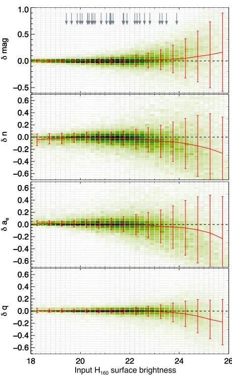
Figure 4 shows the comparison between the input and recov-ered magnitudes and structural parameters for theH160band. The

magnitudes recovered by Sérsic profile fitting are accurate with almost no systematics and a 1σ dispersion less than 0.25 for ob-jects having meanH160surface brightness brighter than 23.5 mag

arcsec−2_{. The Sérsic index, effective radius and axis ratio}

measure-ments are generally robust for objects brighter than a meanH160

surface brightness of 23.5 mag arcsec−2. The bias between the re-covered and input Sérsic indices is less than 8% and the 1σ disper-sion is lower than 30%. Effective radii have a bias less than 4% and a 1σdispersion lower than 30% for objects brighter thanH160

sur-face brightness of 23.5 mag arcsec−2. For objects with high mean surface brightness (i.e.<19 mag arcsec−2) in our simulated sam-ple, the effective radii are slightly overestimated (∼2%) and the Sérsic indices are underestimated (∼ −4%) by GALFIT. We find

18 20 22 24 26 −0.5

0.0 0.5 1.0

18 20 22 24 26

I t H f b i ht

−0.5 0.0 0.5 1.0 δ mag −0.5 0.0 0.5 1.0 δ mag

18 20 22 24 26

−0.6 −0.4 −0.2 0.0 0.2 0.4 0.6

18 20 22 24 26

I t H f b i ht

−0.6 −0.4 −0.2 0.0 0.2 0.4 0.6 δ n −0.6 −0.4 −0.2 0.0 0.2 0.4 0.6 δ n

18 20 22 24 26

−0.6 −0.4 −0.2 0.0 0.2 0.4 0.6

18 20 22 24 26

I t H f b i ht −0.6 −0.4 −0.2 0.0 0.2 0.4 0.6 δ ae −0.6 −0.4 −0.2 0.0 0.2 0.4 0.6 δ ae

18 20 22 24 26

−0.6 −0.4 −0.2 0.0 0.2 0.4 0.6

18 20 22 24 26

I t H f b i ht

−0.6 −0.4 −0.2 0.0 0.2 0.4 0.6 δ q −0.6 −0.4 −0.2 0.0 0.2 0.4 0.6 δ q

18 20 22 24 26

−0.6 −0.4 −0.2 0.0 0.2 0.4 0.6

18 20 22 24 26

Input H160 surface brightness

−0.6 −0.4 −0.2 0.0 0.2 0.4 0.6 δ q −0.6 −0.4 −0.2 0.0 0.2 0.4 0.6 δ q

Figure 4.Differences between recovered and input structural parameters by GALFIT in function of input meanH160surface brightness. From top to bottom: magnitudeδmag=magout−magin, Sérsic indicesδn= (nout−

nin)/nin, effective semi-major axesδae= (ae−out−ae−in)/ae−inand axis ratioδq= (qout−qin)/qin. Red line indicates the median and 1σ disper-sion in different bins (0.5 mag arcsec−2bin width) and green-shaded 2D histogram shows the number density distribution of the simulated galaxies. The grey arrows indicate theH160surface brightness of the galaxies in our cluster sample.

out that this bias is due to unresolved objects in our simulations. A related discussion can be found in Appendix A3.

We have also performed the same test on a simulated back-ground similar to the actual images (where the main difference is that the simulated background has no issue of neighbour contam-ination), and find that the uncertainties on the effective radius are on average∼15−20% lower compared to those derived from real images.

For each galaxy in the sample, we compute the meanH160

sur-face brightness and add the corresponding dispersion in quadrature to the error output by GALFIT.

3.3 Elliptical aperture photometry and color gradients

In addition to structural parameters, we derivez850−H160colour

profiles for the passive sample with PSF-matched elliptical annular

photometry. We first convert the 2D image in both bands into 1D radial surface brightness profiles. Morishita et al. (2015) demon-strated that deriving 1D profiles with elliptical apertures has certain advantages over circular apertures. Profiles derived with concentric circular apertures are biased to be more centrally concentrated. We perform an elliptical annular photometry on the PSF-matchedz850

andH160images at the galaxy centroid derived from GALFIT. The

GALFIT best-fit axis ratios and position angles of individual galax-ies (inH160band) are used to derive a set of elliptical apertures for

each galaxy.

Due to the proximity of objects in the cluster, it is necessary to take into account (as in 2D fitting) the effect of the neighbour-ing objects. The neighbourneighbour-ing objects are first removed from the image by subtracting their best Sérsic fit (or PSF fit in some cases) in both bands. While the fit might not be perfect, we find that this extra step can remove the majority of the flux of the neighbouring objects contributing to surface brightness profiles. For some galax-ies the colour profiles show substantial change after we apply the correction.

We then measure the colour gradients of individual galaxies by fitting the logarithmic slope of theirz850−H160colour profiles

along the major axis, which are defined as follows:

z850−H160=∇z850−H160×log(a) +Z.P. (3)

At redshift 1.39 this corresponds roughly to the rest-frame(U−R)

colour gradient. The depth and angular resolution of our WFC3 data allow us to derive a 1D colour profile accurately to∼3−4ae,

hence the colour gradient is fitted in the radial range of PSF half-width-half-maximum (HWHM)<a<3.5 ae. We note that the

colour gradients of most galaxies, as well as the median colour gra-dient, do not strongly depend on the adopted fitting radial range. Figure 5 shows the colour profiles and logarithmic gradient fits of four passive galaxies as an example. The colour profiles are in gen-eral well-described by logarithmic fits.

3.4 Stellar mass-to-light ratio – colour relation

We estimate the stellar mass-to-light ratios of the cluster galaxies in XMMUJ2235-2557 using an empirical relation between the ob-servedz850−H160colour and stellar mass-to-light ratio (M∗/L). At

redshift 1.39, thez850−H160colour (rest-frameU−R) straddles

the 4000 break. Hence, this colour is sensitive to variations in the properties of the stellar population (i.e. stellar age, dust and metal-licity). In addition, the effects of these variations are relatively de-generate on the colour -M∗/Lplane (almost parallel to the relation,

Bell & de Jong 2001; Bell et al. 2003; Szomoru et al. 2013), which makes this colour a useful proxy for theM∗/L.

We derive the relation using the NEWFIRM medium band sur-vey (NMBS) catalogue, which combines existing ground-based and space-based UV to mid-IR data, and new near-IR medium band NEWFIRM data in the AEGIS and COSMOS fields (Whitaker et al. 2011). The entire catalogue comprises photometries in 37 (20) bands, high accuracy photometric redshifts derived withEAZY

(Brammer, van Dokkum & Coppi 2008) and spectroscopic redshifts for a subset of the sample in COSMOS (AEGIS). Stellar masses and dust reddening estimates are also included in the catalogue, and are estimated by SED fitting usingFAST(Kriek et al. 2009).

To derive theM∗/L-colour relation, we use the stellar masses

from the NMBS catalogue in COSMOS estimated with stellar pop-ulation models of Bruzual & Charlot (2003), an exponentially de-clining SFHs, and computed with a Chabrier (2003) IMF. We do not use the sample in AEGIS as it contains photometries with fewer

0.5 1.0 1.5 2.0 2.5

z850

−

H

160

552

552

∇z − H = −0.777±0.092

0.5 1.0 1.5 2.0 2.5

z850

−

H

160

296

296

∇z − H = −0.392±0.110

0.5 1.0 1.5 2.0 2.5

z850

−

H

160

588

588

∇z − H = −0.605±0.035

−1.5 −1.0 −0.5 0.0 0.5 log(a/a_e)

0.5 1.0 1.5 2.0 2.5

z850

−

H

160

170

170

∇z − H = −0.133±0.038

Figure 5.Examples of colour profile fitting of four passive galaxies in the cluster XMMUJ2235-2557. From top to bottom: colour profiles for galaxies ID 552, 296, 588 and 170 (with log(M∗/M) =10.46, 10.54, 10.81, 11.81) along the logarithmic major axis (log(a/ae). The grey line in each panel is the elliptical-averagedz850−H160colour profile. Regions that are fitted (PSF HWHM<a<3.5ae) are over-plotted in black. The vertical black dotted and dashed line show the minimum (PSF HWHM) and maximum radial distance for fitting (3.5ae). The error bars show the error on the mean of thez850−H160colour at each distance. The blue solid line is the best logarithmic gradient fits, and the blue dotted-dashed lines are the±1σ

error of the slope.

bands. We derive the relation in the observer frame and compute the observedz850−H160colour for all NMBS galaxies. Note that we

do not adopt the typical approach to interpolate the cluster data to obtain a rest-frame colour (e.g. with InterRest, Taylor et al. 2009b) due to limited availability of bands, which would likely lead to de-generacy in choices of templates. Firstly, we rerun EAZYfor all NMBS galaxies to obtain the best-fit SED template, these SEDs are then integrated with the ACSz850 and WFC3H160filter

re-sponse for thez850−H160colour. Similarly we obtain the

luminos--1.4 -1.2 -1.0 -0.8 -0.6 -0.4 -0.2 0.0

1.29 < z < 1.49

-1.4 -1.2 -1.0 -0.8 -0.6 -0.4 -0.2 0.0

log (M

*

/LH

160

)

718 Objects

0.0 0.5 1.0 1.5 2.0 2.5

z850−H160 −0.4

−0.2 0.0 0.2 0.4

δ

log (M

*

/LH

160

)

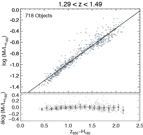
Figure 6.Relation between stellar mass-to-light ratio and z-H colour at red-shift∼1.39 using the public NMBS catalogue. Gray points are 718 galaxies from the NMBS catalogue that satisfy the selection criteria. Black line is the best-fit linear relation. Bottom panel shows the residuals of the relation

δlog(M∗/LH160) =data - linear fit in colour bins of 0.1.

ityLH160of each galaxy in the observedH160band, from which we

calculate the stellar mass-to-light ratioM∗/LH160. We select NMBS

galaxies within a redshift window of 0.1 of the cluster redshift, i.e. 1.29<z<1.49, and apply the magnitude cut (H160<22.5) and a

chi-square cut (χ2<2.0, from template fitting inEAZY) to better match the cluster sample.

A total of 718 objects are selected by this criterion. A redshift correction is applied to these 718 galaxies to redshift their spec-tra to the cluster redshift (i.e. similar to k-correction in observer frame). We then measure theirz850−H160colour andLH160 in the

observer frame. This redshift correction is effective in reducing the scatter of the relation, indicating that some of (but not all) the scat-ter is simply due to difference in redshifts. Figure 6 shows the fitted relation between log(M∗/LH160) andz850−H160colour. The black

line is the best-fit linear relation with:

log((M∗/LH160)/(M/L)) =0.625(z850−H160)−1.598 (4)

The relation is well-defined within a colour range of 0.4<

z850−H160<2.2 (hence we choose the same range for our

sim-ulated galaxies, see Appendix A). The global scatter of the fit is

∼0.06 dex. In the lower panel of Figure 6 we plot the residuals of the fit in colour bins of 0.1. The uncertainty in log(M∗/L) is

generally<0.1 in each bin and the bias is negligible. The remain-ing scatter results from redshift uncertainties and stellar population variations (age, dust and metallicity), as their effects are not exactly parallel to the relation. Note that this can lead to small systematics in measuring mass-to-light ratios and the mass-to-light ratio gradi-ents. For example in metal-rich or old regions the mass-to-light ra-tio will likely be systematically slightly underestimated, and over-estimated in metal-poor or young regions (Szomoru et al. 2013).

3.5 Integrated stellar masses

We estimate the integrated stellar masses (M∗) of the cluster

galax-ies using ourM∗/L-colour relation, thez850−H160aperture colours

and the total luminosityLH160from best-fit Sérsic models. The

un-certainties in stellar mass comprise photometric unun-certainties in the colour andH160 luminosity, as well as the scatter in the derived

colour -M∗/L relation. The typical uncertainty of the masses is ∼0.1 dex, comparable to the uncertainties obtained from SED fit-ting.

Previous literature computed SED mass with multi-band

MAG_AUTOphotometry obtained with SExtractor (e.g. for this clus-ter, Strazzullo et al. 2010; Delaye et al. 2014). Nevertheless, as we have shown in Section 3.1.2, it is known that MAG_AUTOcan be systematically biased, due to the assumption in SExtractor that the sky background comprises only random noise without source con-fusion (Brown et al. 2007). Hence, more recent studies use the to-tal luminosity from best-fit Sérsic models to correct the masses to account for the missing flux inMAG_AUTO (Bernardi et al. 2013; Bezanson et al. 2013). In our case, we have demonstrated that total luminosity from the best-fit Sérsic models can recover input galaxy magnitudes to a high accuracy. Hence, we scale our masses with the total luminosityLH160 from best-fit Sérsic models rather than

H160MAG_AUTOmagnitudes. We also compute masses withH160

MAG_AUTO; the difference between the two is small for our sample, withhM∗,MAG_AU T O−M∗,Sersici=−0.039 dex.

For this particular cluster, Delaye et al. (2014) estimated the galaxies masses through SED fitting with four bands (HST/ACS

i775,z850, HAWK-IJ,Ks), which also gave an uncertainty of∼0.1

dex in mass. The masses derived with our method are consistent with the SED masses in Delaye et al. (2014) within the uncertain-ties. A comparison of masses estimated usingM∗/L-colour

rela-tion with masses computed using SED fitting can be found in Ap-pendix C. The uncertainty of the absolute stellar masses is of course larger (as in the case of SED fitting), depending on the details of NMBS SED fitting and e.g. choice of IMF.

3.6 Resolved stellar mass surface density maps

We further exploit theM∗/L-colour relation to derive stellar mass

surface density maps. This allows us to study the mass distribution within each galaxy, at the same time eliminating the effect of inter-nal colour gradient which influences the light-weighted size mea-surements. Below we describe the main steps involved in deriving stellar mass surface density maps with theM∗/L-colour relation.

3.6.1 PSF matching

We first match the resolution of the ACSz850image (∼0.100) to the

WFC3H160image (∼0.1800). PSF matching is critical in this kind

of study as the measured colour has to come from the same phys-ical projected region. We stack the unsaturated stars for each band to obtain characteristic PSFs, then generate a kernel that matches thez850toH160PSF using thepsfmatchtask in IRAF. The

differ-ence between the resultantz850PSF and theH160PSF is less than

2.5%. Details of the PSF matching can be found in Appendix B. We then apply the kernel to the ACSz850image. The PSF matched

z850image is resampled to the same grid as theH160image using

the software SWarp (Bertin et al. 2002). We then generate postage stamps of each galaxy in bothH160and PSF matchedz850images

for deriving resolved stellar mass surface density maps.

3.6.2 From colour to stellar mass surface density

The next step is to convert the z850−H160 colour information

into mass-to-light ratios with theM∗/L-colour relation described

in Section 3.4. Nevertheless, a direct pixel-to-pixel conversion is not possible for our data. The conversion requires a certain min-imum signal-to-noise (S/N) level because: a) significant biases or massive uncertainties may arise if colours are not well mea-sured. b) our relation is only calibrated within the colour range of 0.4<z850−H160<2.2. Any low S/N colour that falls outside the

calibrated range could convert to an unphysicalM∗/L.

Therefore, we adopt the Voronoi binning algorithm as de-scribed by Cappellari & Copin (2003), grouping pixels to a tar-get S/N level of 10 per bin. For each galaxy, we run the Voronoi binning algorithm on the sky-subtracted PSF-matchedz850 band

postage stamps as a reference, as it has a lower S/N compared to the

H160image. The same binning scheme is then applied to the

sky-subtractedH160 image. The subtracted sky levels are determined

by GALAPAGOS. The two images are then converted into magni-tudes. Binnedz850−H160colour maps are obtained by subtracting

the two. We then construct a binnedM∗/Lmap by converting the

colour in each bin to a masstolight ratio with the derived colour

-M∗/Lrelation.

An extrapolation scheme is implemented to determine the

M∗/Lin regions or bins with insufficient S/N, for example in the

galaxy outskirts and the sky regions. We first run an annular av-erage to derive a 1-dimensional S/N profile inz850for individual

galaxies using the light-weighted galaxy centroid, axis ratio and position angle determined in Section 3.2. For the area outside the elliptical radius that has a S/N less than half of our target S/N (i.e. S/N∼5), we fix theM∗/Lto the annular median ofM∗/Lbins at

the last radius with sufficient S/N. We find that this extrapolation is crucial for the following structural analysis as the sky noise is preserved (see the discussion in Appendix A4).

We construct resolved stellar mass surface density maps (here-after referred to as mass maps) by directly combining the extrap-olatedM∗/L map and the original (i.e. unbinned)H160 images.

Figure 7 illustrates the procedure of deriving mass maps from the

z850andH160images. Using the originalH160image instead of the

binned one allows us to preserve the WFC3 spatial resolution in the mass maps. Note that in theory combining a binned (i.e. spa-tially discrete)M∗/Lmap with a smooth luminosity image would

result in a discrete mass profile in low S/N region, in order words, induce an “discretization effect" in the mass maps. This effect is more severe in low S/N regions, i.e. the galaxy outskirts where the bins are larger (hence less smooth). For bright galaxies, since there are more bins with sufficient S/N and the dynamical range of the light distribution (surface brightness gradient) is much larger than theM∗/Lgradient, this appears to have minimal effect and does

not largely affect our result. For fainter galaxies this issue is non-negligible. To tackle this, for each galaxy we perform the above binning procedure 10 times, each with a slightly different set of initial Voronoi nodes. This ends up with a set ofM∗/Lmaps which

are then median-stacked to create the final mass map. This extra step alleviates the discretization effect.

3.7 Mass-weighted structural parameters

3.7.1 Method

We measure mass-weighted structural parameters from the re-solved stellar mass surface density maps. We follow a similar procedure as with the light-weighted structural parameters, using

GALFIT to model the mass profiles with two-dimensional Sérsic profiles. All five parameters of the Sérsic profile (M∗,tot,n,ae,q

andP.A.) and the centroid (x,y) are left to be free parameters in the fit. We use the same GALFIT constraints as for the light-weighted structural parameters, except for allowing a larger range for the Sér-sic indices: 0.2<n<15.0. This is because the mass profiles are expected to be more centrally peaked compared to light profiles (Szomoru et al. 2013). As theH160 images are background

sub-tracted before being converted into mass maps, the sky level (i.e. the mass level) is fixed to zero in the fitting process. The best-fitting mass-weighted parameters are given in Appendix F1.

3.7.2 Quantifying the uncertainties in mass-weighted parameters

We further assess the accuracy of our mass conversion procedures as well as the reliability of the mass-weighted structural parameter measurements. The details of the test are described in Appendix A4. Similar to the uncertainty in the light-weighted parameters, the uncertainties quoted here are more likely to represent lower limits to the true uncertainties.

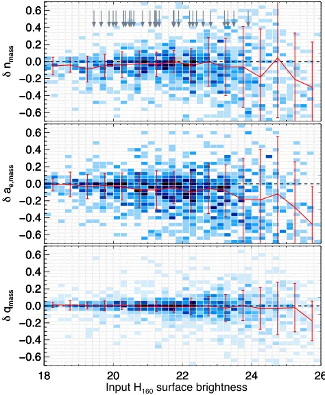
Figure 8 shows the difference between input and recovered mass-structural parameters as a function ofH160surface brightness.

The Sérsic index, effective radius and axis ratio measurements are generally robust for objects brighter thanH160surface brightness

of 23.5 mag arcsec−2. This is important, as it demonstrates that our mass conversion procedure does not significantly bias the re-sult. The bias between the recovered and input Sérsic indices is less than 7% and the 1σ dispersion is lower than 40%, and

effec-tive radii have a bias less than 10% and a 1σdispersion lower than 40%. Among the three parameters, the axis ratio can be recovered most accurately. Compared with the light uncertainties (Figure 4), the mass uncertainties in all parameters are∼2 times higher. Sim-ilar to the light-weighted parameters, for each galaxies we add the corresponding dispersion in quadrature to the error output by GAL-FIT.

We find that for a couple of objects the fits do not converge, or have resultant sizes smaller than the PSF size. To avoid biases and wrong conclusions we remove these objects that are not well-fitted from the mass parameter sample. 6 objects (out of 36) are discarded, among them one object is spectroscopically confirmed. Three of them initially have small light-weighted sizes and their fitted mass-weighted sizes become smaller than half of the PSF HWHM, which are unreliable (see the discussion in Appendix A3). Most of them are low mass galaxies (i.e. log(M∗/M)<10.5).

3.7.3 Deviation of mass-weighted parameters - 1D vs. 2D

Szomoru et al. (2013) derived 1D mass profiles from 1D radial sur-face brightness profiles and measured mass-weighted structural pa-rameters. In theory, fitting in 1D and in 2D should give identical results, as statistically fitting an averaged smaller group of points and fitting all the points without averaging are equivalent (see, Peng 2015, for a detailed discussion.). Nevertheless, in practice deriving maps and fitting in 2D have certain advantages: a) It does not rely heavily on the Sérsic profile fitting in light. Deriving elliptical aver-aged profiles require a predetermined axis ratio and position angles, which, in our case, come from the light Sérsic profile fitting. This will of course fold in the uncertainties of these two parameters into the 1D profiles, which complicates the propagation of uncertainties in the mass-weighted parameters. b) In the cluster region, the ob-ject density is high and many galaxies have very close neighbours.

Hence it will be more appropriate to fit all the sources simulta-neously to take into account the contribution from the neighbour-ing objects, rather than derivneighbour-ing 1D profile without deblendneighbour-ing the neighbouring contamination. A possible way to solve this is to first subtract the best-fit 2D models of the neighbours from the 2D im-ages before generating the 1D profiles, but of course this depends strongly on how well the neighbours can be subtracted, and still suffer from a).

4 LOCAL COMPARISON SAMPLE

In order to study the evolution of mass-weighted sizes over red-shift, we compare our cluster sample atz∼1.39 to a local sam-ple of passive galaxies from the Spheroids Panchromatic Investiga-tion in Different Environmental Regions (SPIDER) survey (La Bar-bera et al. 2010b). The publicly available SPIDER sample includes 39993 passive galaxies selected from SDSS Data Release 6 (DR6), among them 5080 are in the near-infrared UKIRT Infrared Deep Sky Survey-Large Area Survey Data release (UKIDSS-LAS DR4) in the redshift range of 0.05 to 0.095. La Barbera et al. (2010b) de-rived structural parameters in all available bands (grizY JHK) with single Sérsic fitting with2DPhot(La Barbera et al. 2008).

We use the structural parameters ing-band andr-band from the publicly available multiband structural catalogue from La Bar-bera et al. (2010b) to derive mass-weighted structural parameters. For the galaxy selection, we follow similar criteria as La Barbera et al. (2010b): we apply a magnitude cut at the 95% completeness magnitude (Mr6−20.55), aχ2cut from the Sérsic fit for bothg -band andr-band (χ2<2.0), and a seeing cut at61.5”. This results in a sample of 4050 objects. We compute integrated masses for the sample as in Section 3.5 with apertureg−rcolour. The colours are obtained from direct numeral integration of theg-band andr-band Sérsic profiles to 5 kpc instead of using GALFIT total magnitudes. Extending the integration limit to larger radius (e.g. 10 kpc) does not change largely the derived masses. With theg−rcolour we de-rive and select red-sequence galaxies within 2σfollowing the same method discussed in Section 3.1; we end up with a sample of 3634 objects (hereafter the SPIDER sample). On top of that we use the group catalogue from La Barbera et al. (2010c) to select a subsam-ple of galaxies residing in high density environments. Applying a halo mass cut to the SPIDER sample of log(M200/M)>14, we

end up with a subsample of 627 objects (hereafter the SPIDER clus-ter sample), which we will use as the main comparison sample for our high-redshift cluster galaxies.

2D Sérsic model images ing-band andr-band are then gen-erated with fitted parameters from the structural catalogue. Given the large number and relatively low object density of local galaxies compared to our high redshift cluster sample, using fitted parame-ters from the structural catalogue is statistically reliable and issues mentioned in Section 3.7.3 do not contribute substantially here. We construct mass maps for individual galaxies using the procedure described in Section 3.6.2 without Voronoi binning and stacking. A

M∗/L-colour relation is again derived from the NMBS sample as in

Section 3.4, but ing-band andr-band at 0<z<0.27, a window of 0.2 in redshift around the median redshift of the SPIDER sample. A total of 1315 NMBS objects are selected. The mass maps are then fitted with GALFIT to obtain mass-weighted structural parameters.

296

10 kpc

19 20 21 22 23 24 25

z850

20 21 22 23 24 25 26

H160

19 20 21 22 23 24 25 0.6 0.8 1.0 1.2 1.4 1.6 0.04 0.13 0.21 0.306.5 7.0 7.5 8.0 8.5 9.0 9.5 6.5 7.0 7.5 8.0 8.5 9.0 9.5 6.5 7.0 7.5 8.0 8.5 9.0 9.5

308

10 kpc

19 20 21 22 23 24 25

Σ / Mag arcsec−2

z850

20 21 22 23 24 25 26

Σ / Mag arcsec−2

H160

19 20 21 22 23 24 25

Σ / Mag arcsec−2

0.6 0.8 1.0 1.2 1.4 1.6 z850 − H160

0.10 0.15 0.20 0.25

M*/L / MO • /LO •

6.5 7.0 7.5 8.0 8.5 9.0 9.5 log(Σ / MO • kpc

-2 )

6.5 7.0 7.5 8.0 8.5 9.0 9.5 log(Σ / MO • kpc

-2 )

6.5 7.0 7.5 8.0 8.5 9.0 9.5 log(Σ / MO • kpc

-2 )

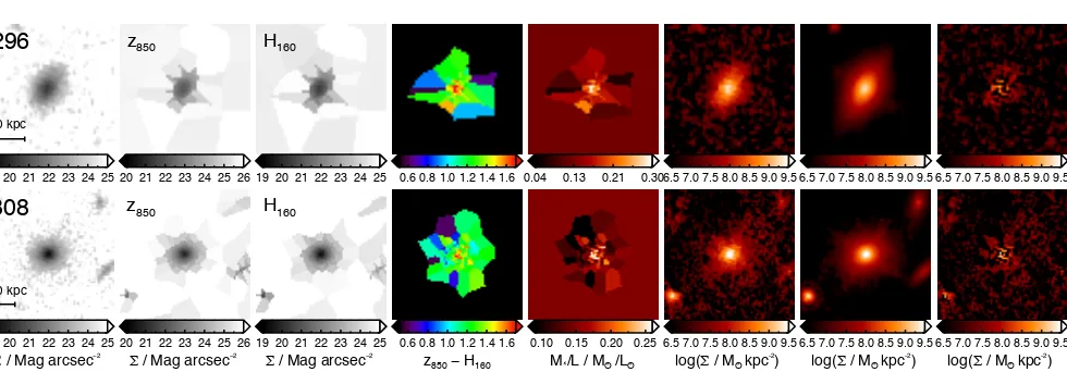
Figure 7.Examples of mass map derivation and fitting of two passive galaxies (ID 296, 308) in cluster XMMUJ2235-2557. From left to right:H160galaxy image cut-outs centred on the primary object, Voronoi-binnedz850images, Voronoi-binnedH160images,z850−H160colour maps,M∗/L, the surface mass density mapsΣmass, the GALFIT best-fit models and residuals in mass. Bins that are extrapolated are masked out (shown in black) in the colour maps. The procedure is described in detail in Section 3.6.2.

5 RESULTS

5.1 Wavelength dependence of light-weighted galaxy sizes

The measured size of a galaxy depends on the observed wave-length, as different stellar populations are being traced at differ-ent wavelength (e.g., the “morphological k-correction”, Papovich et al. 2003). With our multi-band measurements of light-weighted structural parameters of the cluster passive galaxies, we first inves-tigate the wavelength dependence of galaxy sizes at this redshift. This wavelength dependence of sizes (or the size-wavelength rela-tion) has been quantified for local passive galaxies in a number of studies (e.g. Barden et al. 2005; Hyde & Bernardi 2009; La Bar-bera et al. 2010b; Kelvin et al. 2012; Vulcani et al. 2014; Kennedy et al. 2015). The dependence shown by the above mentioned stud-ies is quite strong, in the sense that galaxy sizes can decrease up to∼38% fromgthroughKband in the GAMA sample (Kelvin et al. 2012), or∼32% across the same range in SPIDER (La Bar-bera et al. 2010b). Nevertheless, different authors disagree on the extent of the reduction in sizes in various datasets. For example, in a recent study Lange et al. (2015) revisited the GAMA sample with deeper NIR imaging data and found a smaller size decrease,∼13% fromgtoKsband.

At higher redshift, study of wavelength dependence of sizes is scarce in clusters. The star formation history and age gradient may contribute significantly to the size-wavelength dependence, for ex-ample the inside-out growth scenario suggests that younger stellar population are more widespread compared to the older population in the core of passive galaxies. Various authors have shown that measured sizes in the observed optical and NIR (i.e. rest-frame UV vs rest-frame optical for high-redshift galaxies) show a difference of∼20–25% (e.g. Trujillo et al. 2007; Cassata et al. 2010; Dam-janov et al. 2011; Delaye et al. 2014), although some find no differ-ence (Morishita, Ichikawa & Kajisawa 2014). The comparisons are usually done with only two bands, hence it is unclear whether this dependence can change with redshift. Recent works from CAN-DELS studied the wavelength dependence of sizes for 122 early-type galaxies (ETG) in the COSMOS field in three HST bands (F125W, F140W and F160W) at redshift 0<z<2, and found an average gradient ofdlog(ae)/dlog(λ) =−0.25 independent of mass and redshift (van der Wel et al. 2014).

Figure 9 shows the change in size with rest-frame wavelength for our sample. Here we use the light-weighted effective semi-major axisaefrom GALFIT, as the galaxy size. We assume every

galaxy in the sample is at the cluster redshift. We select 28 galaxies (out of 36) with no problematic fits in any of the five bands. The fraction of problematic fits is larger ini775andY105due to shorter

exposure time and lower throughput of the filter, which result in lower S/N. To facilitate comparison with the literature, the sizes in figure 9 are normalised with the medianH160sizes of our sample,

which is approximately equal to the rest-framer-band size. We plot the best-fitting relation for local spheroids by Kelvin et al. (2012) and the SPIDER cluster sample, normalised in the same way, for comparison. We see a smooth variation of sizes decreasing from

i775toH160bands (rest-frameutor). The reduction in the median

size (fromi775toH160) is∼20%, which is consistent with the

ex-pected decrease across this wavelength range (∼19%) following the relation of Kelvin et al. (2012) and the SPIDER cluster sample (La Barbera et al. 2010b). The average size gradient of our sample from the best-fit power law isdlog(ae)/dlog(λ) =−0.31±0.27.

We also attempt to divide the sample in mass bins as in Lange et al. (2015) to investigate the size change with wavelength for different masses. Lange et al. (2015) showed that the size re-duction decreases from ∼13% for local passive galaxies with log(M∗/M) =10.0 to∼11% for those with log(M∗/M) =11.0.

On the other hand, van der Wel et al. (2014) reported no dis-cernible trends with mass in CANDELS. We split the sample in half at the median mass (log(M∗/M)610.6 and log(M∗/M)>

10.6, 14 objects per bin), plotted in grey and slate grey in Fig-ure 9. A steeper dependence can be seen for the high mass bins (dlog(ae)/dlog(λ) =−0.57±0.28) compared to the whole sam-ple, while the low mass bins (dlog(ae)/dlog(λ) =−0.29±0.34)

have the same if not slightly shallower wavelength dependence within the uncertainties. This is the opposite to the finding of Lange et al. (2015). Nevertheless, the size gradients of the two bins are within 1σ, a larger sample is needed to confirm the mass depen-dence.

18 20 22 24 26 −0.6 −0.4 −0.2 0.0 0.2 0.4 0.6

18 20 22 24 26

Input H160 surface brightness

−0.6 −0.4 −0.2 0.0 0.2 0.4 0.6 δ q −0.6 −0.4 −0.2 0.0 0.2 0.4 0.6 δ q

18 20 22 24 26

−0.6 −0.4 −0.2 0.0 0.2 0.4 0.6

18 20 22 24 26

Input H_F160W surface brightness

−0.6 −0.4 −0.2 0.0 0.2 0.4 0.6 δ qmass −0.6 −0.4 −0.2 0.0 0.2 0.4 0.6 δ qmass

18 20 22 24 26

−0.6 −0.4 −0.2 0.0 0.2 0.4 0.6

18 20 22 24 26

Input H160 surface brightness

−0.6 −0.4 −0.2 0.0 0.2 0.4 0.6 δ ae,mass −0.6 −0.4 −0.2 0.0 0.2 0.4 0.6 δ ae,mass

18 20 22 24 26

−0.6 −0.4 −0.2 0.0 0.2 0.4 0.6

18 20 22 24 26

Input H_F160W surface brightness

−0.6 −0.4 −0.2 0.0 0.2 0.4 0.6 δ nmass −0.6 −0.4 −0.2 0.0 0.2 0.4 0.6 δ nmass

Figure 8.Differences between recovered and input mass-weighted struc-tural parameters by GALFIT as a function of inputH160surface brightness. Similar to Figure 4, but for mass-weighted structural parameters. From top to bottom: Sérsic indicesδn= (nout−nin)/nin, effective semi-major axes

δae= (ae−out−ae−in)/ae−inand axis ratioδq= (qout−qin)/qin. Red line indicates the median and 1σdispersion in different bins (0.5 mag arcsec−2 bin width) and blue-shaded 2D histogram shows the number density distri-bution of the simulated galaxies. The grey arrows indicate theH160surface brightness of the galaxies in our cluster sample.

5.2 Stellar mass – light-weighted size relation

In this section we show the stellar mass –H160light-weighted size

relation of the cluster XMMUJ2235-2557. The mass-size relation of this cluster (inz850band, rest-frame UV) has been studied in

previous literature (Strazzullo et al. 2010; Delaye et al. 2014). In the top panel of Figure 10 we plot the mass – size re-lation for the passive popure-lation in the cluster selected from red sequence fitting. Circled objects are spectroscopically confirmed cluster members (Grützbauch et al. 2012). The size we use from this point onwards is the circularised effective radius (Re−circ),

de-fined as:

Re−circ=ae×

√

q (5)

whereaeis the elliptical semi-major radius andq=b/ais the axis

ratio from the best-fit GALFIT Sérsic profile.

The integrated stellar masses are derived from theM∗/L

-colour relation and are scaled with the total GALFIT Sérsic magni-tude (see Section 3.5 for details). We also plot the local mass-size relation for the SDSS passive sample by Bernardi et al. (2012) for comparison. We note that although this relation was derived for galaxies regardless of their local density, a number of studies have established that there is no obvious environmental dependence on passive galaxy sizes in the local universe (Guo et al. 2009; Wein-mann et al. 2009; Taylor et al. 2010; Huertas-Company et al. 2013;

3000

4000

5000

6000 7000

−

0.1

0.0

0.1

0.2

3000

4000

5000

6000 7000

Rest wavelength (

λ

/ Å)

−

0.1

0.0

0.1

0.2

log(a

/ a

)

SPIDER (log(M200/MO •)≥ 14) Kelvin et al. 2012 log(M*/MO •) ≤ 10.6 log(M*/MO •) > 10.6

Figure 9.Size-wavelength relation of the passive galaxies in the cluster XMMUJ2235-2557. Black circles show the median sizes of the sample in each band positioned at the rest-frame pivot wavelength, normalised with the medianH160-band sizes (approximately rest-framer-band, ae,r). Er-ror bars show the uncertainty of the median in each band, estimated as 1.253σ/

√

N, whereσ is the standard deviation andN is the size of the sample. The best-fit power law to the sizes in our sample is shown as a red dashed line. The green dot-dashed line is the best-fit relation for the SPI-DER cluster sample (fromg-band toKs-band), while the green diamonds are the median size of the sample ing-band andr-band, normalised in the same way. The blue dotted line is the best-fit relation for local galaxies from Kelvin et al. (2012). Grey and slate grey are the median sizes for two mass bins (log(M∗/M)610.6 and log(M∗/M)>10.6) respectively.

Cappellari 2013). We pick the single Sérsic fit relation in Bernardi et al. (2012) for consistency, which is shown to have slightly larger sizes than the two-component exponential + Sérsic fit relation.

Hyde & Bernardi (2009) first demonstrated that the mass-size relation of passive galaxies shows curvature and Bernardi et al. (2012) fitted the curvature with a second order polynomial; their best-fit values were consistent with Simard et al. (2011). As we have shown in the last section, size shows wavelength-dependence, hence care has to be taken to ensure the sizes being compared are at around the same rest-frame wavelength. The Bernardi et al. (2012) local relation is based on the Sloanr-band, while our sizes are mea-sured in theH160band at a redshift of 1.39, which roughly

corre-sponds to the same rest-frame band. As a result, no size-correction is required as the correction tor-band is negligible.

TheH160 band sizes of the passive galaxies in this cluster

are on average∼40% smaller than expected from the local re-lation by Bernardi et al. (2012) with hlog(Re−circ/RBernardi)i=

−0.21 (∼45% smaller for the spectroscopic confirmed members,

hlog(Re−circ/RBernardi)i=−0.25). There are also galaxies whose

sizes are ∼70% smaller than those of their local counterparts (log(Re−circ/RBernardi) =−0.56). As one can see from Figure 10,

the most massive object in the cluster is the BCG, which also has the largest size (∼24 kpc) and lies on the local relation. This is consistent with findings from Stott et al. (2010, 2011), who showed that as a population, BCGs have had very little evolution in mass or size sincez∼1. Tiret et al. (2011) suggested that major mergers at

z>1.5 are required to explain the mass growth of these extremely

massive passive galaxies. Hence below we exclude the BCG when fitting the mass-size relation. We fit the mass-size relation with a Bayesian inference approach using Markov Chain Monte Carlo (MCMC; Kelly 2007) with the following linear regression:

log(Re−circ/k pc) =α+β(log(M∗/M)−10.5) +N(0,ε) (6) whereN(0,ε)is the normal distribution with mean 0 and dispersion ε. Theεrepresents the intrinsic random scatter of the regression.

The best-fit parameters (the interceptα, slopeβ and the

scat-terε) for both the entire red-sequence selected sample (A) and the spectroscopically confirmed members only (B) are summarised in Table 2. For mass completeness and comparison to previous litera-ture, we also fit only the massive objects with log(M∗/M)>10.5,

the limiting mass adopted in Delaye et al. (2014) (C & D). We no-tice that the slope of the relation can change by more than 1σ de-pending on the considered mass range. We also fit the slope using the elliptical semi-major axisaeinstead ofRe−circ), which gives us

a significantly flatter slope (β=0.35±0.15).

Our measured slope is consistent at the 1σ level with the results of Delaye et al. (2014), who studied the mass-size rela-tion using seven clusters at 0.89<z<1.2 in the rest-frame B -band (i.e. β =0.49±0.08 for log(M∗/M)>10.5). Papovich

et al. (2012) measured the sizes of passive galaxies in a cluster at

z=1.62 and found that ETG with masses log(M∗/M)>10.48

have hRe−circi=2.0 kpc with the interquartile percentile range

(IQR) of 1.2−3.3 kpc. Sizes in XMMUJ2235-2557 are on aver-age 40% larger (hRe−circi=2.80 kpc, IQR=1.45−4.38 kpc).

While the fits are consistent with each other on a 1σ level, we notice that the relation in Delaye et al. (2014) for this cluster is flatter (β=0.2±0.3) compared to both our full sample fit (A) and massive sample fit (C). This difference could be due to a combina-tion of a) their mass-size relacombina-tion is computed in thez-band while ours is inH160, b) the two red sequence samples are selected

differ-ently and c) the masses computed here are scaled with total GAL-FIT Sérsic magnitude instead ofMAG_AUTO(the relation is slightly flatter:β=0.38±0.27 instead of 0.43 if we use the masses scaled

withMAG_AUTO).

A caveat of the above comparison is that we have not consid-ered the effect of progenitor bias (van Dokkum & Franx 2001). Cor-recting the progenitor bias (in age and morphology) has been shown to reduce the magnitude of the observed size evolution (Saglia et al. 2010; Valentinuzzi et al. 2010a; Beifiori et al. 2014). Recently, Jørgensen et al. (2014) corrected the progenitor bias by removing galaxies that are too young in the Coma cluster to be the descen-dants of a cluster atz=1.27 and found no size evolution with red-shift.

5.3 Colour gradients in the passive cluster galaxies

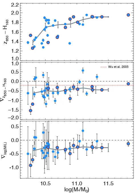
In Figure 11 we show the 100 aperture colour, colour gradients

∇z850−H160 and log(M∗/L)gradients∇log(M/L)of the passive

sam-ple as a function of stellar mass. The log(M∗/L)gradients are

de-rived from fitting 1DM∗/Lprofiles, which are derived from 1D

colour profiles using theM∗/L-colour relation. Note that since the

M∗/L-colour relation is essentially a one-to-one mapping,

measur-ing the colour gradient is qualitatively equivalent to measurmeasur-ing the log(M∗/L)gradient.

More massive galaxies appear to have a redder z850−

H160 colour, as also shown by Strazzullo et al. (2010) with

HST/NICMOS data. Redder colour implies a higher medianM∗/L

from theM∗/L-colour relation. The passive sample has a range of

−0.5 0.0 0.5 1.0 1.5

log(R

e

−

circ

/kpc)

Full passive sample fit

Bernardi et al. 2012 H160

0.5 PSF HWHM

10.5 11.0 11.5

−0.5 0.0 0.5 1.0 1.5

log(R

e

−

circ

/kpc)

Full passive sample fit (Light−weighted)

Full passive sample fit (Mass−weighted)

log(M*/MO •)

0.5 PSF HWHM

Mass

Figure 10. Stellar mass – size relations of the passive galaxies in XMMUJ2235-2557. Top: with light-weighted sizes. Green dots show the sample selected with the passive criteria described in Section 3.1. Spectro-scopically confirmed objects are circled with dark red. The green line is a linear fit to the full passive sample (Case A), while the dot-dashed lines rep-resent±1σ. The dark grey line corresponds to the localr-band mass-size relation from Bernardi et al. (2012). Bottom: with mass-weighted sizes. In-dividual objects are shown in orange. The orange solid line corresponds to the full sample fit (Case A) for the mass– mass-weighted size relation, and the orange dot-dashed lines represent±1σ. The green line is the same linear fit in the top panel for comparison. The BCG is indicated with the black diamond. The cross shows the typical uncertainty of the sizes and the median uncertainty of the integrated mass in our sample.

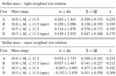
Table 2.Best-fit parameters of the Stellar mass – size relations Stellar mass – light-weighted size relation

Case Mass range α±∆α β±∆β ε

A 10.06M∗611.5 0.263±1.441 0.359±0.135 0.235 B 10.06M∗611.5 (spec) 0.329±2.096 0.138±0.192 0.195 C 10.56M∗611.5 0.114±1.876 0.576±0.173 0.195 D 10.56M∗611.5 (spec) 0.149±2.935 0.447±0.268 0.175 Stellar mass – mass-weighted size relation

Case Mass range α±∆α β±∆β ε

A 10.06M∗611.5 0.074±1.733 0.240±0.162 0.235 B 10.06M∗611.5 (spec) 0.037±2.467 0.141±0.227 0.212 C 10.56M∗611.5 −0.043±2.093 0.477±0.192 0.182 D 10.56M∗611.5 (spec) −0.152±3.839 0.411±0.350 0.209