ABSTRACT
HITE, JASON MICHAEL. Bayesian Parameter Estimation for the Localization of a Radioactive Source in a Heterogeneous Urban Environment. (Under the direction of John Mattingly).
This dissertation presents a new approach to localizing an unknown source of radiation in an urban environment using a distributed detector network. The method employs Bayesian statistical parameter estimation techniques, relying on an approximation for the response of a detector to the source using a simplified model of the underlying transport phenomena based on ray-tracing, combined with a Metropolis-type sampler that is modified to propagate the effect of fixed epistemic uncertainties in the material cross sections of objects in the scene. This method is first demonstrated with simulated measurements generated primarily using a geometry derived from a real city block, with the algorithm able to localize an 8.7 mCi source to within a few
meters based on observations from 6 detectors with a 10 scount time. These results also show
that the effect of uncertainties in the material cross sections on the precision of the localization is relatively weak, implying that precise estimates of the composition of objects in the scene are not necessary.
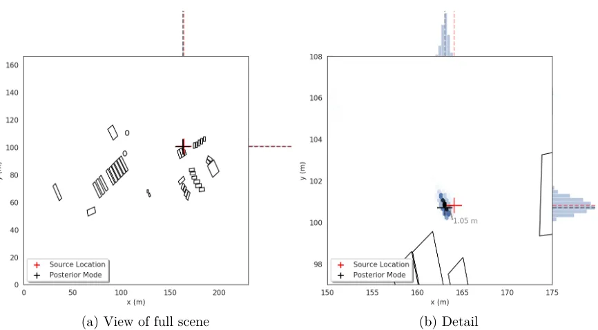
Results from these simulated tests were used to design a field measurement campaign con-ducted in cooperation with Oak Ridge National Laboratory in a scene mimicking a typical ur-ban setting. After extending the simplified detector model to account for the orientation of the detectors, analysis of these measurements shows that the algorithm is able to localize a37 mCi
source to within ∼2 mfor30 min measurements in two separate trials, though the results also
suggest that count times as short as 5 minare sufficient.
© Copyright 2019 by Jason Michael Hite
Bayesian Parameter Estimation for the Localization of a Radioactive Source in a Heterogeneous Urban Environment
by
Jason Michael Hite
A dissertation submitted to the Graduate Faculty of North Carolina State University
in partial fulfillment of the requirements for the Degree of
Doctor of Philosophy
Nuclear Engineering
Raleigh, North Carolina 2019
APPROVED BY:
Ralph Smith Yousry Azmy
Daniel Archer John Mattingly
DEDICATION
BIOGRAPHY
ACKNOWLEDGEMENTS
This would not have been possible without the input of everyone I have worked with throughout the years. Thanks especially to my committee and my fellow students, as well as my adviser John Mattingly, who stood up for me.
TABLE OF CONTENTS
List of Tables . . . vii
List of Figures . . . .viii
Chapter 1 Introduction . . . 1
1.1 Motivation and Applications . . . 4
1.2 Prior and Related Work . . . 7
1.3 Novel Contributions . . . 9
Chapter 2 Bayesian Statistics and MCMC . . . 10
2.1 Bayes’ Rule . . . 10
2.2 Markov Chains . . . 11
2.3 Markov Chain Monte Carlo . . . 20
2.3.1 The Metropolis-Hastings Algorithm . . . 21
2.4 Special Considerations . . . 25
2.4.1 Convergence Rate and Burn-in . . . 25
Chapter 3 Methodology for Source Localization . . . 29
3.1 Markov-Chain Monte Carlo Sampling . . . 30
3.2 Statistical Model for Detector Response . . . 32
3.3 Detector Response Model . . . 33
3.3.1 Effect of Detector Orientation . . . 36
3.4 Propagation of Cross Section Uncertainties . . . 36
3.5 Adaptive Metropolis . . . 37
3.6 Complete Algorithm for Source Localization . . . 38
3.6.1 Relation to Maximum Likelihood Estimation . . . 40
3.6.2 Difficulties with Direct Numerical Optimization . . . 40
Chapter 4 Preliminary Experiments in Simulated Geometry . . . 42
4.1 Synthetic Model in Urban Geometry . . . 43
4.2 Comparison to High-Fidelity Simulation . . . 45
4.3 Effect of Cross Section Uncertainties on Localization Error . . . 47
4.4 Informing the Design of a Field Experiment . . . 50
Chapter 5 Field Test . . . 52
5.1 Description of Experiment . . . 52
5.1.1 Detector Placement . . . 54
5.1.2 Detector Characteristics . . . 56
5.1.3 Site Characterization . . . 58
5.2 Results and Analysis . . . 60
5.2.1 Detector orientation . . . 64
5.2.2 Count rate anomalies during measurements . . . 66
5.2.4 Other Sources of Error . . . 69
5.2.5 Trilateration . . . 70
Chapter 6 Effects of detector anomalies, signal-to-noise ratio, and alternative physics models . . . 72
6.1 Anomaly Classifier . . . 73
6.2 Dependence on Source Intensity . . . 80
6.3 Occluded Detector Model . . . 83
Chapter 7 Conclusions. . . 90
7.1 Summary of Major Results . . . 91
LIST OF TABLES
Table 3.1 Model parameters. . . 34 Table 4.1 Predicted source locations and standard deviations for marginal posterior . 49 Table 5.1 Summary of actual source and detector placement during the experiment,
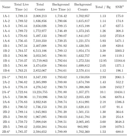
including a qualitative description of the visibility of the source for each detector. . . 56 Table 5.2 Count rates recorded by the detectors. Entries marked with a (∗) denote
measurements with anomalous count rates (see Section 5.2.2). Total-to-background ratios and SNRs are adjusted for live time. . . 61 Table 5.3 Predicted source locations using simple trilateration with error estimates
without accounting for detector orientation. . . 71 Table 5.4 Predicted source locations using simple trilateration with error estimates
including detector orientation. All distances are in meters. . . 71 Table 6.1 Classifier results for Experiment 1. . . 76 Table 6.2 Classifier results for Experiment 2. Highlighted rows correspond to the
LIST OF FIGURES
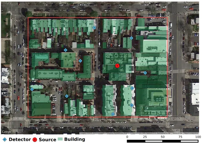
Figure 1.1 Example source localization problem, with a detector network distributed over a city block. We wish to determine the location of the source using
only count rates measured by the detectors. . . 2
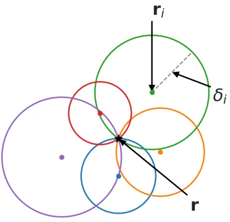
Figure 1.2 Illustration of trilateration; source is located at the point where circles overlap. . . 3
Figure 1.3 Illustration of trilateration with uncertainty; source lies somewhere inside the black circle. . . 4
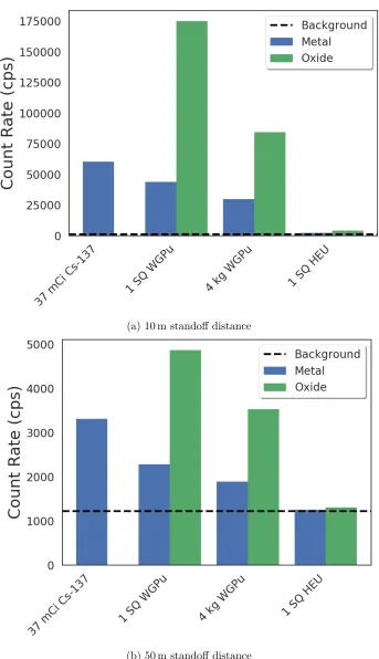
Figure 1.4 Count rates for various sources of interest, simulated usingGADRAS-DRF for a 2”×4”×16”NaI detector. . . 6
Figure 2.1 States x1 and x2 are reachable from x0, x0 is not reachable from x1 or x2,x1 and x2 form a closed communicating class. . . 15
Figure 2.2 Graphs depicting reducible and irreducible Markov chains. . . 16
Figure 2.3 Example of a periodic chain, the example trajectory shows that statesx0 and x3 are visited with a period of 3. . . 17
Figure 2.4 Limiting behavior of probability mass in a periodic chain. . . 18
Figure 2.5 Trace plots showing typical behavior of chains as they approach convergence 27 Figure 2.6 Behavior of Gelman-Rubin scores for chains in Fig. 2.5 . . . 28
Figure 3.1 Visual illustration of the ray tracing procedure . . . 35
Figure 3.2 Sum-of-squares error as a function of source location for experiment 1 described in Chapter 5. The peaks are clipped to show detail of the error surface. . . 41
Figure 4.1 Satellite image of test location, with modeled geometry overlayed in green, as well as source (red) and detector (blue) locations. . . 44
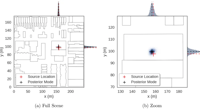
Figure 4.2 Posterior density for source location in synthetic experiments. . . 45
Figure 4.3 Model geometry used for simulations using MCNP. . . 46
Figure 4.4 Posterior density for localization based on simulations with MCNP. . . 47
Figure 4.5 Posterior density for source location with 5% uncertainty in all cross sec-tions. . . 48
Figure 5.4 Model geometry of the site, colored by the calculated mean free path. The DGPS reference points are also indicated by the black marks. Note that there are some small disagreements with the objects visible in the satellite imagery, this is due to the satellite photos being taken on a different day
than that of the experiments. . . 59
Figure 5.5 Elevation difference in experiment 2. The source is located just behind the fence visible in the background. . . 60
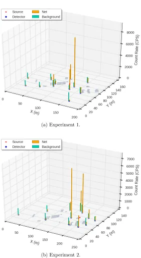
Figure 5.6 Foreground and background count rates in both experiments. . . 62
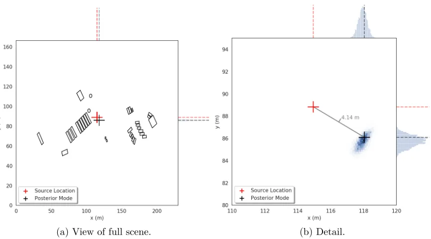
Figure 5.7 Marginal posterior density for source locationrin experiment 1 with 50% relative uncertainty in all cross-sections. . . 63
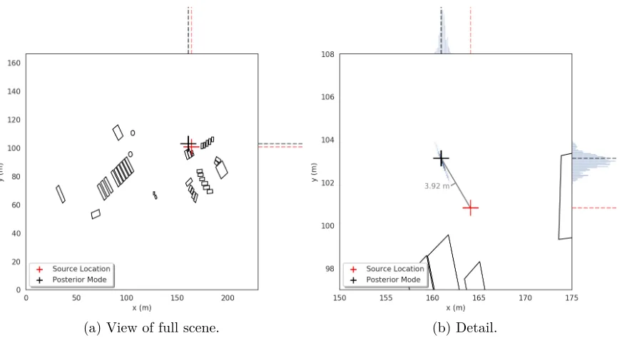
Figure 5.8 Marginal posterior density for source locationrin experiment 2 with 50% relative uncertainty in all cross-sections. . . 64
Figure 5.9 Marginal posterior density for source locationrin experiment 1 with 50% relative uncertainty in all cross-sections and including detector orientation. 65 Figure 5.10 Marginal posterior density for source locationrin experiment 2 with 50% relative uncertainty in all cross-sections and including detector orientation. 65 Figure 5.11 Time series of fluctuating count rates recorded by three of the detectors in experiment 2 (blue) versus the average count rate over the entire mea-surement (green). . . 67
Figure 5.12 Marginal posterior density for source locationrin experiment 2 with 50% relative uncertainty in all cross-sections, including detector orientation and with counts from anomalous detectors removed. . . 68
Figure 5.13 Error in estimated source location versus count time for experiment 1. . . 69
Figure 6.1 Illustration of count rate models for different types of anomalies. . . 74
Figure 6.2 1A-1,Kp = 0.002. Constant. . . 77
Figure 6.3 1B-5,Kp= 1.557. Constant, but borderline. Some linear trend is visible, but is not significant enough to reject a constant trend. . . 77
Figure 6.4 2A-1,Kp = 2.321. Linear. . . 78
Figure 6.5 2A-3, Kp = 0.090. Constant. Despite the clear drop in count rate near the start, classification indicates overall trend is constant. . . 78
Figure 6.6 2A-4,Kp = 29.345. Step. . . 79
Figure 6.7 2B-6,Kp= 5.437. Step. . . 79
Figure 6.8 Plot of localization error with various source activities. . . 81
Figure 6.9 Posterior density with varying source intensity. . . 83
Figure 6.10 Occluded model, 4 detectors with line-of-sight to the source. . . 86
Figure 6.11 Attenuating model, 4 detectors with line-of-sight to the source. . . 86
Figure 6.12 Occluded model, 2 detectors with line-of-sight to the source. . . 87
Figure 6.13 Attenuating model, 2 detectors with line-of-sight to the source. . . 87
Figure 6.14 Occluded model, 1 detector with line-of-sight to the source. . . 88
Figure 6.15 Attenuating model, 1 detector with line-of-sight to the source. . . 88
Figure 6.16 Occluded model, no detectors with line-of-sight to the source. . . 89
Chapter 1
Introduction
This dissertation describes a new method for locating an unknown source of radiation in a heterogeneous environment. A source is assumed to exist in the search area1 (referred to as the
Figure 1.1: Example source localization problem, with a detector network distributed over a city block. We wish to determine the location of the source using only count rates measured by the detectors.
As a simple example, I will demonstrate what is perhaps the simplest method for localizing a source, generally known astrilateration. Assume for simplicity that the source and detectors are constrained to a plane and that the environment is a vacuum with no background. In this case, the mean count rate recorded by the i-th detector, di due to an isotropic and monoenergetic
source of known activityI, located at positionr, is given by2
di(r, I) =i· I 4πkr−rik22
, (1.1)
whereriis the detector location andiis the total efficiency of the detector, withi= 1,2, ..., ND.
Let us denote the distance between the source and detector as δi = kr−rik2, where k ◦ k2
is the Euclidean norm of a vector. Given a particular dˆi measured by the detector, we can
solve Eq. (1.1) for δi = 2 q
πdˆi/Ii. Given several detectors, we can draw a set of circles,
each centered on ri with radius δi; the source is then localized by finding the intersection
of these circles (Fig. 1.2). More precisely, we can solve the linear least-squares problem given
2We can extend the method shown here to estimate the activity of the source, but the system of equations
by Eq. (1.2), which will have a unique solution whenND ≥33 [25].
2 (ri−rND)
|r=kr
ik22− krNDk
2
2−δ2i +δN2D i= 1,2, . . . , ND−1 (1.2)
Figure 1.2: Illustration of trilateration; source is located at the point where circles overlap.
Figure 1.3: Illustration of trilateration with uncertainty; source lies somewhere inside the black circle.
This simple example also ignores the possibility of objects in the scene, which will attenuate the radiation emitted by the source at different rates, as well as the presence of background radiation, which adds random noise to the measurements. Accounting for the presence of at-tenuators greatly complicates estimation of the detector responses, generally resulting in a non-linear (as well as non-smooth and non-convex) system of equations which must be solved using advanced iterative techniques [41]. Prior work in this area has tended to focus on source local-ization in the absence of attenuators (or ignoring their effect), while the method presented in this dissertation incorporates a simplified model for the transport of radiation in a heteroge-neous medium.
1.1 Motivation and Applications
the more recent 2013 theft of a cobalt-60 source used for medical teletherapy near Hueypoxtla, Mexico [27] highlight the need for methods that can aid in the identification and location of radioactive sources over a large area.
My analysis is focused primarily on searching for sources which are significant sources of gamma radiation. This is due to the scale of interest; at the scale of a city block most other forms of radiation will quickly be attenuated to levels that are not measurable with readily-available detectors. The experiments described in subsequent chapters have generally employed millicurie amounts of cesium-137 with a characteristic gamma ray energy of 662 keV, arising from β
-decay to an excited state of barium-137 and the subsequent relaxation to the ground state. While cesium-137 is itself a source of concern, with the NTI reporting at least 4 proliferation-significant incidents involving cesium-137 in 2012, I also consider it as a stand-in for other sources of interest, including special nuclear material (SNM). Figure 1.4 plots simulations of the count rates recorded in a2”×4”×16”NaI detector at standoff distances of10 mand50 m,
with simulations performed usingGADRAS-DRF[31]. Count rates are shown for the37 mCisource
(a)10 mstandoff distance
(b)50 mstandoff distance
1.2 Prior and Related Work
Localizing an emissive source based on the measured signal strength of a network of detectors is a topic that has been widely investigated, with a large variety of algorithms described in the literature. As was briefly mentioned earlier, the simplest method is via trilateration, where the signal strength reported by each detector is used to infer a distance from the source to the detector. This creates a set of overlapping circles, each centered on a detector, with radius given by the predicted distance from the source to the corresponding detector. The source is then localized by finding the point of intersection for the set of circles.
This method is perhaps best illustrated in ref. [36], which uses trilateration with a1/distance2
model for the detector count rates to estimate the source location, and a variance-weighted average to estimate source activity. The authors demonstrate that the algorithm is able to accurately localize a 0.95µCi cesium source, though the distance scale of the experiments is
small (∼1 m) and the scene is free of obstructions. Trilateration is also well-known outside
of the nuclear engineering community, with ref. [25] presenting an overview of applications to the localization of nodes in a wireless network; it also forms the basis of the Global Positioning System [23, Ch. 2].
Many other authors present work that can be interpreted in a similar framework to that of ref. [36], where localization is fundamentally achieved using a 1/distance2 model for the
count rates recorded by each detector as a function of source location and intensity, see for example refs. [5, 32, 33, 34]. One shortcoming is that these formulations do not attempt to account for the presence of attenuating material in the scene, with the 1/distance2 model
equivalent to assuming the scene is a homogeneous or a vacuum. More cluttered scenes may however contain objects such as buildings or vehicles, which significantly affect the count rates measured by detectors– an effect that is not accounted for by 1/distance2 models. To my
contribution of scattered gammas to the detector response is substantial.
Another distinguishing characteristic of existing localization algorithms is in the statistical parameter estimation techniques used. The classic solution to the statistical parameter estima-tion problem is themaximum likelihood estimate(MLE), which is defined as the collection of source parameters that maximizes the statistical likelihood of observing the measured de-tector responses. MLE methods are very popular in many applications due to their robustness and the reliability of modern numerical optimization algorithms. They have seen wide applica-tion, with ref. [33] demonstrating the use of an MLE for a detector response model dependent on the source activity and the distance from the source to the detector. Recent work has also applied MLE to the complementary problem of estimating the spatial and temporal distribu-tion of background and subsequently using this estimate to detect an anomalous source using a mobile detector network [26].
Bayesian techniques have also seen a growth in usage in recent years, enabled largely by the increasing computational resources available to researchers. Ref. [19] provides an early example, deriving amaximum a posterioriestimator (conceptually similar to an MLE, but formulated in a Bayesian context) of the source location intended for use in real-time tracking. Using a Gaussian noise state model, the authors show that their estimator is able to track a cesium-137 source in real-time as it moves throughout a 10 m×15 m room. The results presented therein
show the algorithm has good performance, being able to track the source to within a few inches as it is moved around, but does not include a detailed description of the experiments. Most notably, the source activity is not stated, though from the distance scale involved it would be reasonable to assume a source in the 100µCi to500µCi range was used.
There also exists a separate class of Bayesian algorithms collectively known asparticle fil-ters. This approach can be understood as a type of genetic algorithm, where several “particles” are distributed throughout the search space, with each particle representing a candidate source location. Measured data is used to determine the fitness of each particle by computing its like-lihood and the system is evolved to produce a new generation of particles; over several gener-ations, the particles tend to cluster around the true source location. This method has proven especially useful in online monitoring, with ref. [35] demonstrating the algorithm applied to a vehicle portal monitoring scenario.
method is able to detect and characterize 4 sources simultaneously without prior knowledge of the number of sources, though the presence of attenuating objects in the scene is not considered. Ref. [42] also provides valuable insight into some of the practical aspects of operating a detector network for source localization. This work proposes methods for dealing with the spatial errors present in measurements recorded by a detector network, as well as for variations in the efficiency of individual detectors. Such errors arise from issues of time synchronization between detectors as well as errors in the position information derived from GPS measurements, and are expected to occur in any real-world measurements. These practical considerations are important to field deployment of any wide-area localization algorithm, particularly when using low-cost mobile radiation detectors where high-accuracy GPS location information is not available, as well as in sensor networks that rely on multiple different types of detector.
1.3 Novel Contributions
Chapter 2
Bayesian Statistics and MCMC
In this chapter, I will outline the mathematical theory underlying the method for source local-ization that is the focus of this dissertation. I will begin with a description of Bayesian statis-tics while noting some of the difficulties involved with their direct application, followed by a description of the key properties of Markov chains. I will then show how these properties can be used to construct a procedure known as Markov chain Monte Carlo (MCMC), which enables the practical usage of Bayesian techniques, and conclude with some discussion of their convergence. In subsequent chapters I will specialize this methodology to the problem of source localization, as well as reexamine the material discussed here in more qualitative terms.
Note that the material presented in this chapter is not novel, and is included for the sake of completeness of presentation. In particular, I have drawn heavily on ref. [40] and ref. [24] in compiling the material shown here, while providing my own perspective on the portions relevant to the problem of source localization.
2.1 Bayes’ Rule
Imagine that we are presented with a random variable X, with corresponding sample space S. X is characterized by an unknown probability density function (PDF) p(x). Here, p(x) is
a probability measure defined on event space F, where F is the σ-algebra of S (the set of all
subsets of S measurable underp). We will assume that we are provided with realizations ofX,
say{xi}Ni=0−1, which can be observed without knowingp(x). Intuitively you might suspect that
if we continue to observe realizations of X we may be able to reconstruct p in a form that is
representative of the behavior we have observed.
we “update” our state of knowledge to incorporate the new information. First, consider that we begin with an initial state of knowledge encoded as a PDF, which I will refer to as the prior
orprior densityand denote asp0(x). We seek theposterior density,p(x|x0), which is the
conditional probability of x given that we have observed x0, incorporating the observation x0
into our knowledge aboutX.
To determine how we might compute p(x|x0), first recall one of the fundamental axioms of
probability. Consider two arbitrary eventsA, B ∈ S, then [3, Eq. 16.39]:
Pr[A∧B] =Pr[A]·Pr[B|A]
=Pr[B]·Pr[A|B]. (2.1)
That is to say, the probability thatAand Boccur is the product of the probability ofAand the
conditional probability of B given A, i.e. the probability B occurs given that A has occurred
(and vice-versa). We can equate the right-hand sides of Eq. (2.1) and solve for Pr[A|B]:
Pr[A]·Pr[B|A] =Pr[B]·Pr[A|B]
Pr[A|B] = Pr[A]·Pr[B|A]
Pr[B] .
(2.2)
Equation (2.2) is often known as Bayes’ rule and provides exactly what we are after– the conditional probability of observingA given that we have previously observedB. Expressed in
terms of probability densities and substituting our prior and posterior forX:
p(x|x0) =
p(x0|x)·p0(x)
R
Sp(x0|x)·p0(x)dx
. (2.3)
2.2 Markov Chains
Definition 2.2.1 (Stochastic process).LetX ={Xt; t∈ T }denote a sequence of random
variables on a common probability space (S,F, p), where S is the sample space of X, F is
theσ-algebra ofS (known as theevent space ofX),pis a probability measure overF, andT
is a totally ordered index set. The sequence X is known as a stochastic processorrandom process. If the index set T is taken as a subset of the integers thenX is known as adiscrete time stochastic process, whereas if it is taken as a sub-interval of the real numbers thenX is
referred to as a continuous time stochastic process. Similarly, if the state space S is finite
or countably infinite then X is known as a discrete state stochastic process, otherwise it is
typically referred to as acontinuous state stochastic process.
We call each index in the set T a step in the process; this notation was selected because
it is most common that these steps correspond to a procedure where we sequentially observe the evolution of a random system in time. In this context we typically refer to the actual value observed at stept∈ T,xt∈ S (a realization of Xt) as the stateof X at step t, while S is the state space ofX.
In the interest of simplicity, we will limit our discussion here to finite state and countable
time stochastic processes, where S is a finite set and T is countable. Similar results hold in
in continuous time and countably infinite state spaces but the analysis is significantly more involved, so we will rely on the theory of discrete processes to illustrate the concepts [39]. We are also primarily interested in one particular type of stochastic process, the Markov chain. Loosely speaking, Markov chains are stochastic processes that lack “memory”– their state at timet dependsonly on the state at timet−1. More formally:
Definition 2.2.2 (Markov Chain). LetX ={Xt; t∈ T }be a stochastic process on a given
probability space (S,F, p). We consider here only the case that X is a discrete time and finite
state stochastic process. X is called a Markov chain if it possesses the Markov property,
namely that, for all t∈ T:
Pr[Xt=xt|X0 =x0, X1 =x1, . . . , Xt−1 =xt−1] =Pr[Xt=xt|Xt−1=xt−1]. (2.4)
A Markov chain is a random sequence characterized by a state spaceS, which is the common
gij :=Pr[Xt+1 =xj|Xt=xi]. These gij’s may in general depend on tbut I will assume it does
not, which is referred to as a time-homogeneous Markov chain. Intuitively, this implies that at any point we can “reset” the chain and begin again from any particular state, since
gij : =Pr[Xt+1=xj|Xt=xi] =Pr[X1 =xj|X0 =xi].
(2.5)
Since we have assumed finite S we can form the matrix of gij’s, G = [gij], which is called
thetransition kernelof the chain. If we letp(0) be a row vector1 representing the probability mass function ofX0, then we can calculatep(1) =p(0)Gto determine the probability mass
func-tion of X1. If we further define thek-step transition probabilitygijk :=Pr[Xt+k =xi|Xt=xj],
with correspondingGk, then we can calculate the probability mass function for any stepXtas
follows:
p(t)=p(t−1)G
=p(t−2)GG
· · ·
=p(0)Gt.
(2.6)
We are most interested in the properties of the chain relating to the evolution of the proba-bility mass astis advanced. These are dictated primarily by the transition probabilities, hence
we will study the relationship between Gand p(t) in some detail. Our main item of interest is the stationary distribution of the chain, which (if it exists) is a distribution that is a fixed point ofG.
Definition 2.2.3 (Stationary Distribution).For a Markov chain with state space S and
where convergence is understood to be in the weak sense (convergence in distribution). The existence of this limit is not guaranteed, though when it does exist the following relations must hold [40, Sec. 4.6]:
πππ= lim t→∞p
(t)
= lim t→∞p
(0)G(t)
= lim t→∞p
(0)G(t+1)
=
lim t→∞p
(0)G(t)G
=πππG.
(2.8)
Thus if the limit exists then πππ is also a stationary distribution of the chain. As mentioned,
this limit is not guaranteed to exist and even when it does the resulting stationary distribution may not be unique. The remainder of our analysis will be spent establishing when the limit in Eq. (2.7) exists and when it converges to a unique stationary distribution. We will later exploit this relationship in Section 2.3 to construct a sampling process that is able to produce samples from the stationary distribution of the chain, given that it has been run long enough to converge.
To this end, we now introduce several key concepts for the analysis of Markov chains that we will use to characterize circumstances when the chain converges and when the resulting stationary distribution is unique. First is that of reachability:
Definition 2.2.4 (Reachability and communicating classes).For two states xi, xj ∈ S, xi is said to bereachable from xj if there exists a positive integerK such that:
Pr[XK+1 =xj|X0 =xi]>0. (2.9)
For the discrete case, this impliesgijK >0.
If state xj is reachable from state xi, they are said to communicate, denoted xi → xj.
If two states are mutually reachable it is often denoted xi ↔ xj. A subset of the state space C ⊆ S is called acommunicating class ifxi, xj ∈ C implies xi ↔xj. A communicating class
is called closed if the probability of transitioning from state xi ∈ C to any state xj ∈ S \ C is
zero (that is, it is impossible to leave the class).
equal togij). Figure 2.1 uses this technique to provide an illustrative example of Definition 2.2.4.
x
0 0.5x
1x
20.5
0.75 0.25
0.25
0.75
Figure 2.1: Statesx1 and x2 are reachable fromx0,x0 is not reachable fromx1 orx2,x1 and
x2 form a closed communicating class.
When all states are mutually reachable, the chain is said to be irreducible (otherwise it is reducible). The reason for this naming is depicted in Fig. 2.2– once the chain enters the closed subcycle highlighted in red in Fig. 2.2a it becomes trapped and the chain is effectively equivalent to the subcycle. Since it is inevitable that the chain will eventually enter this closed subcycle as t → ∞, it should be intuitive that the long term behavior of the chain is related
to its reducibility. In contrast, the inclusion of a single return path as in Fig. 2.2b makes the entire chain irreducbile since there is now a nonzero probability of visiting any node.
Definition 2.2.5 (Irreducible).A Markov chain is said to be irreducible if, for every
xi, xj ∈ S,xj is reachable from xi, i.e. xi ↔ xj (equivalently, S is its smallest possible closed
x
0x
1x
2x
3 0.3 0.3 0.4 0.35 0.25 0.4 0.25 0.6 0.15 0.8 0.1 0.1(a) Chain contains a closed subcycle (red), so it isreducible.
x
0x
1x
2x
3 0.3 0.3 0.4 0.35 0.25 0.4 0.25 0.6 0.15 0.7 0.1 0.1 0.1(b) Inclusion of a single return path (blue) makes the entire chainirreducible.
Figure 2.2: Graphs depicting reducible and irreducible Markov chains.
Definition 2.2.6 (Period of a Markov chain). The periodof a Markov chain, Lis
L:=gcd{l; Pr[Xl =xi|X0 =xi]>0}
=gcdnl; giil >0o . (2.10)
ForL >1, the chain is said to beperiodic; forL= 1the chain is called aperiodic.
x
0x
1x
2x
30.5 0.5
1.0 1.0
1.0
Figure 2.3: Example of a periodic chain, the example trajectory shows that states x0 and x3
are visited with a period of 3.
An example of a periodic chain is given in Fig. 2.3, where the transition probabilities are constructed in such a way as to ensure that two of the nodes will be visited at recurring intervals. If the chain contains periodic cycles then the limit in Eq. (2.7) will clearly not converge, hence we will require that a chain be aperiodic as a necessary condition for convergence [40]. The chain shown in Fig. 2.3 actually has a stationary distribution π = [1
4 1 4
1 4
1
4], but we can see
Figure 2.4: Limiting behavior of probability mass in a periodic chain.
Combined, these two properties establish when a chain has a unique stationary distribution, which also coincides with its limiting distribution:
Theorem 2.2.1 (Necessary and sufficient conditions for existence of and convergence to a unique stationary distribution). A Markov chain with transition kernelGthat is both aperiodic and irreducible possesses a unique stationary distribution πππ. Further,πππ is also the
unique limiting distribution for the chain, that is
lim t→∞p
(t)=πππ ,
for every initial probability distribution p(0).
Proof. The classic proof for this theorem in the finite case is based on Perron’s theorem for positive matrices [30, Sec. 8.2] and can be found in multiple texts, e.g. ref. [40, Thm. 4.61]2.
As a final consideration, note that while Theorem 2.2.1 establishes the conditions when the stationary distribution exists and is convergent, it does not provide a convenient means to actually construct this distribution. We will instead define a specific subclass of Markov chains calledreversible Markov chains. These are chains that satisfy thedetailed balance 2Note also that a more general version of this theorem also holds for countably infinite state spaces if one
condition of Definition 2.2.7 and are called reversible because their definition implies that their behavior is independent of the “direction” that steps are taken (e.g.,tincreasing ortdecreasing).
Proposition 2.2.1 establishes that irreducible and aperiodic chains satisfying detailed balance will converge to a unique stationary distribution3. In Section 2.3, we will exploit this fact to construct a Markov chain that is guaranteed to converge uniquely to the posterior distribution we seek in Eq. (2.2).
Definition 2.2.7 (Reversible Markov chain). A Markov chain with transition kernelG(and corresponding transition probabilities gij) is said to be reversibleif there exists a probability
distribution4
p=
h
p0 p1 . . . p|S|−1
i
, (2.11)
such that, for all steps t and all states xi, xj ∈ S, the chain satisfies the detailed balance
condition:
Proposition 2.2.1 (Alternative conditions for existence of and convergence to a unique stationary distribution). An irreducible, aperiodic and reversible Markov chain pos-sesses a unique stationary distributionπππ.πππis also the unique limiting distribution of the chain.
Proof. Reversibility of the chain implies that there exists a probability distribution πππ that
satisfies the criteria of detailed balance. Summing probabilities, we have:
X
i
πi·gij = X
i
πj ·gji
=πj X
i gji
=πj,
hence πππ is a stationary distribution of the chain. Theorem 2.2.1 shows that the stationary
distribution of an aperiodic and irreducbile chain is unique and is also the unique limiting distribution of the chain.
2.3 Markov Chain Monte Carlo
Note: The information in this brief historical overview is sourced primarily from ref. [37]. Interested readers should refer to that article for a more detailed overview of the history of MCMC.
2.3.1 The Metropolis-Hastings Algorithm
With the preliminaries out of the way, we now turn to constructing a procedure that will allow us to draw samples from the posterior distribution in Eq. (2.3), called theMetropolis-Hastings
algorithm (MH). To see how the MH algorithm comes about, we will begin with a Markov chain that is irreducible, aperiodic and reversible. We know from Proposition 2.2.1 that this chain must possess a stationary distribution, which we have taken to callingπππ. We can rearrange the
detailed balance condition of Definition 2.2.7 to find:
πi·Pr[X1=xj|X0 =xi] =πj·Pr[X1=xi|X0=xj]
Pr[X1=xj|X0 =x0]
Pr[X1=xi|X0=xj] = πj
πi gij gji
= πj πi .
(2.13)
We assume that the transition probabilities can be factored into the product of a proposal probability Q(xi|xj) and an acceptance functionα(xi, xj), i.e.
gij =Q(xi|xj)·α(xi, xj). (2.14)
Inserting this into Eq. (2.13) yields:
Q(xi|xj) Q(xj|xi)
α(xi, xj) α(xj, xi)
= πj πi
∴ α(xi, xj)
α(xj, xi) = πj
πi
Q(xj|xi) Q(xi|xj) .
(2.15)
Algorithm 1 The Metropolis-Hastings Algorithm
Samplext+1 fromπ, given current samplext and proposal distributionQ(x|xt).
1: procedure Metropolis(xt;π, Q(x|xt))
2: x∗ Q(x, xt) . Draw candidatex∗ from Q
3: α1← π(x
∗)
π(xt) .Compute Metropolis ratio
5
4: α2← Q(xt|x
∗) Q(x∗|x
t) .Correction for asymmetry in Q
5: α←α1·α2
6: if α≥1 then
7: xt+1←x∗ . Increase in probability - accept unconditionally
8: return xt+1
9: else
10: β U(0,1)
11: ifβ ≤α then . Accept with probability proportional toα
12: xt+1 ←x∗; Accept x∗
13: else
14: Reject x∗; Restart
15: end if 16: end if 17: end procedure
Proposition 2.3.1. The sequence X = {xt}Tt=1 generated by the procedure in Algorithm 1
forms a Markov chain.
Proof. It should be clear that Algorithm 1 forms a random process. LetXtdenote the random
variable corresponding to the state at time t. Slightly abusing notation, also let Qt refer to
the random variable with probability distribution Q(x|xt). Consider the probability that
Al-gorithm 1 jumps from statext at step ttoxt+1 at step t+ 1:
Pr[Xt+1=xt+1|Xt=xt] =Pr[Xt=xt|Xt−1=xt−1, . . . , X1 =x1]
·Pr[Sample xt+1 from Qt]·Pr[Accept xt+1]. (2.17)
It is also clear from the statement of Algorithm 1 that Pr[Samplext+1 from Qt]and Pr[Acceptxt+1]
are independent of Xt−1, . . . , X1 since α depends only on evaluating π and Q pointwise. We
5π(x) is a slight abuse of notation - in the discrete case it denotes the entry ofπππ corresponding to the
will use induction to show that the remaining term is independent of the states before step t:
• Base case
Assume the process begins at initial state x0 for t = 0 and moves to state x1 at t = 1.
By Eq. (2.17),
Pr[X1 =x1|X0 =x0] =Pr[X0 =x0]·Pr[Samplex1 fromQt]·Pr[Acceptx1], (2.18)
which obviously depends only onx0
• Inductive case
For the general case, we wish to show:
Pr[Xt=xt|Xt−1 =xt, . . . , X0=x0] =Pr[Xt=xt|Xt−1=xt−1]⇒?
Pr[Xt+1=xt+1|Xt=xt, . . . , X0 =x0] =Pr[Xt+1=xt+1|Xt=xt]. (2.19)
Applying Eq. (2.17):
Pr[Xt+1=xt+1|Xt=xt, . . . , X1 =x1] =Pr[Xt=xt|Xt−1=xt−1, . . . , X1=x1]
·Pr[Sample x2 fromQt]·Pr[Acceptx2]. (2.20)
We have assumed Pr[Xt=xt|Xt−1 =xt, . . . , X1=x1] =Pr[Xt=xt|Xt−1=xt−1], hence
the conclusion follows immediately.
Proposition 2.3.2.Algorithm 1 converges to the unique stationary distributionπππ.
Proof. Observe that the transition probability in Algorithm 1 can be expressed as follows:
gij =Pr[Xj =xj|Xi =xi] =Q(xj|xi)·min
1,πj
πi
Q(xi|xj) Q(xj|xi)
. (2.21)
We proceed by showing that the detailed balance condition of Definition 2.2.7 is satisfied forπππ:
for everyi, j,
πi·gij =? πj ·gji.
Recall the identity:
a·min
1,b a
= min{a, b}=b·min n 1,a b o , and hence
πi·Q(xj, xi)·min
1,πj πi
Q(xi|xj) Q(xj|xi)
=πj·Q(xi, xj)·min
1,πi πj
Q(xj|xi) Q(xi|xj)
πi·gij =πj·gji.
(2.22)
The conclusion then follows from Theorem 2.2.1.
Algorithm 1 describes a scheme for sampling from some arbitrary distribution π(x) by
sampling from another distribution, Q, and then evaluating π pointwise. While potentially
useful in its own regard, we still have not addressed how it might be applied to evaluating Bayes rule. The difficulty of evaluating Eq. (2.3) lies in the normalization term,R
Sp(x0|x)·p0(x)dx, which requires integration over the entire parameter space. Direct computation of this integral typically suffers from a variety of issues, foremost being that it is often numerically challenging. Instead of evaluating Eq. (2.3) directly, consider that instead of π(x), we substitute some
functionF in Algorithm 1 that is proportional toπ(x):
F(x) =·π(x), (2.23)
for some unknown constant6= 0.
Proposition 2.3.3. ReplacingπwithF in the calculation ofα1 in Algorithm 1 does not change
Proof. The following relation holds from the same identity used in Proposition 2.3.2:
F(xi)·Q(xj|xi)·min
1,F(xj)Q(xi|xj) F(xi)Q(xj|xi)
=F(xj)·Q(xi|xj)·min
1,F(xi)Q(xj|xi) F(xj)Q(xi|xj)
·π(xi)·Q(xj|xi)·min
1,π(xj)Q(xi|xj) π(xi)Q(xj|xi)
=
·π(xj)·Q(xi|xj)·min
1,π(xi)Q(xj|xi)
π(xj)Q(xi|xj)
π(xi)·Q(xj|xi)·min
1,π(xj)Q(xi|xj) π(xi)Q(xj|xi)
=π(xj)·Q(xi|xj)·min
1,π(xi)Q(xj|xi) π(xj)Q(xi|xj)
.
(2.24) Thusπ(x)satisfies the conditions for detailed balance and is the stationary distribution for the
chain.
Proposition 2.3.3 shows that if we are able to construct a function that is proportional to
π(x)then we can produce a sequence of samples fromπ, even when the proportionality constant
is unknown. In Chapter 3 we will examine how to construct such a function in a way that allows us to draw samples from the posterior distribution of Eq. (2.3) while avoiding the computation of the costly normalization term.
2.4 Special Considerations
In this section we will discuss two additional topics relating to the practical application of MCMC methods. We will briefly examine the convergence rate for the sample chains and the associated difficulties of assessing convergence, followed by an outline of an extension of Algo-rithm 1 that improved performance. Owing to the depth of these topics, we will only briefly summarize these issues and I will refer the reader to appropriate literature for further informa-tion.
that is properly converged to the stationary distribution, we expect that the samples are being drawn from a distribution that is by definition independent of the sample number.
Figure 2.5a shows the expected behavior when a chain has converged– samples are being drawn from a constant distribution. In contrast, Fig. 2.5b shows a chain that has not yet converged, with a clear trend to the sample trajectory6, while Fig. 2.5c illustrates the behavior as the chain reaches convergence (around sample number 8000). Visual analysis of trace plots is often used for heuristically assessing the convergence of a chain, with the chain being judged to have converged when the sample trajectories appear similar to Fig. 2.5a. Figure 2.5d indicates a potential pitfall of this method (and with any global method)– the chain can become trapped in a local minimum and appear to have converged, only to abruptly jump to a different minimum. Despite this, visual inspection is likely the most common approach used in practice and, when combined with specific knowledge of the problem at hand, is reasonably effective.
(a) (b)
mixed (forgotten their starting states and reached the stationary distribution) thenRˆwill have
a value near 1; otherwise the chains have not converged. A common heuristic is that chains
have converged whenR <ˆ 1.1 [11].
(a) Converged (b) Not converged
(c) Converges around 8000 samples (d) Pathological case, local extrema
Chapter 3
Methodology for Source Localization
In this chapter, I will formulate the problem of estimating the true source location rtrue and intensity Itrue in the context of Bayesian parameter estimation methods. Assume that we have
a network ofND detectors with known and fixed positions. The response of this detector
net-work is considered to be a vector-valued random variable D, where we assume that each Di,
corresponding to the counts measured by the i-th detector (1 ≤ i ≤ ND), is an independent
Poisson-distributed random variable. We are provided with a vector of count data that is mea-sured in the field by the detector network, denoted D, which is a single realization ofD. We
then seek to compute the posterior densityP(r, I|D)(henceforth, theposterior), which is
the probability that a given (r, I) is the true source location and intensity, conditioned on the
observationsD. It is desirable that this method also account for the presence of heterogeneous attenuators in the scene, hence it must include a dependence on the composition of objects in the scene and their effect on the count rates measured by the detectors.
The posterior can be expressed directly via Bayes’ formula as a normalized product of a
prior densityP0(r, I) and alikelihood function LD(r, I; Σ)[40]:
P(r, I|D) = LD(r, I; Σ)·P0(r, I) RImax
Imin R
XLD(r
0, I0; Σ)·P
0(r0, I0)dr0dI0
observed if the source is located atrwith intensityI. In this model I assume that the detector
responses are governed by Poisson counting statistics and depend on the source location and intensity, as well asΣ(r0), the total macroscopic cross-section of materials in the scene at location
r0.
For the remainder of this chapter we will focus on the various components required to con-structP(r, I|D)in practice. I will begin with a summary of the material presented in Chapter 2,
which describes a technique to produce samples from an arbitrary probability distribution using rejection sampling in a process called Markov-chain Monte Carlo (MCMC). Practically, Eq. (3.1) is difficult to evaluate directly, so instead I will show how to use MCMC to draw a sequence of samples from the posterior. MCMC requires that we construct a statistical model of the counts measured by the detector network to compute the likelihood, hence in the following two sections I will present a simplified deterministic transport model for the detector counts and subsequently use this to construct a statistical model for the measurement data with corresponding likelihood function. I will also describe how to extend the MCMC algorithm to account for fixed epistemic uncertainties in the material cross sections and propagate these onto the posterior estimate for the source location, an effect that has not be accounted for in prior work. Finally, I will give the complete form of the source localization algorithm, including an extended version of the Metropolis algorithm that improves the performance of the sampling process.
3.1 Markov-Chain Monte Carlo Sampling
Direct evaluation of Eq. (3.1) is typically impractical due to the difficulty of evaluating the integral normalization term in the denominator. Instead, we can employ a Metropolis sampler of the type described in Chapter 2 to draw samples from the posterior via rejection, a process typically referred to as Markov Chain Monte Carlo. This sampler avoids computing the integral in Eq. (3.1) by only evaluating ratios of P(r, I|D) at different points in the domain, causing
the integral terms to cancel.
The basic form of the localization algorithm is listed in Algorithm 2, which uses the Metropolis-Hastings algorithm to generate a sequence of NS samples from the posterior
dis-tribution in Eq. (3.1), where the t-th sample is referred to as the state of the sampler at step t. Metropolis-type samplers allow us to produce samples from an arbitrary probability
distri-bution (called the target distribution) by performing rejection sampling on an unrelated
proposal distribution that depends only on the state of the chain at step t, which for the
purposes of this dissertation I will restrict to be normal1. It is clear that we need to construct
1As shown in Chapter 2, the proposal distribution is not generally required to be normal. A normally
a sampler where the target distribution is the posterior density P(r, I|D) in Eq. (3.1), which
can be done by exploiting the properties of Markov chains. At each step in the chain, a candi-date pairx∗ = (r∗, I∗)is drawn from the proposal distribution, then accepted or rejected based
on the ratio of P evaluated at the candidate pointx∗ versus at the last accepted sample xt. I
have previously shown from the theory of Markov chains that this procedure will produce sam-ples from P(r, I|D) after an initial settling period colloquially known as “burn-in”, referring
samples that are drawn before the chain has had time to forget its initial state (see ch. 4, 8 of ref. [40]). We can then draw as many samples as needed in order to reconstructP(r, I|D).
Algorithm 2 The Metropolis Algorithm for a Bayesian Posterior
1: procedure Sample(NS,r0, I0,C)
2: r←r0, I ←I0
3: S ← {}, t←1
4: while t≤Ns do
5: r∗, I∗ N [[rI],C]2
6: α←minn1,P0(r∗,I∗)
P0(r,I) ·
LD(r∗,I∗;Σ)
LD(r,I;Σ) o
7: β U[0,1]
8: ifβ ≤α then
9: S ←append(S,{r∗, I∗})
10: r←r∗, I ←I∗
11: t←t+ 1
12: else
13: continue
14: end if 15: end while 16: return S
forLD(r, I ; Σ) and substitute into the expression for α:
α= min
1,P0(r
∗, I∗)
P0(r, I)
·LD(r
∗, I∗;Σ)
LD(r, I;Σ)
= min
1,
P0(r∗, I∗)
P0(r, I)
· P0(r, I)
P0(r∗, I∗)
·P(r
∗, I∗|D)
P(r, I|D)
= min
1,P(r
∗, I∗|D)
P(r, I|D)
.
Therefore acceptingr∗, I∗with probabilityαis equivalent to accepting with a probability equal
to the ratio of the posterior distribution at the candidate values versus at the previous sample. This allows us to avoid directly calculatingP(r, I|D)(which is unknown) by instead evaluating
the likelihood and prior, which can be computed using a statistical model for the observations and the measurement data. When the proposed candidates are more probable than the current state (α = 1) the candidates are always accepted and the chain advanced. Conversely, if the
candidates are less probable then the current state (α <1) we do not immediately reject them;
instead we reject with a probability that is inversely proportional to the decrease in the posterior probability. This process therefore tends to accept samples from areas of the posterior which are higher in probability (at a rate that is proportional toP(r, I|D)), while still allowing the chain
to occasionally explore the lower probability areas of the distribution. Ultimately, the theory of Markov chains guarantees that the resulting samples will, after an initial period while the chain stabilizes, be distributed according to the posterior.
3.2 Statistical Model for Detector Response
In the formulation for the statistical model of the detector counts, I assume that the response of the detector to the source is a Poisson-distributed random variable with mean di(r, I; Σ),
where the exact form of di(r, I; Σ) will be discussed in Section 3.3. I also allow for a random
contribution from background to the counts measured by thei-th detector that is independent
of the source, represented by the random variable Bi. I typically assume Bi is also Poisson
distributed with a mean bi, which is allowed to vary with detector location3, and hence the
statistical model for the counts measured by the i-th detectorDi is
Di =Po[di(r, I; Σ)] +Bi =Po[di(r, I; Σ)] +Po[bi] =Po[di(r, I; Σ) +bi],
3That is, b
i is the mean of the background at the location of the i-th detector. It is only necessary to
with everyDi assumed to be mutually independent.
As shown in chapter 4 of ref. [40], when the measurements are mutually independent the likelihood function is simply the product of the probabilities of observing the individual mea-surements. Therefore
LD(r, I; Σ) =
ND
Y
i=1
Pr[Di[r, I; Σ] =Di]
= ND
Y
i=1
(di(r, I; Σ) +bi)Di
Di!
exp (−di(r, I; Σ)−bi)
= ND
Y
i=1
(di(r, I; Σ) +bi)Di
Di!
!
·exp − ND
X
i=1
di(r, I; Σ) +bi !
.
(3.2)
If I further employ a normal approximation, such thatDi −−→ Ndist
di+bi,(di+bi)2
, we obtain the likelihood function in Eq. (3.3):
LD(r, I; Σ) =
ND
Y
i=1
1 p
2π(di(r, I; Σ) +bi)
·exp −(Di−di(r, I; Σ)−bi)
2
2(di(r, I; Σ) +bi) ! = ND Y i=1 1 p
2π(di(r, I; Σ) +bi) !
·exp − ND
X
i=1
(Di−di(r, I; Σ)−bi)2 2(di(r, I; Σ) +bi)
! .
(3.3)
A common rule is that such an approximation is valid when the expected value exceeds 30, which is the case in all of the experiments I will describe in subsequent chapters.
3.3 Detector Response Model
Evaluation of LD(r, I; Σ) during the sampling process requires a computational model of the
dominated by the uncollided flux arriving at the detector. Gamma rays may backscatter off of materials near the detector, however the backscatter contribution will be roughly proportional to the uncollided contribution.
Under these assumptions, the simplified detector response model takes the form of expo-nential attenuation given in Eq. (3.4), with parameters defined in Table 3.1 [6, 16]. Note that this model includes a parametric dependence on Σ(r0). Clearly the detector response will be
influenced by these cross-sections, however as discussed Section 3.4 these are treated separately in the sampling algorithm since they are considered to be fixed epistemic uncertainties arising from our imprecise knowledge of the cross-section of materials in the scene.
di(r, I; Σ) =I∆ti·inti ·
Ai 4πkr−rik22
·exp
− Z
r→ri
Σ(r0)ds
(3.4)
Table 3.1: Model parameters.
Parameter Meaning
∆ti Measurement time (s)
inti Detector intrinsic efficiency (%) Ai Detector face area (m2)
ri Detector position vector (m)
Σ(r0) Total macroscopic cross-section at r0 (1/m)
To implement Eq. (3.4), I employ a simple scheme based on ray tracing. Assume the geome-try of the scene can be decomposed into a set of disjoint polygons, which we denote asX. Each
polygon corresponds to the exterior perimeter of an object in the scene, with the j-th object
being assigned a constant macroscopic cross sectionΣj. ThisΣj is calculated using an estimate
Algorithm 3 Ray tracing algorithm for attenuation factor.
1: function RayTrace(r,ri;X,Σ)
2: L←0
3: for all Pj ∈ X do . Linear search over geometry5
4: for allpk∈ Pj∩(r→ri) do
5: `← kpkk2
6: L←L+`·Σj
7: end for
8: end for 9: return L
10: end function
(a) Compute intersection of ray with geometry (b) Evaluation of Eq. (3.4)
3.3.1 Effect of Detector Orientation
Equation (3.4) relies on an approximation for the solid angle of the i-th detector, Ωi(r), as
viewed from the location of the source:
Ωi(r)≈ Ai kr−rik22
.
This assumes that the detector face area exposed to the source,Ai, is approximately constant
regardless of detector orientation. Such an assumption is true for a spherical detector and approximately true for a cubic detector; however, the experiments described in Chapter 5 used NaI detectors with crystal dimensions of 2”×4”×16”. The solid angle subtended by each of
these detectors therefore depends strongly on the orientation of the detector in space about its own center and relative to the source locationr.
I will first demonstrate the simplest possible approach, using a constant face area computed by averaging the face areas of each detector; equivalently I assume that each detector has a face profile whose area is the average face area of that detector. In Chapter 5 we will see that this produces significant errors in the estimated source location, caused by variations in the measured count rates due to varying geometric efficiencies,geoi := Ωi/4π, an effect that cannot
be accounted for by this simplistic model.
Therefore I will extend the detector model to also account for variations in the detector solid angle using the method of Van Oosterom and Strackee [45], which provides an exact expression for the solid angle subtended by an arbitrarily oriented right triangle as viewed from a specified position in free space. Equation (3.4) then becomes
di(r, I; Σ) =I∆ti·inti · Ωi(r)
4π ·exp
− Z
r→ri
Σ(r0)ds
, (3.5)
where Ωi(r) is computed by summing the solid angles of each face of the detector exposed to
the source, calculated using the expression given in eq. (8) of ref. [45].
3.4 Propagation of Cross Section Uncertainties
the Metropolis sampler that we have discussed thus far is unable to account for these fixed uncertainties and would also attempt to “update” the uncertainty ofΣbased on the measured count rates.
I propagate fixed uncertainties in the cross section values onto the posterior distributions for the source location and intensity by sampling cross section values from a user-specified proposal distribution,fΣ, accepting or rejecting sampled cross section values according to the Metropolis
ratioαin the same manner as for source position and intensity. The user can provide anfΣthat
encodes their confidence in the estimated cross section values and see that confidence reflected in the resulting posterior. For the purposes of the work in this dissertation, I generally will choose fΣ to be a broad uniform distribution, centered onΣ0. This is implemented in the Section 3.5
by using fΣ as the proposal distribution when sampling new values for Σ.
Note that due to the nature of the problem, true values of Σare non-identifiable and hence the marginal posteriors for these parameters will not change during the calibration process. This is a consequence of the fact that multiple combinations of different cross section values can produce the same observed detector response, so there is no unique set of cross section values that can be identified based on measurements. The calibration process includes the effect of the cross section uncertainties encoded in the prior, but there will not be any refinement in their sampled posterior distribution since these values are non-identifiable. Thus, I choose to discard samples for the cross section that are drawn by the chain, since they do not provide any new information beyond what is already encoded in fΣ.
3.5 Adaptive Metropolis
conver-proposal distribution adapts to the shape of the target distribution. To efficiently compute the empirical covariance a recursive expression is used to calculate the covariance online instead of using the standard offline formula, which is significantly more computationally intensive (see the definitions of UpdateMean and UpdateCovariance in Algorithm 4). In practice it is also common to delay the start of the adaptation process until after a certain number of samples have been accepted, as well as to limit the adaptation to only the k most recently accepted
samples, but for simplicity this is not shown in Algorithm 4.
Observe also the presence of constant in the expression for the updated covariance (line
31 of Algorithm 4), which serves to guarantee that the resulting covariance matrix is non-singular7. Additionally, the constant s
p (line 30 of Algorithm 4) is a scaling parameter which
controls chain mixing, with the specific valuesp= 2.42/[number of parameters]being a common
choice which optimizes performance when the target and proposal distributions are normally distributed [8, 13].
3.6 Complete Algorithm for Source Localization
I began by describing the basic implementation of the Metropolis algorithm in Algorithm 2, followed by a description of how each component is specialized to the problem of source local-ization. Now, in Algorithm 4 these results are combined into the complete form of the source localization algorithm.
The sampler begins by initializing the chain with starting values for the source location and intensity,r0 and I0, as well as providing an initial proposal covarianceC0 and an uncertainty
distribution for the material macroscopic cross sections fΣ. The algorithm then proceeds by
randomly drawing new sample candidates for the location and intensity from the proposal dis-tribution, as well as sampling new values for the cross sections. It then calculates the Metropolis ratioαby comparing the likelihood at the most recently accepted location and intensity to the
likelihood at the proposed values, with the likelihood computed using the ray tracing scheme in Algorithm 3 and the statistical model in Eq. (3.3). Lastly, the algorithm accepts the candi-date values and upcandi-dates the proposal covariance with probability proportional toα, otherwise
the candidates are rejected and the procedure repeated. This process continues until the de-sired number of samples has been drawn by the chain, after which the posterior distribution can be reconstructed from the samples.
Algorithm 4 Adaptive Metropolis sampler for source location and activity
1: procedure Sample(NS,r0, I0,C0,fΣ)
2: r←r0, I ←I0
3: ¯r←r0,I¯←I0,C←C0
4: S ← {}, t←1
5: Σ fΣ
6: while t≤Ns do
7: r∗, I∗ N [[rI],C]
8: Σ∗ fΣ
9: α←minn1,P0(r∗,I∗)·fΣ(Σ∗)
P0(r,I)·fΣ(Σ) ·
LD(r∗,I∗;Σ∗)
LD(r,I;Σ) o
10: β U[0,1]
11: ifβ ≤α then
12: S ←append(S,{r∗, I∗})
13: ¯r∗,I¯∗ ←UpdateMean(t,r∗, I∗,¯r,I¯)
14: C←UpdateCovariance(t,r, I,¯r,I,¯ r∗, I∗,¯r∗,I¯∗,C;)
15: r←r∗, I ←I∗
16: ¯r←¯r∗,I¯←I¯∗
17: Σ←Σ∗
18: t←t+ 1
19: else
20: continue
21: end if 22: end while 23: return S
24: end procedure
25: function UpdateMean(t,r∗, I∗,¯r,I¯)
26: ¯r∗ ←¯r+1t(r∗−¯r)
27: I¯∗←I¯+1
t I
3.6.1 Relation to Maximum Likelihood Estimation
As mentioned in Chapter 1, a common alternative approach to source localization is to compute the maximum likelihood estimate (MLE), which is defined as the r, I that maximize the
likelihood function LD:
(rMLE, IMLE) := arg max
r,I
LD(r, I;Σ). (3.6)
In frequentist inference the MLE is often used to provide an estimate of the model parameters without invoking prior information. From a Bayesian perspective, the MLE is related to the
maximum a posteriori(MAP) estimate, defined as ther, I that maximize the posterior given
by Eq. (3.1):
(rMAP, IMAP) := arg max
r,I
P(r, I|D) = arg max
r,I
LD(r, I;Σ)·P0(r, I).
(3.7)
As such, the MLE can be interpreted as a special case of the MAP estimate with a constant (uniform) prior distributionP0, since multiplication by a constant does not change the location
of the maximum in the parameter space.
The output of the source localization algorithm is the full posterior distribution, but for the sake of discussion I will typically identify the mode of the posterior as “the” predicted source location since it is, by definition, the source location we are most confident is the true one considering the count rates we observed. It is clear from Eq. (3.7) that the mode of the posterior is also the MAP estimate. As noted previously, for the analysis in this dissertation I assume uniformly distributed prior distributions for all parameters, hence the mode of the posterior distribution is also the MLE. The distinction is that the MCMC localization algorithm provides additional information since the full posterior distribution is available, whereas the MLE is only a point estimate. The MLE is also incompatible with other forms of prior distribution, which are of interest in situations where additional information about the source characteristics is available.
3.6.2 Difficulties with Direct Numerical Optimization
The consideration of attenuators significantly complicates the application of many of the al-ternative techniques for source localization described in Chapter 1, which generally do not ac-count for variable attenuation in a heterogeneous environment. In particular, the most common approach to compute the MLE defined in Section 3.6.1 is to perform a direct numerical max-imization of the likelihood function8, but this becomes difficult when attenuators are included
8It is actually more common to minimize the negative logof the likelihood for numerical reasons, but the
due to the non-smooth error surface that results. As an illustration, Fig. 3.2 plots the error sur-face in terms of the sum-of-squares error (SSE) for the measurements collected in the first of
the experiments described in Chapter 5.
Figure 3.2: Sum-of-squares error as a function of source location for experiment 1 described in Chapter 5. The peaks are clipped to show detail of the error surface.
Chapter 4
Preliminary Experiments in
Simulated Geometry
In this chapter I will present the results of applying the localization algorithm described in Chap-ter 3 to several test cases relying on simulated data. The objective of these studies is to inves-tigate three fundamental questions regarding the localization algorithm:
1. Can the source be localized at all?
2. What effect does the simplified transport model have on the bias (accuracy) in the pre-dicted source location?
3. What effect does imprecise knowledge of the composition of materials in the scene have on the uncertainty (precision) in the predicted source location?
Each test case directly addresses one of these questions, and the results form a basis for the design and execution of a measurement campaign in the field performed in collaboration with Oak Ridge National Laboratory, which will be described in Chapter 5.
The first test case uses a geometry derived from a real city block, with cross sections gener-ated randomly based on the typical composition of wood and concrete buildings, and detector observations generated by randomly sampling directly from the statistical model in Section 3.2 with 300 counts per second background. This is the ideal case, where all phenomena affecting the “measured” count rates are accounted for by the statistical model of the detection process, hence it serves to demonstrate the basic feasibility of the localization algorithm.
are discounted by the model of the detector response, which the localization algorithm must be able to accommodate in practice since it is not possible to use a more complicated radiation transport model (see Section 3.1).
The final case introduces cross section uncertainties using the technique from Section 3.4. It is impossible to accurately determine the cross section of objects in the field and so in practice we must rely on highly uncertain estimates for cross sections of materials in the scene. The last test case demonstrates the effect that the cross section uncertainties have on the final predicted source location using the same simulated urban geometry as the first test.
4.1 Synthetic Model in Urban Geometry
To illustrate the method, I constructed a synthetic test case based on a simulated urban geom-etry. Using geospatial data from the OpenStreetMaps database I randomly selected a city block in downtown Washington DC that was approximately250 m×180 m, pictured in Fig. 4.1. This
was then translated into a set of polygons representing each of the 70 buildings in the area. A single source with nominal intensity 8.7 mCi (∼100µg of cesium-137) was placed in one of
the buildings and 10 detectors were distributed randomly with uniform probability across the region. This arrangement is shown in Fig. 4.1. Cross section data was generated at random, constrained such that an average sized building was approximately 1-1.5 mean free paths thick1, while synthetic detector measurements were generated by sampling directly from the statistical model in Section 3.2 (i.e., sampled from a Poisson distribution with mean computed using the ray-tracing model from Section 3.3 plus background). The detectors were modeled as 3”×3”
NaI scintillators (Ai ∼ 58 cm2) with counting times of 10 s, while background was taken as a
Poisson distributed random variable with a mean intensity of 300cps (typical of a3”×3” NaI