warwick.ac.uk/lib-publications
A Thesis Submitted for the Degree of PhD at the University of Warwick
Permanent WRAP URL:
http://wrap.warwick.ac.uk/132627
Copyright and reuse:
This thesis is made available online and is protected by original copyright. Please scroll down to view the document itself.
Please refer to the repository record for this item for information to help you to cite it. Our policy information is available from the repository home page.
1
Improve the Flexibility of Power
Distribution Network by Using
Back-to-back Voltage Source Converter
By
Ruizhu Wu
A Thesis Submitted for the Degree of
Doctor of Philosophy
i
Contents
CONTENTS ... I
LIST OF FIGURES ... V
LIST OF TABLES ... X
ACKNOWLEDGEMENT ... XI
DECLARATION ... XII
ABSTRACT ... XIII
ABBREVIATION ... XIV
1.INTRODUCTION ... 1
1.1 CONVENTIONAL ELECTRIC POWER SYSTEM ... 1
1.2 DISTRIBUTED GENERATION ... 2
1.2.1 Combined Heat and Power ... 3
1.2.2 Renewable Energies ... 5
1.3 NEXT GENERATION OF POWER GRID ... 8
1.4 OUTLINE OF THE THESIS ... 8
2.ISSUES OF DISTRIBUTION NETWORKS WITH HIGH DG PENETRATION LEVEL ... 10
2.1 DGPENETRATION LEVEL ... 10
2.2 DISTRIBUTION NETWORK OPERATING REGULATIONS AND MODELLING ... 13
2.3 FAULT LEVEL INCREASE ... 14
2.4 VOLTAGE VIOLATION ... 15
2.5 SUMMARY ... 17
3.REVIEW OF COMPENSATING DEVICES ... 18
ii
3.2 CONVENTIONAL COMPENSATORS ... 20
3.2.1 Shunt and Series Capacitor ... 20
3.2.2 Reactor ... 20
3.2.3 Synchronous Condenser ... 20
3.3 BASIC PRINCIPLES OF REACTIVE POWER COMPENSATION ... 21
3.3.1 Shunt Compensation ... 21
3.3.2 Series Compensation ... 25
3.4 FACTSCOMPENSATORS ... 29
3.4.1 Thyristor-based Compensator ... 30
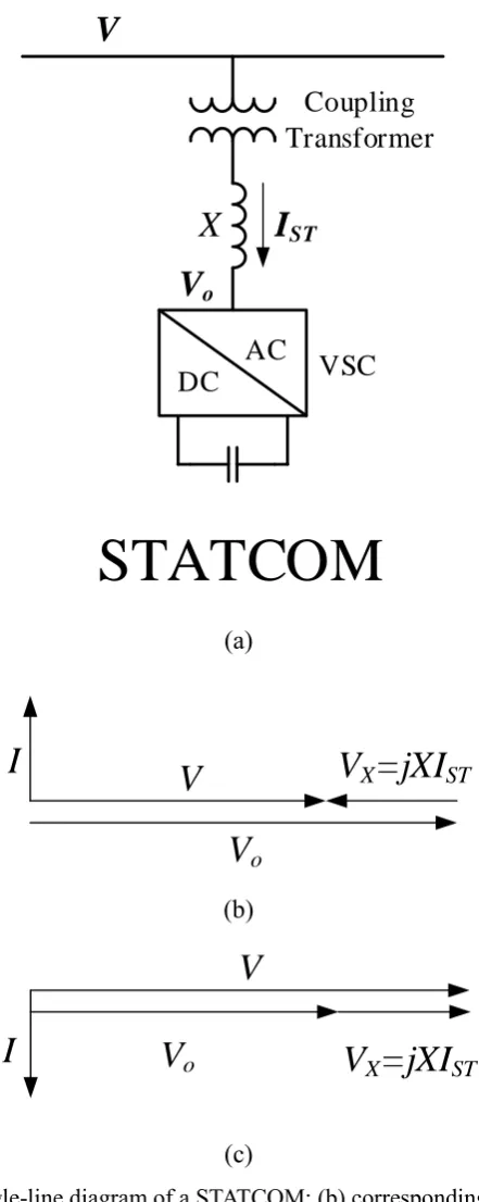
3.4.2 Static Synchronous Compensator ... 32
3.4.3 Static Synchronous Series Compensator ... 34
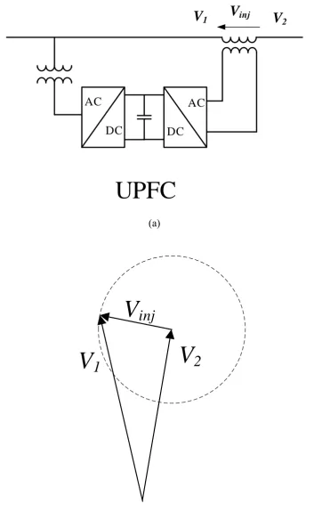
3.4.4 Unified Power Flow Controller ... 36
3.5 BACK-TO-BACK VOLTAGE SOURCE CONVERTER ... 38
3.6 RESEARCH ON USING POWER ELECTRONICS IN DISTRIBUTION NETWORKS... 38
3.7 SUMMARY ... 40
4.COMPENSATING DISTRIBUTION NETWORKS BY MESHING THE NETWORK ... 42
4.1 SOFT-OPEN POINTS ... 43
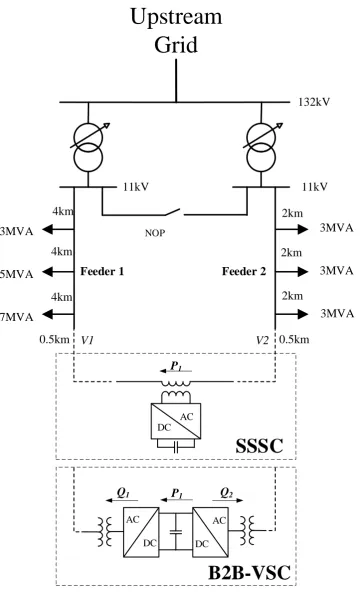
4.2 COMPARISON BETWEEN SSSC AND B2B-VSC ... 46
4.3 SUMMARY ... 54
5.CONTROLLER DESIGN OF A B2B-VSC BASED ON PROPORTIONAL-INTEGRAL THEORY ... 56
5.1 CONTROLLER DESIGN ... 56
5.1.1 Overall Structure of the Control System ... 56
5.1.2 Direct-quadrature-zero Transformation and Phase-locked Loop ... 57
5.1.3 Current Controller ... 62
5.1.4 DC Link Voltage Controller ... 66
5.1.5 Output Voltage Controller ... 73
5.2 SIMULATION RESULTS ... 79
iii
5.2.2 Fault Current Restriction ... 84
5.2.3 Loss of Mains ... 86
5.3 EXPERIMENT RESULTS ... 90
5.4 SUMMARY ... 94
6.CONTROLLER DESIGN OF B2B-SYNCHRONVERTER ... 96
6.1 SYNCHRONVERTER CONTROLLER ... 97
6.2 B2B-SYNCHRONVERTER CONTROLLER ... 104
6.3 SIMULATION RESULTS ... 109
6.3.1 Power Control and Voltage Compensation ... 111
6.3.2 Load Supply in Islanded Condition ... 115
6.3.3 Fault Current Limit ... 119
6.4 EXPERIMENT RESULTS ... 121
6.5 SUMMARY ... 124
7.SUPPLYING A NETWORK DOMINATED BY DYNAMIC LOAD VIA A VSC .. 126
7.1 AN INDUCTION MOTOR DURING A FAULT AT THE STATOR SIDE ... 126
7.2 STABILITY MARGIN OF AN INDUCTION MACHINE ... 130
7.3 CONTROLLING THE OUTPUT IMPEDANCE OF A VSC ... 138
7.4 SIMULATION RESULTS ... 143
7.5 EXPERIMENT RESULTS ... 147
7.6 SUMMARY ... 152
8.CONCLUSIONS AND FUTURE WORK ... 153
8.1 CONCLUSIONS ... 153
8.2 FUTURE WORK ... 156
BIBLIOGRAPHY ... 158
APPENDIX I ... 166
APPENDIX II ... 167
v
List of Figures
Figure 1.1 Electric power system [2]. ... 2
Figure 1.2 Types of fuel used for CHP in the UK in 2017. ... 5
Figure 1.3 UK electricity supply since 1980 [19]. ... 6
Figure 1.4. Electricity generation by fuel types in the UK in 2017. ... 7
Figure 1.5 Electricity generation by main renewable sources in the UK [20]. ... 7
Figure 2.1 (a) Power flow in distribution network; (b) Corresponding phasor diagram. ... 11
Figure 2.2 Studied 11kV distribution network ... 14
Figure 2.3 Breaking fault level increase with increasing DG Penetration level ... 15
Figure 2.4 Voltage increase with increasing DG penetration level ... 17
Figure 3.1 (a) Single-line diagram of two-machine power system; (b) Corresponding phasor diagram. ... 19
Figure 3.2 (a) Single-line diagram of shunt capacitor compensation for radial system; (b) corresponding phasor diagram. ... 22
Figure 3.3 (a) Single-line diagram of shunt reactor compensation for radial system; (b) corresponding phasor diagram. ... 23
Figure 3.4 (a) Single-line diagram of ideal mid-point shunt compensation for two-machine system; (b) Corresponding phasor diagram. ... 25
Figure 3.5 (a) Single-line diagram of series capacitor compensation for radial system; (b) corresponding phasor diagram. ... 26
Figure 3.6 (a) Single-line diagram of series reactor compensation for radial system; (b) corresponding phasor diagram. ... 27
Figure 3.7 (a) Single-line diagram of series capacitive compensation; (b) corresponding phasor diagram. ... 29
Figure 3.8 Single-line diagram of shunt compensators: TCR, TSC, FC-TCR and TSC-TCR. ... 31
Figure 3.9 Single-line diagram of series compensators: TSSC, TCSC, TCSR ... 31
vi
in capacitive compensation mode; (c) corresponding phase diagram in inductive
compensation mode. ... 33
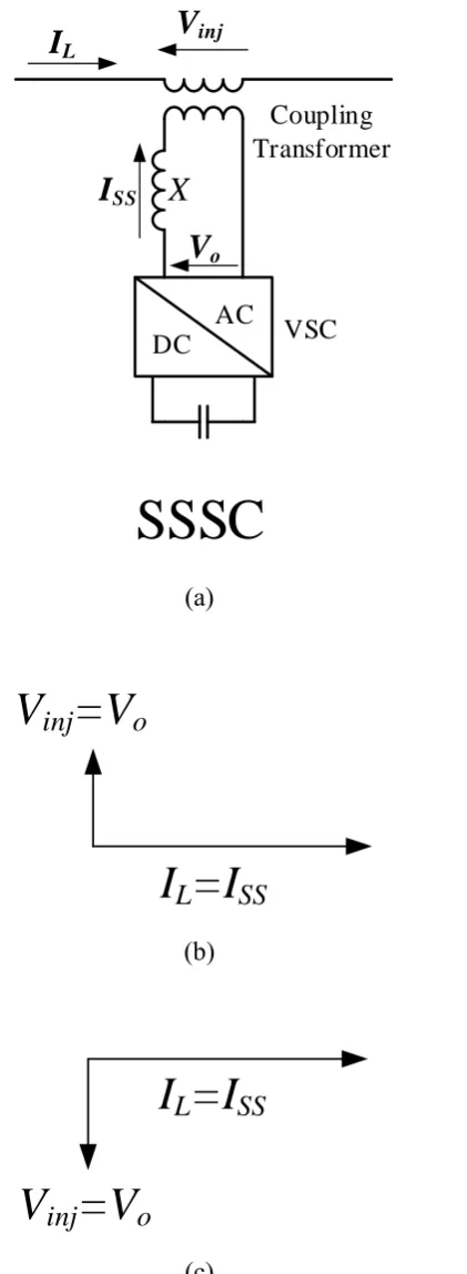
Figure 3.12 (a) Single-line diagram of a SSSC; (b) corresponding phasor diagram in capacitive compensation mode; (c) corresponding phasor diagram in inductive compensation mode. ... 35
Figure 3.13 (a) Single-line diagram of a unified power flow controller; (b) phasor diagram of voltage compensation capability ... 37
Figure 3.14 Back-to-back voltage source converter ... 38
Figure 4.1 A brief single-line diagram of two adjacent distribution networks built in meshed but operated in radial. ... 45
Figure 4.2 Single-line diagram of the studied network and SOP connections ... 47
Figure 4.3 Reactive power compensation by STATCOM: (a) Phase-to-ground voltage in per unit before and after compensation; (b) Power coming out from the supply transformer to Feeder 1. ... 49
Figure 4.4 Active and reactive power compensation by SSSC and B2B-VSC: (a) The voltages at feeder endpoints before and after compensation shown in per unit; (b) Power fed to Feeder 1 and Feeder 2 with B2B-VSC; (c) Power fed to Feeder 1 and Feeder 2 with SSSC. ... 51
Figure 4.5 Flow chart of power loss calculation ... 53
Figure 4.6 (a) Power loss of the B2B-VSC; (b) Power loss of the SSSC. ... 54
Figure 5.1 Controller diagram for the B2B-VSC. ... 57
Figure 5.2 Reference frame layouts used in this thesis ... 60
Figure 5.3 (a) Phase-locked loop; (b) Equivalent diagram for the Phase-locked loop. . 61
Figure 5.4 Full block diagram of the current control loop. ... 65
Figure 5.5 block diagram of DC link voltage loop ... 68
Figure 5.6 (a) Bode diagram at different tr; (b) Step responses at different tr. ... 72
Figure 5.7 Block diagram of output voltage control loop ... 74
Figure 5.8 State-space representation of output voltage control loop ... 76
Figure 5.9 Pole-zero map of the whole system at different rising time ... 77
Figure 5.10 Magnitude diagram from inputs u1, u2, u3 and u4 to output y1. ... 78
vii
Figure 5.12 Single-line diagram of studied network ... 79
Figure 5.13 (a) Output power of VSC1; (b) Output power of VSC2. ... 82
Figure 5.14 Phase voltage at endpoints of Feeder 1 and Feeder 2 in per unit. ... 82
Figure 5.15 DC link voltage ... 83
Figure 5.16 Output voltage and current of VSC1 ... 84
Figure 5.17 (a) Three-phase output voltages and inductor currents of VSC1 during fault; (b) Three-phase output voltages and inductor currents of VSC2 during fault. ... 85
Figure 5.18 Phase-a current at the fault point with B2B-VSC and NCP ... 86
Figure 5.19 Three-phase voltages and currents during loss of mains. ... 88
Figure 5.20 Amplitude in per unit of endpoints voltages V1 and V2. ... 88
Figure 5.21 Three-phase voltages and currents during loss of mains without reset in the output voltage controller. ... 89
Figure 5.22 Voltage and current responses during a load change. ... 90
Figure 5.23 Experiment Setup: (a) Experiment circuit; (b) Experiment facilities. ... 91
Figure 5.24 Three-phase voltages and currents at the load (a) Simulation result; (b) Experiment result. ... 93
Figure 5.25 Voltage and current in SRF during the loss of mains for the comparison between experiment and simulation results. ... 93
Figure 5.26 Output voltage and current of the VSC. ... 94
Figure 6.1 Simplified synchronous generator model ... 98
Figure 6.2 A VSC with an LC filter ... 101
Figure 6.3 Controller for one side of the B2B-synchronverter ... 103
Figure 6.4 Single-line diagram of the network setup. ... 110
Figure 6.5 Simulation results for power control and voltage compensation: (a) Output power of the synchronverter at Feeder 1; (b) Output power of the synchronverter at Feeder 2; (c) Voltage amplitude at endpoint of Feeder 1 in per unit; (d) Voltage amplitude at endpoint of Feeder 2 in per unit; (e) DC link voltage in volt. ... 114
Figure 6.6 Three-phase output voltage and current of the synchronverter at Feeder 1. ... 115 Figure 6.7 Simulation results for loss of mains: (a) Voltage amplitude at endpoint of
viii
synchronverter1; (d) Grid frequency at Feeder 2; (e) Output power of the synchronverter at
Feeder 1; (f) Output power of the synchronverter at Feeder 2. ... 117 Figure 6.8 DC link voltage during the loss of mains. ... 119 Figure 6.9 Three-phase output voltage and current of synchronverter1. ... 119 Figure 6.10 Output voltages and inductor currents during a three-phase-to-ground fault at Feeder: (a) Voltage and current of synchronverter 1; (b) Voltage and current of
synchronverter2. ... 120 Figure 6.11 Comparison between fault current (phase a) with B2B-synchronverter and with direct line/cable connection. ... 121
Figure 6.12 Experiment results during an islanding case: (a) Load voltage amplitude; (b) Frequency response; (c) Partially enlarged plot of the frequency; (d) Output power . ... 123
Figure 6.13 Three-phase voltage and current at the load. ... 124 Figure 7.1 Single-line diagram of an induction motor supplied by the mains via a variac. ... 127 Figure 7.2 Per-phase equivalent circuit when the stator side is short-circuited. ... 127 Figure 7.3 Simulation of effects of a fault to an induction motor: (a) Three-phase voltage and current at stator; (b) Active and reactive power flowing in the motor; (c) Rotor flux; (d) Rotor speed. ... 130
Figure 7.4 Single-line diagram of an induction motor supplied by the mains via a variac. ... 131 Figure 7.5 Per-phase equivalent circuit of an induction motor ... 131 Figure 7.6 Thevenin equivalent of induction motor circuit (a) Thevenin voltage of the input circuit; (b) Thevenin impedance of the input circuit; (c) Whole Thevenin equivalent circuit... 133
Figure 7.7 Thevenin equivalent solution for an induction motor supplied by an VSC with LC filter: (a) original circuit; (b) Thevenin circuit for filter has been applied; (c) final Thevenin equivalent circuit for the whole circuit. ... 136
Figure 7.8 Toque-speed characteristics ... 138 Figure 7.9 (a) Single-line diagram of a VSC with LC filter; (b) Corresponding block diagram. ... 139
ix
Figure 7.11 Output voltage control loop by neglecting coupling and decoupling ... 140 Figure 7.12 Bode diagrams of Z1(s) when G(s)=0, G(s)=1 and for proposed G(s). .... 142
Figure 7.13 Bode diagram of proposed G and τs+1 ... 143 Figure 7.14 Torque-speed characteristic at 95V line voltage when connected to grid and open-loop controlled VSC. ... 144
Figure 7.15 Simulation results of power supply to an induction motor by a VSC in island mode including the islanding transition: (a) Output three-phase voltage and current of the VSC; (b) Output active and reactive power of the VSC; (c) Rotor speed of the induction motor. ... 145
Figure 7.16 Simulation results when the VSC is open-loop controlled: (a) Output voltage and current of the VSC; (b) Rotor speed of the induction motor. ... 146
Figure 7.17 Experiment Setup: (a) single-line diagram of the experiment setup; (b) photos of equipment. ... 148
Figure 7.18 Experiment result during the loss of mains when the VSC is in the proposed closed-loop control: (a) Output three-phase voltage and current of the VSC; (b) Output active and reactive power of the VSC; (c) Torque on the rotor shaft and rotor speed... 150
x
List of Tables
Table 1-1 Recent development of CHP in the UK ... 4
Table 1-2 CHP schemes by capacity size ranges in the UK in 2017 ... 5
Table 5-1 The maximum overshoots at different damping ratios ... 71
Table 5-2 Used parameters ... 71
Table 5-3 System parameters ... 80
Table 5-4 Events in voltage compensation simulation ... 81
Table 5-5 Events in loss of mains simulation ... 87
Table 5-6 Parameters in experiment ... 92
Table 6-1 Simulation Parameters ... 111
Table 6-2 Operation scenarios in simulation ... 112
Table 6-3 Experiment Parameters ... 122
Table 7-1 Parameters of the induction motor and VSC’s filter ... 128
xi
Acknowledgement
I would like to present my sincerely thanks to all people and organisations who offered help and supports to me during my PhD study. Among them, there are some persons I would like to present my thankfulness individually.
First and foremost, I would like to present my most gratefully and sincerely thanks to my supervisor, Professor Li Ran, for all his help, encouragement, guidance and care during my whole PhD study in the University of Warwick. I have been extremely lucky to have a supervisor who cared so much about my work and life; who taught me a lot about academics and researches; and who spent so much time and effort to revise my papers.
I would also like to thank Dr. James Yu for offering me the opportunity to participate in the Offshore Low Frequency ac Power Transmission project. I am especially grateful for the scholarship and support from James.
I would like to thank the Technician Team in the school of Engineering for supporting my researches. I would like to thank Ian Griffith, Gavin Downs and especially Jonathan Meadows for helping build the test platform for the induction machine research and of course for other experiment setup. I would also like to thank Jose Ortiz Gonzalez for helping me on experiments with his rich experience.
I would like to thank my colleague Tianqu Hao for guiding me use dSpace for experiments. I would like to thank Han Qin, Erfan Bashar and Weihua Shao for the great time that we wrote papers together. I would also like to thank all my other friends and colleagues: Yuan Tang, Ji Hu, Fan Li, Tianxiang Dai, Xuan Guo, Roozbeh Bonyadi, Saeed, Ben, Guy for their support and the happy memories on dinners, drinks, jokes and football games!
xii
Declaration
The work presented in this thesis is based on research carried out by the candidate in the School of Engineering, the University of Warwick, UK. No part of this thesis has been submitted for any other degree or qualifications at any other university. Part of the work presented in Chapter 2 has been published in C1 (list of publication is in Appendix III). Part of the work presented in Chapter 4 has been published in C2. C1 and C2 are based on collaborative researches and the contents presented in this thesis are contributed by the candidate. The work presented in Chapter 6 has been published in J1.
Ruizhu Wu
xiii
Abstract
xiv
Abbreviation
AC alternating current DC direct current
NGET National Grid Electricity Transmission plc DNOs Distribution Network Operators
DG distributed generation CHP combined heat and power SOP Soft-open point
NOP normally-open point VSC voltage source converter B2B back-to-back
FL fault level
VLnom nominal line voltage
If fault current
rms root-mean-square p.u. per unit
OLTC on-load tap changer
RL resistance of a power line
XL reactance of a power line
XC capacitor reactance
Xre reactor reactance
FACTS Flexible AC Transmission System SVC static VAR compensator
TCR Thyristor-Controlled Reactor TSR Thyristor-Switched Reactor TSC Thyristor-Switched Capacitor
FC-TCR Fixed Capacitor Thyristor-Controlled Reactor
TSC-TCR Thyristor-Switched Capacitor-Thyristor-Controlled Reactor TSSC Thyristor-Switched Series Capacitor
TCSC Thyristor-Controlled Series Capacitor TCSR Thyristor-Controlled Series Reactor STATCOM static synchronous compensator GTO Gate Turn-Off Thyristor
IGBT Integrated Gate Bipolar Transistor MTO MOS Turn-off Thyristor
IGCT Integrated Gate-commutated Thyristor SSSC static synchronous series compensator
Vinj Injected voltage to the network by a compensator
UPFC unified power flow controller HVDC High-voltage direct current
Vs sending voltage
Vr receiving voltage
xv
R general resistance
X general reactance
P active power
Q reactive power
PL load demand power
PDG output power by DG
Vce voltage between collector and emitter
Ic collector current
Etotal total energy loss of a device
eon device’s turn-on loss
eoff device’s turn-off loss
erec diode’s reverse recovery loss
PR proportion-resonant PI proportional-integral
Rf filter resistance
Lf filter inductance
Cf filter capacitance
vi phase voltage before filter
vo output phase voltage
iL filter inductor current
io output current
ic capacitor current
ω angular velocity
vDC DC link voltage
Xabc balanced three-phase quantities
X* reference value to a quantity
Xd quantity at d axis
Xq quantity at q axis
Xdq Xdq=Xd+jXq
Xα quantity at α axis
Xβ quantity at β axis
Xαβ Xαβ=Xα+jXβ
dq0 direct-quadrature-zero SRF synchronous reference frame
Kc amplitude-invariant Clark transformation matrix
Kp Park transformation matrix
T[θ] dq0 transformation matrix
T-1[θ] inverse dq0 transformation matrix
Vm voltage amplitude
θ0 angle of reference voltage
θ angle of controlled voltage PLL phase-locked loop
GPLL(s) phase-locked loop controller
KP_PLL PLL controller proportional gain
KI_PLL PLL controller integral gain
xvi
ξPLL PLL damping ratio
KP_C current controller proportional gain
KI_C current controller integral gain
Td total delay in VSC process
fs PWM sampling and converter switching frequency
Ts PWM sampling time Ts=1/fs 𝑒−(𝑠+𝑗𝜔)𝑇𝑑 total delay in SRF
𝑒𝑗𝜔𝑇𝑑 delay compensation term in SRF GC(s) current controller gain
HC(s) current loop plant
GCL(s) current loop closed-loop transfer function 𝐿̂𝑓 estimations of the filter inductance
𝑅̂𝑓 estimations of the filter resistance
τ current loop time constant
n n=1/ τ
PDC power flowing into or out from the DC link
u square of the DC link voltage
U(s) square of the DC link voltage is s domain
C DC link capacitance
GDC(s) DC link voltage controller gain
HDC(s) DC link voltage plant transfer function
KP_DC DC link voltage controller proportional gain
KI_DC DC link voltage controller integral gain
NDCVL(s) open-loop transfer function of DC link voltage loop
GDCVL(s) closed-loop transfer function of DC link voltage loop
G’DCVL(s) simplified closed-loop transfer function of DC link voltage loop
ωDC DC link voltage control loop natural frequency
ξDC DC link voltage control loop damping ratio
ωn arbitrary natural frequency of a second-order system or nominal angular
velocity
ξ arbitrary damping ratio of a second-order system
𝜔𝑑 𝜔𝑑 = 𝜔𝑛√1 − 𝜉2 (0 < 𝜉 < 1)
Hstep(s) step response in s domain
hstep(t) step response in time domain
tp time required to reach the first peak
hpeak Peak value of the overshoot
Mp Maximum overshoot
tr rising time of second-order systems
HV(s) transfer function of output voltage loop
GV(s) output voltage controller gain
KP_V output voltage controller proportional gain
KI_V output voltage controller integral gain
G’VL(s) simplified closed-loop transfer function of output voltage loop
ωV output voltage control loop natural frequency
xvii
tr_V rising time of output voltage control loop
u1 input 1 of the state-space matrices of output voltage control loop
u2 input 2 of the state-space matrices of output voltage control loop
u3 input 3 of the state-space matrices of output voltage control loop
u4 input 4 of the state-space matrices of output voltage control loop
y1 output 1 of the state-space matrices of output voltage control loop
y2 output 2 of the state-space matrices of output voltage control loop
X1 quantities at or connected to Feeder 1
X2 quantities at or connected to Feeder 2
PF power factor
THD total harmonic distortion variac variable transformer
Rs stator resistance
Ls stator inductance
M mutual inductance between two stator phase windings across the air-gap and a round rotor
𝑀𝑎𝑟,
𝑀𝑏𝑟, 𝑀𝑐𝑟
mutual inductances between each stator phase and the rotor excitation winding
ir rotor excitation current
𝜆 flux linkages
vin induced voltage in a synchronous machine
e voltage induced by rotor current
J inertia of the rotor
Tm mechanical torque
Te electromagnetic torque
K control gain of Q-V loop
Pm actually the electric power exchanged with the DC link
Pe output electric power to the AC terminal
DP_t angular velocity damping factor
DP 𝐷𝑃= 𝜔 ∙ 𝐷𝑃_𝑡
Dq droop gain of Q-V loop
τ1 time constant of P-ω loop
τ2 time constant of Q-V loop
ωg grid angular velocity
Kp proportional gain of PI controller in P-ω loop
Ki integral gain of PI controller in P-ω loop
KDC control gain of DC link voltage controller
LM magnetizing inductance
XM magnetizing reactance
Lr referred rotor inductance
Xr referred rotor reactance
Rr referred rotor resistance
Xs stator reactance
s slip
Ir rotor current
xviii
nm mechanical shaft speed
T induced toque in an induction machine
Pag air-gap power
ωsync synchronous angular velocity
Vth Thevenin equivalent voltage
Zth Thevenin equivalent impedance
Rth Thevenin equivalent resistance
Xth Thevenin equivalent reactance
XLf filter reactance by the inductor
XCf filter reactance by the capacitor
Vfth Thevenin equivalent voltage for VSC filter
Zfth Thevenin equivalent impedance for VSC filter
Rfth Thevenin equivalent resistance for VSC filter
Xfth Thevenin equivalent reactance for VSC filter
ωLF cut-off frequency of the low pass filter
G(s) current feedforward gain
1
1.Introduction
1.1
Conventional Electric Power System
Electric power systems have been formed by centralised power stations, transmission systems and distribution networks for over several decades. However, in early days of electricity, power stations were constructed in the adjacent of customers and relatively simple networks were built to connect them. Then, this scheme was replaced by the unified electricity grid due to the rapid increase of power demand. In Great Britain, the ‘national grid’ was first established in 1930. Those simple networks built in the early days were converted to distribution networks. Following by a rapid development period in the 1950s and 1960s, the National Supergrid system in the United Kingdom today was formed [1].
In today’s electric systems the majority of electric power is generated in large power stations in three-phase form to achieve constant power generation and defined as the product of two quantities: AC current and AC voltage. Then the power is stepped up to high voltage level by transformers and then carried by the transmission systems from generating centres to load centres. Approximately 85% of the total generating capacity in the UK is connected to the national transmission system which is operated by National Grid Electricity Transmission plc (NGET). At downstream system are distribution networks, operated by Distribution Network Operators (DNOs), by which the power is stepped down to medium and low voltage levels and fed to customers such as residences, hospitals and industries. Figure 1.1 shows a brief figure for the conventional electric power system.
2
Figure 1.1 Electric power system [2].
With the rapidly increasing consumption of electricity, the reserves of fossil fuels will be greatly consumed in the near future. The exhaustion of oil and gas could happen in a century and the exhaustion of coal could happen in two or three centuries [3, 4]. Besides, although electricity has been providing great development and convenience to human beings, the generation of it causes pollutions to environment. Therefore, to seek cleaner and more sufficient electricity generation becomes an inevitable demand throughout the world.
1.2
Distributed Generation
Distributed generation (DG), also known as embedded generation or on-site generation or dispersed generation, can be described as the generation of electricity from decentralized and small-scale generators which are mostly placed at load centres. DG units are connected to distribution networks rather than the transmission network [5-11]. It is more flexible than centralized power generation and has very low power loss in transmission as they are located in the vicinity of customers [6, 12]. Compared to conventional power system, a highly distributed system could provide benefits such as:
3
• Higher efficiency – lower power loss in transmission and CHP is a more efficient way of utilising primary fuels;
• Improved flexibility and reliability – modular and decentralised system might be able to operate individually to secure local demand and adapt more readily to technology changes;
• More competition in the market – a decentralised system encourages more participants thus increasing competition [1].
In the past, distributed generation refers to combustion generators which is not clean. In recent years, renewable resources particularly wind and solar energy have been greatly developed as the distributed generation. Under the megatrends of low carbon footprints, it is expected that the distributed generation of renewable resources will play an important role in the future electric power system. The following part of this section will summarise the statistics of main types of distributed generation in the UK in recent years to illustrate the development trend.
1.2.1
Combined Heat and Power
Combined heat and power (CHP) or cogeneration is the simultaneous generation of electricity and useful heat. CHP is not necessarily low-carbon but is definitely more efficient than generating electricity and heat separately. The overall efficiency of the energy conversion of a CHP plant can be over 80% which is approximately 1.6 times of the efficiency of a good combined cycle gas turbine station [13]. CHP was used in manufacturing industry in the early days and the first installation was probably in Glasgow in 1898. In 1980s, CHP-based district heating, which is to district the heat generated in power stations to local buildings, was greatly developed by the support from government in the UK [14]. In 1990s, the UK’s first major modern heat-distribution grid was built in Sheffield, and small-scale CHPs were being developed [15].
4
generated in the UK. The overall efficiencies are always over 70% thanks to the UK’s CHP Quality Assurance programme which requires a Good Quality CHP scheme over 1 MWe must achieve 10% primary energy savings compared to separate generation of heat and power.
Table 1-1 Recent development of CHP in the UK
Unit 2013 2014 2015 2016 2017 Number of schemes 2024 2017 2130 2224 2386 Electrical capacity MWe(1) 5919 5888 5708 5625 5835 Heat capacity MWth(2) 22161 22223 20091 19795 20191 Fuel input GWh 88403 86184 82576 85123 90279 Electricity generation GWh 19515 19690 19534 20405 21648 Heat generation GWh 44342 41950 40234 40670 42238 Overall efficiency Per cent 72.2 71.5 72.4 71.7 70.8
(1) MWe: Megawatt electric. (2) MWth: Megawatt thermal.
In general, CHP plants can be divided into three levels depending on the size [17]:
• Micro CHP plants for domestic use generating both electricity and heat for the home;
• Medium CHP plants generating both electricity and heat for a whole building or community area;
• Large CHP plants generating heat for local use and electricity that fed into high voltage distribution network or even transmission network.
A statistic of CHP by capacity size in 2017 is shown in Table 1-1. Micro and Medium CHP plants are dominant in numbers (over 80%), but large CHP plants output the majority of electricity (72%). It is worth noting that, from the electricity generation point of view, some of the large CHP plants should not be counted as distributed generation because though the heat generated is used locally, the electricity generated is fed into transmission networks rather than distribution networks.
5
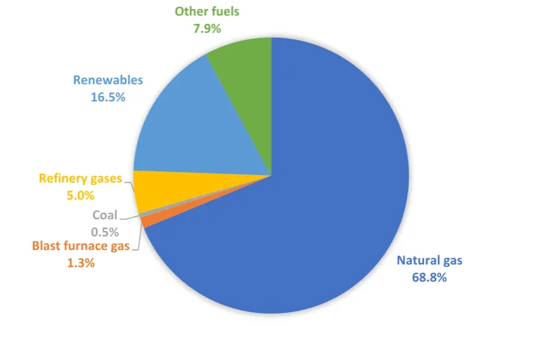
the renewable fuel consumption increased from 13% in 2016 to 16.5% in 2017.
Table 1-2 CHP schemes by capacity size ranges in the UK in 2017
Electrical capacity size range
Number of schemes and share of total
Total electricity capacity (MWe) and share of total <100kWe 605 (25%) 36 (0.6%)
100kWe ~ 1MWe 1291 (54%) 331 (5.7%) 1MWe ~ 2MWe 183 (7.7%) 259 (4.4%) 2MWe ~ 10MWe 240 (10%) 1027 (18%) >10MWe 67 (2.8%) 4181 (72%)
[image:25.595.139.529.386.631.2]Total 2386 5835
Figure 1.2 Types of fuel used for CHP in the UK in 2017.
1.2.2
Renewable Energies
Renewable energy is the energy from renewable resources which are naturally
Natural gas 68.8% Blast furnace gas
1.3% Coal 0.5%
Refinery gases 5.0%
Renewables 16.5%
6
replenished on a human timescale such as wind, sunlight and tides. Renewable energies are not new to human society. In fact, human beings started to use traditional biomass to fuel fires about 790,000 years ago [18]. However, the electricity generation by renewable energies has only been developed and implemented in recent decades.
The development of electricity supply in the UK since 1980 is shown in Figure 1.3 [19]. Electricity supply is fully driven by demand. The demand for electricity has been dropping because of the improving energy efficiency and overall warmer weather in the UK. However, the proportion of renewables has been greatly increased, trebled in 2017 compared to 2010. On the contrary, the use of fossil fuels has seen a large reduction since 2010, 44% reduction from 2010 to 2017. These changes on electricity supply in the UK are due to a continuation of the shift in fuel mix away from coal [19].
Figure 1.3 UK electricity supply since 1980 [19].
In terms of the share of electricity generation by renewable energies, wind occupied half of the electricity generation, 29% and 21% by onshore and offshore respectively in the UK in 2017 as shown in Figure 1.4. The proportion of the electricity generated by renewable sources to the total electricity generation is 29.3% (99.3 TWh) in the UK in 2017, was 24.5% (83.1-TWh) in 2016 [20]. A long-term trend of electricity generation by renewable sources is shown in Figure 1.5. From 2010, renewable energies have been greatly exploited where wind and solar share the major proportion of the increase of electricity generation.
7
[image:27.595.155.467.165.375.2]windfarms are usually connected to transmission network. However, it still shows a promising trend of the increasing DG from renewable sources.
Figure 1.4. Electricity generation by fuel types in the UK in 2017.
Figure 1.5 Electricity generation by main renewable sources in the UK [20].
Onshore wind 29%
Offshore wind 21% Solar PV
12%
Landfill gas 4%
Other bioenergy
28%
[image:27.595.120.543.438.680.2]8
1.3
Next Generation of Power Grid
The smart grid or known as the intelligent/micro grid is a promising trend of the future power grid. The smart grid combines a large amount of renewable energy resources that are distributed in the adjacent of customers. The smart grid in principle can run alone in islanded mode or have power exchange with the whole power grid depending on different scenarios. In comparison with the conventional power system, the main advantages of the smart grid include cleaner resources, higher power efficiency and reliability, faster response and can be thoroughly controlled [21-26]. However, in order to achieve that, sensors are required throughout the network and lacking large inertia could be a potential risk for the system’s stability [27, 28]. More importantly, most of the renewable energy resources are inherently intermittent which could cause serious problems in extreme cases.
The smart grid system cannot be built in one day. There must be a gradual and sustained development for the electric power system to evolve to the next generation. To install increasing number of DG to the existing distribution networks is in the way of the system’s evolution [29]. To address issues introduced by the integration of DGs will help us improve the network performance and have a better understanding of the future power system.
In this thesis, the issues introduced by increasing DGs are firstly analysed. Then, solutions by using power-electronic converters and associated control systems are proposed and studied.
1.4
Outline of the Thesis
In Chapter 1, the history of the electric power system is briefly introduced and a trend of increasing renewable DG in distribution networks in the UK is showed based on the historical statistics from government reports.
9
In Chapter 3, popular compensating technologies that normally used in transmission system are reviewed to seek solutions to the problem raised in Chapter 2.
In Chapter 4, the idea of a soft-open point (SOP) is introduced: using power-electronic based devices (reviewed in Chapter 3) to replace a normally-open point (refer to conventional circuit breaker) to gain advantages of meshed networks. Comparisons between the SSSC-based SOP as the most simple and economic option and the B2B-VSC-based SOP as the most versatile option are made by simulation. The B2B-VSC is preferred to be selected to be implemented to improve the network flexibility because of its capability of restricting fault current
In Chapter 5, the controller of a B2B-VSC based on proportional-integral (PI) theory is developed including detailed analyses on parameter design. The importance of resetting an integrator in the controller to achieve smooth transition from grid-connected mode to island mode is proposed. The controller is validated fully by simulation and partially by experiment.
In Chapter 6, a synchronverter-based controller for the B2B-VSC is developed which makes the converters behave like synchronous machines thus can automatically work in both grid-connected mode and island mode. It requires less detections and logic switches in controller compared to the controller built in Chapter 5, and offers better performance in islanding transition. The controller is validated fully by simulation and partially by experiment.
In Chapter 7, the use of an SOP in network dominated by dynamic load is investigated. The focus is on the influence of a fault and the loss of mains on a dynamic load, i.e. an induction motor. How the stability margin of an induction motor is affected by the filter impedance of a voltage source converter is analysed using the torque-speed characteristic. A controller reducing the VSC’s output impedance is proposed and validated by simulation and experiment.
10
2.Issues of Distribution Networks with High
DG Penetration Level
2.1
DG Penetration Level
DG penetration level is the ratio of the total capacity of DG to the total capacity of load in a distribution network. Although DG has been widely researched and used in the world [30], the DG penetration level is still low because the integration of DG could pose problems regarding the voltage profile, the fault current and the operational stability [31-35]. Especially for DGs powered by wind and solar energies, the inherent intermittency and seasonal variations pose more challenges [36-38]. The power systems we have today are built on the basis that the power flow is unidirectional from the upstream (generating centres) to downstream (end users) via transmission and distribution networks. However, with the integration of DG the power flow in the grid will be affected and could be reversed to flow from downstream to upstream in some situations. The new pattern of power flow will pose great challenges to the existing power system. Furthermore, the inherent intermittency of the DG using wind and solar energies increases the difficulty to manage the system.
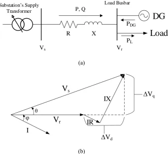
In electric power systems, losses of power and voltage are caused by the impedance of transmission lines and power lines/cables. Figure 2.1 shows a brief single-line diagram of a distribution network and its corresponding vector diagram of voltages and current. For a conventional distribution network, active and reactive power are transmitted from the substation in the upstream to load in the downstream via power lines/cables with electric impedance in all circumstances. As shown in Figure 2.1 (a), Vs and Vrare the phase voltages
at sending and receiving ends, I is current flowing in the power line/cable, φ is the phase ang between I and Vr, R and X are the electric resistance and reactance of the power line/cable,
11
Vs Vr
R X
DG
Load
PDG
Substation s Supply
Transformer P, Q
PL Load Busbar (a)
I
IR
IX
V
rV
s θᵠ
V
dV
q (b)Figure 2.1 (a) Power flow in distribution network; (b) Corresponding phasor diagram.
The derivative is shown as
(
)
(
) (
)
2 2 2 2 2 2 2cos sin cos sin
s r d q
r r
r r r r
V V V V
V RI XI XI RI
PR QX PX QR
V
V V V V
= + + = + + + − = + + + − (2.1) where d r PR QX V V +
= and q
r
PX QR
V
V
−
[image:31.595.167.509.107.420.2]12 If and normally,
r d q
V + V V (2.3)
then equation (2.1) can be rewritten as
s r
r
PR QX
V V
V +
= + . (2.4)
Therefore, the arithmetic difference between the sending and receiving voltages, that is the voltage drop, can be approximately expressed as
r
PR QX V
V +
= . (2.5)
Because of the low X/R ratio of cables and the generally high load power factor in distribution networks, it is reasonable to simplify equation (2.5) as
r
PR V
V
= (2.6)
which indicates that the voltage drop is dominantly affected by the active power flow. In a distribution network with DG, the active power passing the cable should be the active power consumed by the load minus the active power generated by DG which is represented by P=PL -PDG. This explains that the lower voltage drops and power loss on
lines/cables can be achieved as DG shares the load demand. However, the power could flow reversely from downstream to upstream if the DG outputs excessive power to the load demand which could cause a voltage rise at load busbar.
13
level, i.e. 100% penetration level - DG capacity equals load capacity, the voltage could rise beyond the permitted boundary which is called a voltage violation. Furthermore, high DG penetration level could also result in the fault current exceeding the making/breaking duties of circuit breakers as there are more sources contributing fault current. The following two sections investigate two major issues, fault level increase and voltage violation, in a distribution network with high DG penetration level by simulation using reasonable parameters.
2.2
Distribution Network Operating Regulations and Modelling
To investigate the influence of DG on the voltage profile and fault level in distribution networks, firstly a distribution network model needs to be built. In the UK, the supply transformers in substations step down the voltage from 132kV or 33kV to 11kV and feed the load demand which is typically about 10MVA ~ 20MVA (generally higher in urban area and lower in rural area) with an average power factor of about 0.97 in a radial distribution network. The loads are distributed along a feeder which has the length of about 5km ~ 10km (generally shorter in urban area and longer in rural area). The voltage must be within +6% ~ -6% of the nominal voltage which is set by DNOs in their operation [39]. The frequency must be within +1% ~ -1% of the nominal frequency which is 50Hz in the UK [40]. There are circuit breakers distributed in networks having the rating of typically 625MVA for make and 250MVA for break.
14
Substation Supply Transformer
Load
5MVA
Load
5MVA
Load
5MVA 3km Cable 3km Cable 3km Cable
DG Feeder
11kV Busbar
a b c
Figure 2.2 Studied 11kV distribution network
2.3
Fault Level Increase
The fault level is usually used, in the network design and operation, to represent the fault/short-circuit current in the unit of MVA. The three-phase fault level is defined as:
3 Lnom f
FL= V I (2.7)
where VLnom is the nominal line voltage and If is the fault current. A typical fault current in
the AC electric system consists of an AC component and a decaying DC component due to the inductive part of the system. Two terms, ‘make’ and ‘break’, are used to express the first peak value, and respectively, the root-mean-square (rms) value of the AC component of the fault current. The making and breaking capacities of the circuit breaker in 11kV distribution networks in the UK are typically 625MVA and 250MVA. Currently in the UK the average fault level of a 11kV distribution network is at about 70% of the capacity of the circuit breaker.
15 level on average.
In this study, the influence of DG on the fault level at the primary busbar as shown by the red zigzag arrow in Figure 2.2, which is the highest fault level point, is investigated. The DG is considered to be centrally located at position a, b, or c which is from close to far away from the substation to have a better understanding of how the location affects the fault level contribution. The type of all DG units is selected as synchronous machine for the worst case.
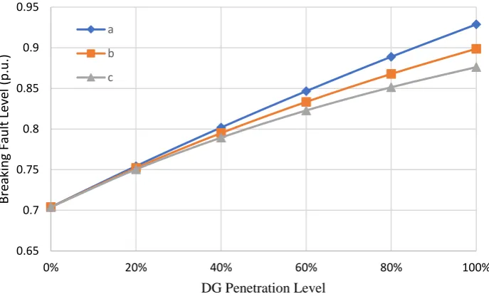
[image:35.595.162.506.397.607.2]The simulation result by Matlab/Simulink is shown in Figure 2.3. The per unit of breaking fault level (base is 250MVA) is shown with different penetration levels and locations of DG. In general, the higher DG penetration level contributes larger fault current and closer location results in higher fault level due to lower cable impedance. The largest fault level increase is observed at location a with 100% DG penetration level which makes the fault level to be 92.5% of the capacity of the circuit breaker. Considering the preservation of 5% safety margin in operation, it is very close to the upper limit which is 95%.
Figure 2.3 Breaking fault level increase with increasing DG Penetration level
2.4
Voltage Violation
The voltage violation means the voltage rises or drops outside the permitted range which is 0.94~1.06p.u. that adopted by UK DNOs in their operation. The majority of UK’s
0.65 0.7 0.75 0.8 0.85 0.9 0.95
0% 20% 40% 60% 80% 100%
B
re
ak
ing
Fau
lt
Le
ve
l (p.u
.)
DG Penetration Level a
b
16
distribution networks are built in meshed but operated in radial topology where a network is only supplied by one source from the distribution substation. The voltage at the end load busbar, location c in Figure 2.2, could drop considerably when the load demand is high as expressed by equation (2.6). Therefore, usually the output voltage at the substation is set higher than 1p.u. by positioning the on-load tap changer (OLTC) in the supply transformer to ensure the voltage at the end load busbar stays within the permitted range. A tap changer can have 16 taps for ±10% variation (each step providing 1.25% variation) from the nominal value. Tap changers are not operated dynamically because rapid changes can significantly reduce the lifetime. In this study, the voltage at the primary side is assumed at 0.9625p.u. (about 1.04p.u. at the secondary side) and the tap changer is remained at this position in all scenarios.
By integrating DG into the network, the voltage is expected to be increased because that less power from the substation experienced by the cable impedance. However, the voltage could rise beyond the upper limit when the network is lightly loaded. In an extreme case that the output of DG is at the maximum while the load demand is zero, voltage violation could occur. Figure 2.4 shows the simulation results of voltage rise in this extreme case with increasing DG penetration level at different locations. In general, higher DG penetration levels and farther locations result in higher voltage rises. The slowest voltage violation could happen when the DG penetration level increases to approximately 80% and the DG units are concentratedly placed at location a.
This is compliant with equation (2.6). In the extreme case, the load power PL is zero.
Thus, the power flowing through the feeder will be
L DG DG
P=P −P = −P . (2.8)
Then, by neglecting the QX, equation (2.4) can be rewritten as
DG r s
r
P R
V V
V
= + . (2.9)
17
[image:37.595.157.505.167.367.2]in higher voltage rise; similarly, for a certain location - fixed R, the higher DG penetration level - larger PDG results in higher voltage rise.
Figure 2.4 Voltage increase with increasing DG penetration level
2.5
Summary
In a distribution network, the voltage violation issue is likely to be met first when the DG penetration level increases. And UK DNOs in practice are inclined to allow very limited DG to be installed close to the primary busbar from the safety point of view. Therefore, the voltage violation would be a more common issue for building distribution networks with high DG penetration level. However, for networks already having high fault levels, the increase on the fault level should be treated prudently.
1.03 1.04 1.05 1.06 1.07 1.08 1.09 1.1
0% 20% 40% 60% 80% 100%
Vo
ltag
e
A
m
p
litu
d
e
(p
.u
.)
DG Penetration Level
a
b
c
18
3.Review of Compensating Devices
3.1
Active and Reactive Power
Before discussing the compensating devices, it is important to introduce the concept of active and reactive power first. In electric system, active power is easy to understand as it is the power that does the real work. It is determined by the voltage amplitude, current amplitude and the angle between them. For defined voltage and current, the smaller angle corresponds to higher power factor which results in higher active power and relatively lower reactive power, and vice versa. Reactive power is also an essential part of the electric system and is generated when the current is not in phase with the voltage due to inductive or capacitive components. It produces alternating magnetic fields in asynchronous motors and electrical transformers. Around 65% and 25% of the reactive power is used to produce alternating magnetic fields in asynchronous motors and electrical transformers. For industrial case, the weight is around 70% and 20% [42].
For a long radial overhead line in a transmission system, the voltage drop is mainly affected by the reactive power experienced by the transmission lines because of the high X/R
impedance ratio of the line. In fact, the resistance of transmission lines is usually negligible compared to the reactance [43]. Therefore, equation (2.5) can be written as
r
QX V
V
= (3.1)
which indicates that the reactive power is the main factor of the voltage drop for a long radial overhead line in transmission systems.
19
XL
V
sV
rI
(a)
(b)
Figure 3.1 (a) Single-line diagram of two-machine power system; (b) Corresponding phasor diagram.
The reactance of the transmission line is XL and the resistance is neglected. The sending
voltage Vs is leading the receiving voltage Vr by the angle θ. Assuming that Vs=Vr=V, the
angles between the current and the voltages Vs and Vr are -θ/2 and +θ/2, respectively. The
current can be calculated by:
2 sin
2
L L L
V V
I
X X
= = . (3.2)
Then, the active power and reactive power at the receiving end can be given as:
V
rV
sV
L=jIX
Lθ
20
2
sin
r L
V P
X
= (3.3)
and
(
)
2
1 cos
r L
V Q
X
= − . (3.4)
In the following sections of this chapter, technologies that have been developed to compensate the reactive power in transmission systems to achieve higher active power transmitted and better voltage profile will be introduced.
3.2
Conventional Compensators
In early years, reactive power compensation is carried out by large equipment such as capacitor banks, reactors or synchronous condensers.
3.2.1
Shunt and Series Capacitor
As the names imply, shunt and series capacitors are the capacitors connected in shunt and series with power lines, respectively. Parallel capacitors generate reactive power to increase the power factor thus increasing the active power capacity in transmission. Series capacitors create a negative reactance in power lines to reduce the active and reactive power consumption.
3.2.2
Reactor
Reactors in electric power system are usually used to consume excessive reactive power which functions as opposite to shunt capacitors. They are usually placed at the end of transmission lines or in substations to avoid overvoltage.
21
A synchronous condenser is a DC-excited synchronous motor which operates at no load condition. By controlling its excitation current, it can generate or absorb reactive power as required to improve the voltage profile and power factor. In under-excited condition, the synchronous condenser absorbs both active and reactive power from the network. And in over-excited condition, it draws active power but outputs reactive power to the network.
Compared to capacitor banks, synchronous condensers can be dynamically and continuously adjusted without steps and do not have switching transients. Besides, synchronous condensers are not affected by system harmonics or susceptible to resonances. However, the disadvantage of synchronous condensers is the relatively high power loss.
3.3
Basic Principles of Reactive Power Compensation
The reactive power compensation can be divided into shunt and series compensations from the aspect of connection type. There are also two types of system commonly used for analyses of compensation: the two-machine system and radial system. In two-machine systems, both the sending and receiving voltages are considered to be fixed which is usually used for transmission networks. In radial systems, only either the sending or receiving end voltage is considered to be fixed which is usually used for distribution networks or downstream sections of transmission networks. In this section, basic principles of shunt and series compensations are introduced including both capacitive and inductive types with the help of phasor diagrams.
3.3.1
Shunt Compensation
3.3.1.1
Shunt Compensation in Radial System
Figure 3.2 (a) shows a loss-less transmission line with the reactance XL connecting the
sending and receiving busbars. The receiving voltage Vr with zero phase angle is defined.
The load current I is lagging Vr by the angle φ and the sending voltage Vs is leading Vr by
the angle θ. Without compensation, the sending and receiving voltages along with the current are shown by the solid lines Vs, Vr and I, respectively in Figure 3.2 (b).
22
busbar in shunt. The capacitor draws the current Ic which is leading Vr by 90 degree as shown
in Figure 3.2 (b). As a result, the line current is reduced as shown by dotted arrow IL which
leads to lower power loss in the power line. The required sending voltage in order to maintain a certain receiving voltage is also reduced as shown by dotted arrow Vsʹ. Moreover, the phase
angle between the sending voltage and current is also reduced. It explains that less reactive power is required from the sending end because of the reactive power compensation by the shunt capacitor. In summary, the shunt capacitor compensates required reactive power which results in lower power loss and smaller voltage drop on the power line.
X
LV
r=V
r0
I
LI=I
-
φ
X
CI
CV
s=V
s θ(a)
V
r
V
s
I
I
CI
LV
s
ʹ
jX
LI
jX
LI
Lφ
θ
(b)
23
When excessive reactive power appears in the network, i.e. due to highly capacitive load, shunt reactors can be implemented to absorb reactive power. Figure 3.3 (a) shows a network similar to Figure 3.2 (a) but with the current leading the voltage. For a defined receiving voltage Vr with zero phase angle, the current I is leading Vr by the phase angle φ and the
sending voltage Vs is leading Vrby the phase angle θ. Without compensation, a significant
increase on the receiving voltage Vr compared to the sending voltage Vs can be observed.
X
LV
r=V
r0
I
LI=I
φ
X
reI
reV
s=V
s θ(a)
V
r
V
s
I
I
re
I
L
V
s
ʹ
φ
θ
(b)
Figure 3.3 (a) Single-line diagram of shunt reactor compensation for radial system; (b) corresponding phasor diagram.
To avoid the voltage violation of upper limit, a reactor with the reactance Xre is placed at
24
is lagging the receiving voltage Vr by 90 degree as shown in Figure 3.3 (b). As a result, a
smaller line current IL which results in lower power loss in the power line is achieved. The
sending voltage becomes Vsʹ which is now with a close amplitude to the receiving voltage
Vr. And the line current IL is now lagging the sending voltage Vsʹ which represents reactive
power is drawn from the source. In summary, the shunt reactor consumes excessive reactive power to achieve lower power loss on the line and diminish voltage increase at the receiving end.
3.3.1.2
Shunt Compensation in Two-machine System
In terms of the power transmission between two busbars both having voltage sources, Figure 3.4 (a) shows an example of an ideal compensation by shunt capacitor banks to achieve higher transmittable active power. The capacitor bank is located right in the mid-point to divide the transmission line into two equal segments. From Figure 3.4 (b), assuming
Vs=Vr=V, it is readily to obtain the real power transmitted becomes
2
2 sin 2
L
V P
X
= (3.5)
which is doubled of the original active power in equation (3.3). Similarly, the reactive power generated by the compensator is now given as
2
4 1 cos 2
C
L
V Q
X
= −
(3.6)
25
X
L/2
V
sV
rX
L/2
I
1I
2V
C(a)
V
r
V
s
V
L1
=jI
1
X
L
/2
θ
V
L2
=jI
2
X
L
/2
V
C
I
cI
2I
1(b)
Figure 3.4 (a) Single-line diagram of ideal mid-point shunt compensation for two-machine system; (b) Corresponding phasor diagram.
3.3.2
Series Compensation
3.3.2.1
Series Compensation in Radial System
The same network setup is applied again, the receiving voltage Vr with zero phase angle
26 and the sending voltage Vs is leading Vr by the angle θ.
For series compensation, a capacitor is connected in series with the transmission line as shown in Figure 3.5 (a). The reactance of the capacitor neutralizes part of the inductive reactance of the power line. As a result, the total line reactance becomes XL-XC which leads
to a reduced voltage across the line as j(XL-XC)I as shown by the phasor diagram in Figure
3.5 (b). The sending voltage after compensation becomes Vsʹ which has a closer amplitude
to the receiving voltage Vr than before. In summary, series capacitor neutralizes the inductive
reactance to achieve lower voltage drop on the line.
X
LV
r=V
r0
I=I
-
φ
X
CV
s=V
s θI
(a)
V
r
V
s
I
V
s
ʹ
j(X
L-X
C)I
φ
-jX
CI
Cθ
(b)
27
In terms of there is excessive reactive power in the network, series reactors can be implemented. Figure 3.6 (a) shows a series reactor compensation in a radial network with leading current. For a defined receiving voltage Vr with zero phase angle, the current I is
leading Vr by the phase angle φ and the sending voltage Vs is leading Vrby the phase angle
θ.
X
LV
r=V
r0
I=I
φ
X
reI
L(a)
V
r
V
s
I
V
s
ʹ
jX
reI
φ
jX
LI
θ
(b)
28
The series reactor insets an inductive reactance in series with the line. Hence, the voltage across the line becomes j(XL+Xre)I as shown in Figure 3.6 (b). And the sending voltage
becomes Vsʹ which is leading the current now. By this compensation, the amplitude
difference between the sending and receiving voltages is reduced. Briefly, series reactor compensation reduces the voltage increase at the receiving end by increasing the line inductance.
3.3.2.2
Series Compensation in Two-machine System
In terms of series compensation in systems with two sources, Figure 3.7 (a) shows a basic idea of the series compensation using a capacitor. The capacitor with the reactance of XCis
connected in series with the transmission line. Assuming Vs=Vr=V, from Fig. 3.7 (b), the
current can be calculated as
2
sin 2
L C
V I
X X
=
− (3.7)
which is clearly larger than the original current shown by equation (3.2). Then, accordingly the transmittable active power is given as
2
sin
L C
V P
X X
=
− (3.8)
where the transmittable power P increases rapidly when the compensating capacity XC
increases. The required reactive power compensation is given as
(
)
2 2
2 C 1 cos
C C
L C
X
Q I X V
X X
= = −
− (3.9)
which shows the reactive power demand on the compensator increases more sharply than P
with the increase of XC. In summary, the transmittable active power can be significantly
29 power demand.
X
LV
sV
rI
X
C(a)
V
rV
sV
L=jIX
Lθ
I
V
C=-jIX
C(b)
Figure 3.7 (a) Single-line diagram of series capacitive compensation; (b) corresponding phasor diagram.
![Figure 1.5 Electricity generation by main renewable sources in the UK [20].](https://thumb-us.123doks.com/thumbv2/123dok_us/9434113.450037/27.595.155.467.165.375/figure-electricity-generation-main-renewable-sources-uk.webp)