Original citation:
Johnson, Robert C. and Noguera, Guillermo. (2017) A portrait of trade in value added over four decades. The Review of Economics and Statistics, 99 (5). pp. 896-911.
Permanent WRAP URL:
http://wrap.warwick.ac.uk/85502
Copyright and reuse:
The Warwick Research Archive Portal (WRAP) makes this work by researchers of the University of Warwick available open access under the following conditions. Copyright © and all moral rights to the version of the paper presented here belong to the individual author(s) and/or other copyright owners. To the extent reasonable and practicable the material made available in WRAP has been checked for eligibility before being made available.
Copies of full items can be used for personal research or study, educational, or not-for-profit purposes without prior permission or charge. Provided that the authors, title and full
bibliographic details are credited, a hyperlink and/or URL is given for the original metadata page and the content is not changed in any way.
Publisher’s statement:
This is an author’s manuscript version of a paper that was accepted for publication in The Review of Economics and Statistics
© 2017 The President and Fellows of Harvard College and the Massachusetts Institute of Technology
Journal's homepage: http://www.mitpressjournals.org/
Published version: http://www.mitpressjournals.org/doi/abs/10.1162/REST_a_00665
A note on versions:
The version presented here may differ from the published version or, version of record, if you wish to cite this item you are advised to consult the publisher’s version. Please see the ‘permanent WRAP URL’ above for details on accessing the published version and note that access may require a subscription.
A Portrait of Trade in Value Added
over Four Decades
∗
Robert C. Johnson
†Guillermo Noguera
‡October 2016
Forthcoming in
The Review of Economics and Statistics
Abstract
We combine data on trade, production, and input use to document five facts about changes in the value added content of trade from 1970 to 2009. We find that the ratio of value-added to gross exports fell by roughly 10 percentage points worldwide [Fact 1]. Across sectors, the ratio declined nearly 20 percentage points in manufacturing, but rose in non-manufacturing sectors [Fact 2]. Across countries, declines range from 0 to 25 percentage points, with fast growing countries seeing larger declines [Fact 3]. Across bilateral partners, declines are larger for nearby partners [Fact 4] and partners that adopt regional trade agreements [Fact 5]. What driving forces underlie these changes? Using a multi-sector structural gravity model with input-output linkages, we show that changes in trade frictions play a dominant role in explaining all five facts.
JEL Codes: F1, F4, F6
∗We thank Pol Antr`as, Rudolfs Bems, Emily Blanchard, Donald Davis, Andreas Moxnes, Nina
Pavcnik, Robert Staiger, Jonathan Vogel, David Weinstein, and Kei-Mu Yi for helpful conversa-tions. We also thank seminar participants at Columbia University, the International Monetary Fund, the London School of Economics, the Massachusetts Institute of Technology, the University of Colorado, and the University of Houston, as well as the 2012 NBER Spring ITI Meetings and 2014 HKUST Conference on International Economics. Johnson thanks the Rockefeller-Haney fund at Dartmouth College for financial support, and Joseph Celli, Michael Lenkeit, and Sean Zhang for research assistance. This paper replaces a previous draft titled “Fragmentation and Trade in Value Added over Four Decades” (NBER Working Paper No. 18186).
Recent decades have seen the emergence of global supply chains. EchoingFeenstra(1998),
rising trade integration has coincided with the simultaneous disintegration of production
across borders.1 As inputs pass through these global supply chains, they typically cross
borders multiple times. Since the national accounts record gross shipments across the border,
not the locations at which value is added at different stages of the production process,
conventional trade data obscure how value added – and the primary factors embodied therein
– is traded in the global economy. This means that gross trade data alone are not sufficient to
isolate the causes or interpret the consequences of the massive changes in the global economy
that have occurred in recent decades. We need to pierce the veil of the gross flows to analyze
changes in trade in value added directly.
This paper computes and analyzes the value added content of trade over the last four
decades (1970-2009). In doing so, we make three contributions. First, we provide long horizon
measures of value-added trade for a wide cross section of countries. Second, we document
five stylized facts about changes in value-added and gross trade at the world, country, and
bilateral level over time. We show that the value added content of trade has declined for
the world as a whole, that there is substantial heterogeneity in declines across countries,
and that regional trade agreements lower value-added relative to gross trade. Third, we
use a trade model with input-output linkages across sectors and countries to quantify the
role of international trade frictions in explaining the divergence between value-added and
gross trade over time. We show that changes in trade frictions, particularly frictions for
manufactured inputs, play a key role in explaining all five stylized facts.
To track value-added trade over time, we combine time series data on trade,
produc-tion, and input use to construct an annual sequence of global bilateral input-output tables
covering forty-two countries back to 1970. These synthetic tables track shipments of final
and intermediate goods both within and between countries. Using this framework, we
com-pute value-added exports: the amount of value added from a given source country that is
1This theme is reflected in work on vertical specialization, offshoring, and global value chains [Feenstra
consumed in each destination (i.e., embodied in final goods absorbed in that destination)
[Johnson and Noguera (2012a)]. Value-added exports measure international transactions
in a manner consistent with commonly used value-added representations of production and
preferences.2 They differ from gross exports for several distinct reasons: exports are typically
produced using imported inputs, some exported inputs return home embodied in imports,
and exported inputs often are processed in third countries before being shipped onto their
final destination.
This data work builds on and extends an active literature on global input-output
ac-counting and trade in value added.3 Our data construction effort is distinguished from this
related work in that we provide a long historical perspective on the rise of global supply
chains, with broad country scope. In this, our work extends the pioneering long run analysis
of vertical specialization byHummels, Ishii and Yi(2001), who measured the import content
of exports for ten OECD countries from 1970 to 1990.4 The data that we compile span a
period of major structural changes in the global economy, including the rise of emerging
markets, the (re-)integration of Europe, and the spread of regional trade agreements. The
long panel dimension of our data is essential to credibly identify the impact of these events.
We summarize the most significant changes in value-added versus gross trade via five
stylized facts. The first fact is that the ratio of value-added to gross exports is declining over
time, by about ten percentage points over four decades [Fact 1]. Consistent with anecdotal
evidence, this decline has accelerated over time: the ratio of value-added to gross exports has
fallen roughly three times as fast since 1990 as it did from 1970 to 1990. This global decline
masks significant heterogeneity across sectors, countries, and bilateral partners. Across
sectors, the ratio of value-added to gross exports has fallen by almost twenty percentage
2On the production side, value-added exports are explicitly comparable to GDP. On the demand side,
value-added imports equal final expenditure on value added from foreign sources, regardless of whether that value-added is embodied in domestic or imported final goods.
3SeeDaudin, Rifflart and Schweisguth(2011), Johnson and Noguera (2012a), Johnson (2014), Timmer
et al.(2014),Koopman, Wang and Wei(2014),Los, Timmer and de Vries(2015), andKee and Tang(2016).
4It also complements related data sets, such as the World Input-Output Database, which cover the
points within manufacturing, but has risen outside manufacturing [Fact 2]. Across countries,
declines in value-added to gross exports range from near zero to over twenty-five percentage
points, and fast growing countries have seen larger declines on average [Fact 3].
Across bilateral partners, we show that both bilateral distance and adoption of bilateral
trade agreements predict changes in value-added to gross export ratios. In the time series,
distance is negatively correlated with changes in the bilateral ratio of value-added to gross
exports, so that the largest declines in value-added to export ratios are concentrated among
proximate trading partners [Fact 4]. We also find that adoption of regional trade agreements
(RTAs) is associated with declines in the ratio of bilateral value-added to gross exports [Fact
5]. For a typical agreement, the ratio of value-added to gross trade falls by five to eleven
percent. Further, deep trade agreements (e.g., customs unions or common markets) are
associated with larger declines in value-added to export ratios than shallow agreements.5
To isolate the driving forces underlying these changes, we interpret the five facts through
the lens of the workhorse structural gravity model, augmented to include input-output
link-ages across sectors and countries.6 There are two steps in this analysis. First, we use our
global input-output data, together with auxiliary data on prices of real value added and
final expenditure, to measure changes international trade frictions and sectoral
expendi-ture weights for final goods and inputs. Conditional on prices, the trade frictions influence
bilateral sourcing decisions for final goods and intermediate inputs, the final and input
ex-penditure weights govern the allocation of final and inputs exex-penditure across sectors.
Second, we analyze counterfactual model simulations to evaluate the role of trade frictions
in explaining changes in value-added versus gross trade.7 We show that declines in trade
5These findings contribute to an important literature on the impact of RTAs [Freund and Ornelas(2010)].
Despite the fact that many agreements were explicitly adopted to promote integration of supply chains across borders, existing evidence on whether or how they have done so is scarce.
6Our model shares many similarities with recent multi-sector Ricardian models, which incorporate trade
in both final and intermediate inputs [Caliendo and Parro (2015), Levchenko and Zhang (2016), Eaton et al.(forthcoming)]. Though we rely on Armington rather than Ricardian micro-foundations for trade, the aggregate response of value-added trade to frictions would be similar in both models. In contrast to recent Ricardian models, we allow differences in trade costs for final and intermediate goods to match imports of final and intermediate goods separately within each sector.
frictions over time play an important role in explaining all five stylized facts highlighted
above. Changes in other driving forces – including changes in productivity, factor supplies,
and sectoral expenditure weights – play a comparatively minor role. Among trade frictions,
declines in frictions for manufacturing goods, particularly manufactured inputs, are most
important for matching the data. We also show that declines in bilateral trade frictions
associated with RTA adoption explain changes in bilateral value-added to export ratios.
Moreover, the spread of RTAs over time can account for up to 15% of the global decline in
ratio of value-added to gross trade.
The paper proceeds as follows. Section 1 outlines the procedure and data we use to
mea-sure value-added exports. Section 2 documents five stylized facts about differences between
gross and value-added exports. Section 3 presents the model, our quantification procedures,
and results on the role of trade frictions versus other forces in accounting for the five facts.
We analyze the role of trade frictions in detail in Section 4. Section 5 concludes.
1
Measuring Value-Added Exports Through Time
We begin by laying out the global input-output framework and procedure for computing
value-added exports, drawing onJohnson and Noguera(2012a). We then briefly discuss how
we combine sector-level production, input use, and trade data to implement the calculations,
with details provided in the Online Appendix.
1.1
Computing Value-Added Exports
Consider a world withN countries andSsectors at datet. Output in each sector and country
is produced using domestic primary factors (capital, labor, etc.) and intermediate inputs,
which may be sourced from home or abroad. Output is tradable in all sectors, and it may
be used to satisfy final demand (consumption, investment, and government expenditure) or
cycle) variation in trade frictions. Our results on the impact of regional trade agreements also complement
used as an intermediate input at home or abroad. The market clearing condition for gross
output produced by sector s in country i can be written as:
yit(s) =
X
j
fijt(s) +
X
j
X
s0
mijt(s, s0), (1)
where yit(s) is the value of output in sector s of countryi, fijt(s) is the value of final goods
shipped from sector s in country i to country j, and mijt(s, s0) is the value of intermediates
from sector s in country i used by sector s0 in country j.8
These market clearing conditions can be stacked to form the global input-output system.
We collect the total value of production in each sector in the S×1 vector yit and shipments
of final goods fromi to countryj intoS×1 vectorsfijt. Further, shipments of intermediate
inputs fromito countryjareAijtyjt, whereAijtis anS×Smatrix with elementsAijt(s, s0) =
mijt(s, s0)/yjt(s0). TheS×N market clearing conditions can then we written concisely as:
yt = (I−At)−1ft, (2)
where At is a block matrix with elements Aijt, yt is a block vector with elements yit, and
ft is a block vector with elements Pjfijt. The matrix (I−At)−1 is the Leontief Inverse of
the global input-output matrix: the product of the Leontief Inverse with any vector of final
goods returns the value of output from each country and sector that is required to produce
those final goods.
To compute value-added exports, we split ft into destination specific vectors ˜fjt, where
˜
fjt is the (SN ×1) vector of final goods absorbed in country j. Then (I−At)−1˜fjt is the
vector of output used directly and indirectly to produce final goods absorbed in country j.
The S×1 block elements of (I−At)−1˜fjt – which we now denote yijt – record the output
fromi used to produce final goods absorbed in j.
8In the data we use, we observe only the value of cross-border transactions, not quantities shipped.
If the ratio of value-added to gross output in sector s of source country i is rit(s) =
1−P
j
P
s0Ajit(s0, s), then the amount of value added from sectors in countryi embodied
in final goods absorbed inj is: vaijt(s)≡rit(s)yijt(s), where yijt(s) is an individual element
of yijt defined above. We refer to vaijt(s) as value-added exports.
1.2
Data
We combine data from the national accounts, commodity trade statistics, and benchmark
input-output tables to construct global input-output tables for each year between 1970 and
2009. We include forty-two OECD countries and major emerging markets, which account
for around 90% of world GDP. Remaining countries are aggregated into a ‘rest of the world’
composite.9 We include four composite sectors: (1) agriculture, hunting, forestry, and fishing;
(2) non-manufacturing industrial production; (3) manufacturing; and (4) services.
Starting with macro-data on production and expenditure, we take annual GDP by
com-posite sector and GDP by expenditure category (i.e., final expenditure, exports, and
im-ports) from the UN National Accounts Database. Using the share of goods and services in
exports/imports from the IMF Balance of Payments statistics, we split exports/imports in
the GDP data into goods (sectors (1)-(3) above) and services.
To measure bilateral trade, we use data from the NBER-UN and CEPII BACI Databases.
For goods trade, we measure bilateral final and intermediate goods trade separately for each
of the three goods sectors. To do this, we assign disaggregated commodity codes in the
trade data to either final or intermediate use, based on the mapping from commodities to
national accounts end uses defined in the Broad Economic Categories (BEC) system. We
then aggregate commodities to match the composite sector definitions, using correspondences
between commodity and industry classifications. The result is a sector-level data set of
cross-country final and intermediate goods shipments from 1970 to the present.
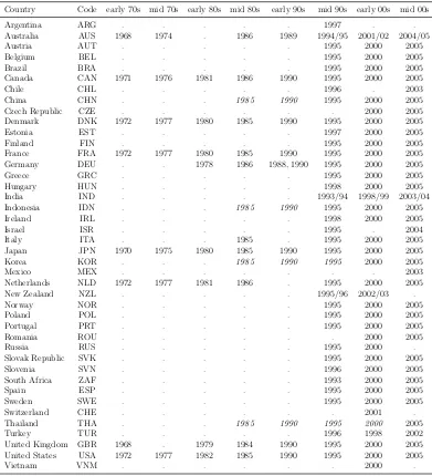
9The countries in our sample (listed in the Online Appendix) account for roughly 80% of world GDP and
We turn to input-output tables for additional information on input use and sector-level
fi-nal expenditure. We take data for benchmark years from the OECD Input-Output Database
and IDE-JETRO Asian Input-Output Tables. Input-output tables are available for all
forty-two countries after 1995, for Asian countries from 1985, and ten major industrialized
coun-tries (the G7 plus Australia, Denmark, and the Netherlands) from the 1970’s.
In combining these data, we face two challenges. First, there are discrepancies across
alternative data sources, both due to differences in definitions and measurement error.
Sec-ond, whereas the national accounts and trade data are annual, the input-output tables are
produced for benchmark years only, which are asynchronous across countries. To resolve
these issues, we prioritize the national accounts data and adjust the commodity trade data
in order to match the levels of aggregate trade in the national accounts. We then use a
con-strained least squares procedure to simultaneously adjust the input-output data to match
the annual production and trade data and extrapolate benchmark data to non-benchmark
years.
The result is a sector-level data set containing gross output (yit), value-added to output
ratios (rit(s)), final demand for domestic and imported goods (fiit and fIit), and domestic
and imported input use matrices (Aiit andAIit) for forty-two countries.10 For goods imports
(s={1,2,3}), we use observed bilateral final and intermediate import shares to splitfIit(s)
andAIit(s, s0) across sources. For the services sector, we apply a proportionality assumption;
we assume that bilateral import shares for final and intermediate services are the same and
equal to the share of each partner in multilateral services imports.
10Because we do not have production or input-output data for countries in the rest of the world, we
2
Changes in Value-Added vs. Gross Exports
Using the framework and data introduced above, we document five stylized time-series facts
regarding changes the ratio of value-added to gross exports over time. We start at the
multilateral level, documenting changes at the world, sector, and country level. We then
examine how proxies for bilateral trade frictions have shaped changes in bilateral
value-added versus gross exports. These serve as focal points in the model accounting analysis
that follows in Section 3.
2.1
World, Sector, and Country Changes
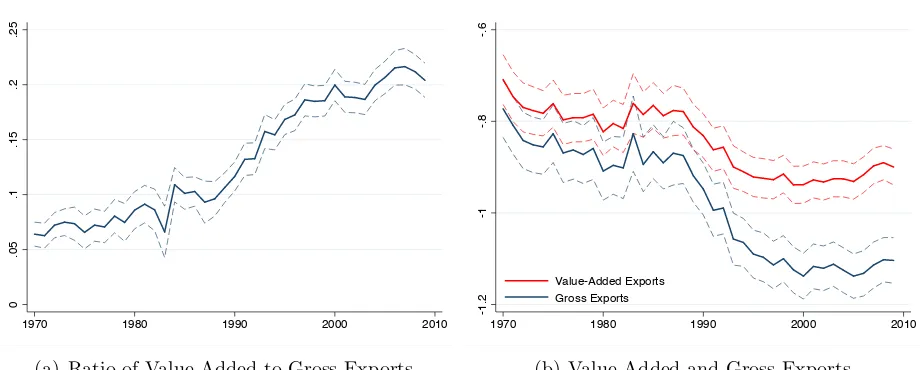
We start at the global level, plotting the ratio of value-added exports to gross exports for
the world as a whole in Figure 1. The ratio of value-added to gross exports declines by
0.08 including the ROW and 0.09 excluding the ROW from 1970-2009. Excluding the 2009
trade collapse, the value-added to export ratio declines by 0.11 including the ROW and by
0.13 excluding the ROW.11This decline is spread unevenly over time. During the 1970-1989
interval, there is only a small net decline value added relative to gross exports, on the order
of a few percentage points. In contrast, value added relative to gross exports fall rapidly, by
8.5 (9.5 excluding the ROW) percentage points from 1990-2008. The decline in the
value-added to export ratio is roughly three times as fast during the 1990-2008 period as during
the pre-1990 period.
To drill down, we disaggregate these global trends along two dimensions, into changes in
value-added to export ratios at the sector level and across countries. We plot sector-level
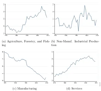
changes in Figure 2. The headline result is that manufacturing is the only sector in which
the value-added to export ratio is falling over time. The ratio is increasing for agriculture
and services and stable in non-manufacturing industrial production.12
11Bems, Johnson and Yi(2010) point to the composition of changes in final expenditure during the 2009
recession to explain why value added rose relative to gross trade. When spending on final goods from sectors with high degrees of vertical specialization (e.g., durable goods) falls, then the ratio of value-added to gross exports rises.
In Figure 3, we plot changes in value-added to export ratios at the country level. Panel
(a) of Figure 3 contains cumulative changes in the ratio of value-added to gross exports
from 1970-2008 at the country level. Nearly all countries experienced declines in the ratio
of value-added to gross exports, but the magnitude of the decline is heterogeneous across
countries. Most experience declines larger than 10 percentage points, though some large
and prominent countries (e.g., Japan, the UK, and Brazil) have smaller declines. Among
countries with large declines, one sees many emerging markets, but also some important
advanced economies (e.g., Germany).
To organize this cross-country variation, we plot the average annual change in the ratio
of value-added to gross exports against the average annual growth rate in real GDP in Panel
(b) of Figure 3. The correlation is negative and statistically significant at the 1% level.
Cumulated over four decades, the point estimate implies that a country at the 90thpercentile
of the growth distribution (5.8% per year) has a decline in the ratio of roughly 0.21 while
a country at the 10th percentile (2.2% per year) has a decline of 0.11. Because emerging
markets on average have higher growth than advanced countries, this also reinforces the
observation above that gross exports have risen more than value-added exports on average
for these countries.
2.2
Bilateral Trade Frictions
Shifting our focus to bilateral country pairs, we describe how changes in bilateral
value-added versus gross exports are shaped by bilateral trade frictions. We focus on two common
proxies for bilateral frictions: distance and regional trade agreements.
The Differential Burden of Distance We are interested in two main questions. First,
how do gross exports (xijt), value-added exports (vaijt), and value-added to export ratios
(V AXijt ≡ vaxijt
ijt ) respond to bilateral distance? Second, how have these responses changed
over time?
To answer these questions, we estimate gravity-style regressions for each of the three
variables of interest:
log(yijt) =φyit+φ y jt +β
y
t log(distij) +εijt, (3)
where yijt ∈ {xijt, vaijt, V AXijt}), {φyit, φ y
jt} are importer-year and exporter-year fixed
ef-fects and βty is the time-varying coefficient on bilateral distance (distij) for outcome y.
For interpretation, it is useful to note that βV AX = βva −βx holds by construction, since
log(V AXijt) = log(vaijt)−log(xijt).
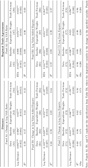
The distance coefficients estimated in Equation (3) are plotted in Figure 4.13 Looking at
the left panel, the ratio of value-added to gross exports is higher for more distant markets.
This is reflected in the separate distance coefficients for gross versus value-added exports
in the right panel. While distance depresses both, gross exports fall more strongly with
distance than do value-added exports – i.e., the absolute value of the distance coefficient
on gross exports is larger than the coefficient on value-added exports in all years. Further,
this differential impact of distance is strengthening over time. The distance coefficient for
the value-added to export ratio has risen from under 0.1 to 0.2. The reason is that distance
coefficient for gross exports has risen (in absolute value) over time, from roughly 0.9 to 1.1.14
13Very small bilateral gross trade flows are often lead to extreme value-added to export ratios, which
distort the point estimates and muddy inference. These outliers are mostly for emerging markets with low quality data during the 1970-1985 period. We remove them by dropping bilateral flows less than one million dollars and value-added to gross export ratios greater than ten.
14In the Online Appendix, we show that changes in these coefficients are robust to adding additional
Regional Trade Agreements We now examine how value-added and gross exports
re-spond to the adoption of regional trade agreements.15
To demonstrate the main result visually, we take an event study approach. We compare
the evolution of the value-added to export ratio for the treatment group of bilateral country
pairs that form new RTA’s during our sample to outcomes for a pair-specific control group
in a window surrounding adoption of the RTA. For country pair (i, j) that forms an RTA,
the control series is the bilateral value-added to export ratio for countries i and j vis-`a-vis
the set of countries with whom both iand j never form an RTA.16
We plot the resulting treatment and control series in Figure 5. Prior to RTA adoption,
value-added to export ratios are quite similar across the treatment and control groups. There
is then a strong divergence between the two, coinciding with adoption of the RTA: for pairs
that adopt an RTA, the value-added to export ratio drops sharply around the adoption date
and then continues to fall for roughly a decade thereafter. This divergence is prima facie
evidence that trade agreements have different effects on gross versus value-added trade.
To formalize these results and control for confounding factors, we turn to panel regressions
of the form:
log(yijt) = φyit+φ y jt+φ
y ij +β
yT radeAgreement
ijt+εyijt, (4)
whereT radeAgreementijt is a collection of indicators for whetheri andj are in a particular
trade agreement at timetandφyij is a country-pair fixed effect.17 We consider several different
specifications for T radeAgreementijt. The first uses a single indicator for whether countries
15We use data on economic integration agreements assembled by Scott Baier and Jeffrey Bergstrand,
covering the 1960-2009 period [September 2015 Revision; http://www.nd.edu/~jbergstr/]. Our RTA indicator takes the value one if a country pair has a free trade agreement or stronger.
16Formally, define T
t(i, j) = vaxijt+vajit
ijt+xjit to be the bilateral value-added to export ratio for (i, j) pairs in
the treatment group. Further, letK(i, j) denote the set of countries with whom bothi and j never form an RTA, and define Ct(i, j) = Pc∈K(i,j)
(vacjt+vajct)+(vacit+vaict)
(xcjt+xjct)+(xcit+xict) to be the value-added to export ratio for
trade betweeniandjwith the control group. Ift= 0 is the year of RTA adoption, then we computeTt(i, j)
andCt(i, j) fort= [−20,20] for each pair and take an unweighted average of each series across all pairs.
17As discussed byBaier and Bergstrand(2007), the pair fixed effect accounts for endogenous adoption of
have an RTA in force, the second distinguishes “shallow” from “deep” agreements, and the
third allows for phase-in effects.18 We estimate this equation using data at five-year intervals
from 1970 to 2009 (the 2005-2009 interval is four years).
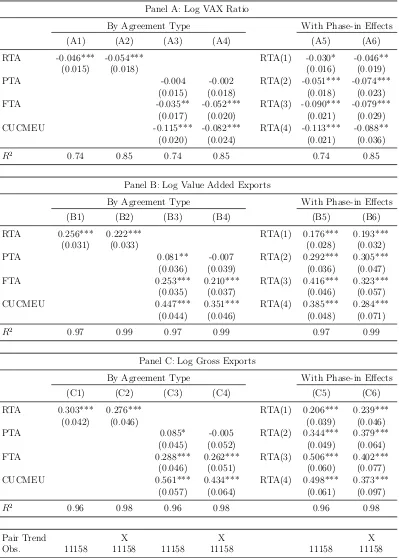
Table 1 reports the estimation results. We find that adoption of trade agreements
low-ers value-added relative to gross exports among countries in those agreements. Using the
simple binary RTA indicator (RT Aijt), the ratio falls by about 5% following adoption of
an agreement. In columns 3 and 4, we split out the effects of different agreements. While
signing a preferential agreement has no impact on the ratio of value-added to gross exports,
adoption of an FTA lowers the ratio of value-added to gross exports. Further, “deeper”
CUCMEU agreements are associated with larger declines than FTAs. Following adoption
of a CUCMEU, the ratio declines between 8-12%, whereas adoption of a FTA is associated
with a drop of 4-5%. The response of gross and value-added trade flows to RTA adoption
are reported in Panels B and C. Consistent with the changes in value-added to export ratios,
we find that gross exports rise more following the adoption of RTAs than do value-added
exports, with larger differences for “deep” agreements.
To quantify adjustment dynamics, we report the coefficients on RTA indicators for specific
periods post-RTA adoption in columns 5 and 6 of Table 1. Consistent with the dynamics in
Figure 5, the impact of RTA adoption appears to grow over time.19 Upon adoption of the
RTA, the ratio of value-added to gross exports falls by 3-5% and then continue to fall over
the duration of the agreement. The total effect levels off at around 9-11%. Value added and
gross exports follow similar adjustment dynamics, with value-added exports rising between
28-39% and gross exports rising between 37-50% in the long run.
18In terms of depth, we distinguish preferential trade agreements (PTA), free trade agreements (FTA),
and customs unions, common markets, and economic unions (CUCMEU). To allow for phase-in effects, we define a set of indicator variables: RT Aijt(1) takes the value 1 in the RTA adoption year,RT Aijt(2) equals
1 in the 5th year,RT Aijt(3) equals 1 in the tenth year, andRT Aijt(4) equals 1 one for years 15 onward.
19Adjustment dynamics may arise for several reasons. First, trade agreements are typically phased in, so
2.3
Summing Up: Five Stylized Facts
To sum up, we have documented five stylized facts. The first is that the ratio of world
value-added to gross exports has fallen over time, by roughly ten percentage points and
mostly post-1990. The second is that the ratio of value-added to gross exports has fallen for
manufacturing, but actually risen outside of manufacturing. The third fact is that changes
have been heterogeneous across countries, with fast growing countries seeing larger declines
in the ratio of their value-added to gross exports. The fourth and fifth facts concern bilateral
changes: declines in value-added to export ratios have been larger for proximate partners
and country pairs that adopted regional trade agreements.
3
What Driving Forces Account for the Facts?
In this section, we ask: what driving forces account for the five stylized facts identified in
Section 2? Are they products of distinct driving forces, or do common driving forces account
for multiple facts simultaneously? These questions are difficult to answer with data alone.
Many features of the global economy have changed over time, and these changes are linked
together: any given candidate driving force (e.g., changes in productivity, endowments, trade
frictions, etc.) leads to changes in multiple aspects of the input-output system. Therefore,
we need a structural equilibrium framework to disentangle competing explanations for the
stylized facts.
We develop an Armington-style model with cross-sector and cross-country input-output
linkages suited to this task. The analysis then proceeds in two steps. First, we use the model
as a measurement device. While we are able to collect data on some driving forces (e.g.,
changes in factor inputs and productivity across countries), it is difficult to directly measure
others. Specifically, trade costs are difficult to measure in a comprehensive, consistent way
through time [Anderson and van Wincoop (2004)]. Changes in preferences and production
Therefore, we combine the model and data to infer them.20
Second, we apply the model in a series of counterfactuals to assign responsibility to
particular driving forces for changes in value-added to gross exports in the data. To preview
the main result, we demonstrate that changes in trade frictions provide a unifying explanation
for all five stylized facts. Following up on this result, we use the model to study the role of
particular components of trade frictions in greater detail in Section 4.
3.1
Framework
This section lays out the core elements of the model. Details regarding the model and its
solution are collected in the Online Appendix.
3.1.1 Economic Environment
Each country combines domestic factors with purchased intermediate inputs to produce a
unique, Armington differentiated good in each sector. Denoting the quantity of the good
produced by country i in sector s asQit(s), the production function takes the form:
Qit(s) =
λVi (s)1−σVit(s)σ+ (1−λVi (s))
1−σX
it(s)
1/σ
, (5)
Vit(s) =Zit(s)Kit(s)αLit(s)1−α, (6)
Xit(s) =
"
X
s0
λXit(s0, s)1−σXit(s0, s)σ
#1/σ
, (7)
Xit(s0, s) =
" X
j
Xjit(s0, s)κ
#1/κ
, (8)
20Our approach to measuring trade frictions is closely related to “ratio-type estimation” in gravity models
where the λ’s denote CES share parameters.21 In words, gross output is produced by
com-bining real value added Vit(s) and a composite intermediate inputXit(s). Real value added
is a Cobb-Douglas composite of capitalKit(s) and laborLit(s), combined with productivity
Zit(s). The composite input is formed by combining composite inputs purchased from
dif-ferent sectors, where Xit(s0, s) is the quantity of a composite input from sector s0 purchased
by sectorsin country i. Xit(s0, s) is itself a composite of inputs sourced from different
coun-tries, whereXjit(s0, s) is the quantity of inputs from countryj embodied inXit(s0, s). Gross
output is used as both a final and intermediate good. We assume that there are iceberg
frictions associated with purchasing inputs and final goods. These frictions apply to both
domestic and imported goods, and they differ by sectors (or sector-pairs) and end use. The
market clearing condition for gross output is:
Qit(s) =
X
s0 X
j
τijtX(s, s0)Xijt(s, s0) +
X
j
τijtF(s)Fijt(s), (9)
where the indexing on trade costs (the τ’s) is the same as for goods flows.
A composite final good in each country is produced by aggregating final goods purchases:
Fit =
" X
s
λFit(s)1−ρFit(s)ρ
#1/ρ
with Fit(s) =
" X
j
Fjit(s)κ
#1/κ
, (10)
where Fit(s) is the quantity of a sector-level composite goods and Fjit(s) is the quantity of
final goods from sector s purchased by country ifrom country j.
This composite final good is used for both consumption (Cit) and investment (Iit), with
Fit =Cit+Iit. As is standard, investment determines the aggregate capital stock: Ki,t+1 =
Iit+ (1−δit)Kit, where Iit is real investment and δit is the depreciation rate. We assume
21We impose constant share parametersλV
i (s) in Equation (5) because we do not have the gross output
price data necessary to infer changes inλV
i (s). Because we omit CES weight parameters in Equation (8) and
that each country is endowed with labor Lit, which is inelastically supplied to firms. The
market clearing conditions for capital and labor are: Kit=PsKit(s) and Lit =PsLit(s).
To close the model, we assume that real investment is proportional to final expenditure,
as inLevchenko and Zhang(2016). That is,Iit=sitFit, wheresitis an exogenous investment
share parameter.22 Together with the representative consumer’s budget constraint, this pins
down consumption. The budget constraint takes the formpFitFit =
P
s[ritKit(s)+witLit(s)]+
Tit, where pFit is the price of the final composite, rit and wit are the prices of capital and
labor, and Tit is a nominal transfer received by agents in countryi. We assume Tit (i.e., the
trade balance) is exogenous.
Following Dekle, Eaton and Kortum (2008), we solve for the model’s competitive
equi-librium in changes. In doing so, we take changes in trade balances, productivity, labor
endowments, and the investment share as given. We define the equilibrium and collect the
equilibrium conditions (in levels and changes) in the Online Appendix.
3.1.2 Quantification
To operationalize the model, we need to assign values to model parameters and collect data on
exogenous forcing variables. Further, we need to back changes in unknown parameters (e.g.,
trade frictions, preference/technology parameters) out of the data. We provide an overview
of the procedure here, with details in the Online Appendix. As a practical matter, we use a
two-sector version of the model and data to simplify the parametrization, computation, and
counterfactual analysis. The two sectors are manufacturing (m) and non-manufacturing (n)
sectors (s∈ {m, n}).
Parameters and Exogenous Variables The parameter κ governs substitution across
countries in final and intermediate input purchases. We set κ = 0.75 – corresponding to
22We discuss this assumption further in the Online Appendix. We back changes in s
it out of data and
an elasticity of substitution of 4 – to match standard estimates of the trade elasticity.23
The parameter ρ governs the cross-sector elasticity of substitution in final demand, while
σ governs substitution between real value added and inputs, as well as across inputs from
different sectors. We set σ = ρ = −1, corresponding to an elasticity of substitution equal
to 0.5. This means that manufacturing and non-manufacturing sectors are complements in
final demand, and that value added and inputs, and inputs across sectors, are complements
on the production side. These assumptions are both supported by existing evidence.24
We also need values for the parameters {α, δit} and the exogenous forcing variables
{sˆit,Tˆit,Zˆit(s),Lˆit}. We set α = 0.3, and we set the remaining values based on our
input-output data and the Penn World Tables.
Trade Frictions and Expenditure Weights We introduce the following notation and
nomenclature to clarify what aspects of trade frictions and preference/technology
parame-ters we are able to back out of the data.25 First, we normalize international iceberg frictions
relative to domestic frictions: ωXjit(s0, s) ≡ τjitX(s0, s)/τiitX(s0, s) and ωjitF (s) ≡ τjitF (s)/τiitF(s).
Henceforth, we refer to ωjitX(s0, s) and ωjitF (s) as “trade frictions,” since they govern
sub-stitution across country sources. Given this normalization of the international frictions,
we define a second set of “expenditure weights” that combine CES weight parameters and
domestic frictions: ωX
it(s
0, s) ≡ λX it(s
0, s)(σ−1)/στX iit(s
0, s), ωF
it(s) ≡ λFit(s)(ρ
−1)/ρτF
iit(s). These
expenditure weights govern substitution across sectors in sourcing inputs and final goods.
To compute changes in trade frictions and expenditure weights, we need additional price
23This is the mean SITC 3-digit trade elasticity reported in Broda and Weinstein (2006). Note that we
implicitly restrictκto be the same in both sectors. This is consistent with the fact that the mean Broda-Weinstein elasticity estimates for non-manufacturing (SITC 1-4) and manufacturing (SITC 5-8) are both close to 4.
24The low final expenditure elasticity is consistent with the fact that both the share of non-manufacturing
in final expenditure and the relative price of non-manufacturing output have been rising over time. This observation motivates low elasticities in the structural change literature [Ngai and Pissarides(2007), Herren-dorf, Rogerson and Valentinyi(2013)]. Low substitutability in production is consistent with recent estimates byAtalay(2015) andOberfield and Raval(2015).
25If domestic trade frictions are constant, then we could identify changes in the level of international trade
data, not already included in our global input-output data. We need changes in the price
of real value added in each sector ˆpV
i (s), and changes in the price of final expenditure ˆpFi .
Drawing on national accounts sources, we set ˆpV
i (s) equal to changes in GDP deflators in
the manufacturing and non-manufacturing sectors, and we set ˆpF
i equal to changes in the
ratio of nominal to real final expenditure.26 We use this price data, along with first order
conditions and price indexes from the model, to solve for changes in the trade frictions and
expenditure weights implied by changes in expenditure shares over time.
The estimates we recover via this procedure are sensible and consistent with related
work.27 Globally, iceberg trade frictions decline by 35% from 1970-2009. There is significant
dispersion in the magnitude of the declines across countries, and declines are strongly
corre-lated with changes in openness (as expected). Trade frictions decline both in manufacturing
and non-manufacturing sectors, though declines are somewhat larger for manufactures. As
we discuss further in Section 4.2, RTA adoption predicts declines in trade frictions at the
bilateral level. As for the expenditure weights, changes in final goods expenditure weights
are similar across manufacturing and non-manufacturing sectors, while input expenditure
weights have tended to pull input expenditure toward non-manufacturing.
3.2
Counterfactuals
We now conduct counterfactuals in the model to assess the role of trade frictions in
ex-plaining changes in value-added to export ratios. The first counterfactual holds both trade
frictions and expenditure weights constant at their 1970 levels. Following our notation above,
ˆ
ωX it(s
0, s) = ˆωF
it(s) = ˆωjitX(s
0, s) = ˆωF
jit(s) = 1, and the exogenous variables{sˆit,Tˆit,Zˆit(s),Lˆit}
evolve as in the data. We treat this simulation as the baseline against which we assess the
relative importance of trade versus expenditure weights.
26We take price changes and exchange rates (to convert GDP and final expenditure deflators to a common
currency) from the UN National Accounts Database, with one exception. For China, we take ˆpV
i (s) from
the World Development Indicators, since it is missing for many years in the UN Database.
27For example, our estimated changes in trade frictions are comparable to estimates by Jacks, Meissner
The second and third counterfactuals decompose the gap between this baseline and the
data into components due to trade frictions versus expenditure weights. The second
coun-terfactual holds expenditure weights constant at their 1970 levels (ˆωX
it(s
0, s) = ˆωF
it(s) = 1)
and allows trade frictions to evolve as implied by the data. The third counterfactual holds
trade frictions constant at their 1970 levels (ˆωX
jit(s
0, s) = ˆωF
jit(s) = 1) and allows expenditure
weights to evolve as implied by the data.
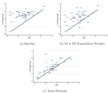
Figure 6 plots changes in value-added to export ratios for the world as a whole.28 In
the baseline simulation of the model, there is virtually no long run change in the ratio of
value-added to gross exports. This means that changes in country size and sectoral output
composition, driven by both productivity and factor endowments in the baseline simulation,
do not explain the decline in the ratio of value-added to gross exports. Interestingly, these
results obtain even though world trade does rise substantially in this counterfactual
simu-lation: the baseline model alone accounts for about 40% of the growth of trade since 1970.
The stability of the value-added to export ratio simply means that this gross trade growth
is matched by increases in value-added exports. Adding expenditure weights to the model
does little to change this result. In contrast, allowing trade frictions to change generates a
simulated series that captures the evolution of the ratio of value-added to gross exports well.
Figure 7 plots changes in value-added to export ratios at the sector level. Here again,
the baseline simulation performs poorly. It accounts for only a small part of the declining
value-added to export ratio in manufacturing, and the ratio in non-manufacturing moves
in the wrong direction entirely. Expenditure weights close the gap between simulation and
data, but their explanatory power is limited. Where they play a role is in explaining the
medium-term dynamics of the manufacturing VAX ratio, capturing the pre-1990 slowdown
and post-1990 acceleration in the rate of decline. Trade frictions are important in explaining
changes in the VAX ratio for both sectors. They explain changes in the non-manufacturing
sector almost completely, and explain more than half of the steady decline in manufacturing.
28To match the simulation, the ‘true’ value-added to export ratios in these figures are computed using a
Figure 8 plots changes in value-added to export ratios from 1975-2005 at the country
level. As in previous figures, both the baseline simulation and the simulation with changes
in expenditure weights struggle to match the data. The baseline simulation under-predicts
the magnitude of the declines, particularly for countries with large declines. Expenditure
weights generate additional dispersion, but do little to improve the overall fit. Again, changes
in trade frictions bring the simulated data in line with actual changes for most countries.
The visual impression conferred by the figures is confirmed by more systematic measures of
the goodness of fit. The correlations between simulations and data are 0.39 in panels (a)
and (b), and 0.69 in panel (c). Mean errors are 0.11, 0.08, and 0.03 for the three simulations
(in order).
Turning to bilateral flows, we estimate the same regressions used to describe the stylized
facts in Section 2 using simulated data. The left panel of Table 2 includes long difference
regressions that focus on the role distance, while the right panel examines the role of RTAs.
Consistent with the discussion above, the baseline simulation fails badly at explaining the
distance or RTA results. Input-output and final goods expenditure weights do a little better
for the distance effects. However, it looks initially like they help explain declines in the
value-added to export ratio surrounding RTAs. This apparent good performance is misleading.
Looking at Panels B and C, changes in input-output and final goods expenditure weights
lower the simulated bilateral VAX ratio because they lead bilateral value-added exports to
fall post-RTA adoption, while gross exports are unchanged – both these results are grossly
inconsistent with the data. Changes in trade frictions, instead, do well in matching both the
distance and RTA evidence. They predict both the decline in the VAX ratio and the rise in
value-added and gross exports post-RTA adoption.
To sum up, we set out to evaluate the role of trade frictions in explaining the data. The
counterfactuals point to changes in trade frictions as the most important force underlying all
five stylized facts. We therefore shift our attention to examining the role of trade frictions
4
Interpreting the Role of Trade Frictions
To interpret the role of trade frictions in explaining the five facts, we unpack the
fric-tions themselves. First, we distinguish trade fricfric-tions by sector (manufacturing vs.
non-manufacturing) and end use (final vs. intermediate goods). We simulate the model with
each set of frictions independently, and we use these simulations together with accounting
relationships to examine the mechanics underlying changes in multilateral value-added to
export ratios. Second, we hone in on bilateral frictions to examine the role of policy changes
– specifically, RTA adoption – in driving changes in value-added to export ratios.
4.1
Unpacking Trade Frictions
We run four new counterfactual simulations with changes in (1) final non-manufacturing
trade frictions, holding other trade frictions fixed (ˆωF
jit(m) = ˆωjitX(s
0, s) = 1), (2) input
non-manufacturing trade frictions (with ˆωF
jit(s) = ˆωXjit(m, s) = 1), (3) final manufacturing trade
frictions (with ˆωF
jit(n) = ˆωjitX(s0, s) = 1), and (4) input manufacturing trade frictions (with
ˆ
ωjitF (s) = ˆωXjit(n, s) = 1). In all these simulations, expenditure weights are held constant
at 1970 levels (ˆωitX(s0, s) = ˆωitF(s)). These four simulations decompose the Trade Frictions
simulation presented previously, so we compare them that simulation in the analysis below.
4.1.1 Results
Along all three dimensions of the multilateral data – for the world, countries, and
sec-tors – trade frictions for manufactures are more important than trade frictions for
non-manufacturing output. Further, among non-manufacturing trade frictions, frictions for inputs
are more important than frictions for final goods.
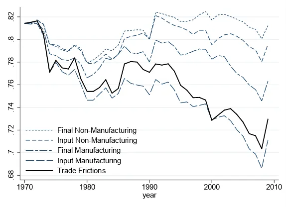
In Figure 9, we plot the four simulations for the world. As is evident, changes in trade
frictions for manufacturing goods used as inputs generate a large decline in the simulated
the ratio also declines due to changes in frictions for final manufacturing goods (particularly
post-1990).
Turning to sectors, we plot value-added to export ratios in the four simulations in Figure
10. Here again, manufacturing trade frictions do the bulk of the work. Frictions on
manu-factured inputs are most important in accounting for the decline in the manufacturing ratio,
though frictions on final manufactures matter as well. For the non-manufacturing sector,
final manufacturing frictions are most important, with input-manufacturing frictions also
playing a role in explaining the rising value-added to export ratio in this sector.
At the country level, all four simulations generate data that is positively correlated with
the composite Trade Frictions simulation, and roughly equally so (the correlations are all near
0.5). However, simulations with changes in non-manufacturing frictions alone underpredict
the size of the declines in value-added to export ratios: the mean error is 0.10 in simulation
(1) and 0.08 in simulation (2). In contrast, simulations with changes in manufacturing
frictions generate significant declines in value-added to export ratios, with a mean error of
0.04 in simulation (3) and -0.006 in simulation (4). From this, we conclude that frictions for
manufactured inputs are most important in explaining country-level ratios as well.
4.1.2 Interpretation
To interpret these results, we combine accounting results with the intuitive mechanics of
the model. We start by explaining the link between sector-level trends and the world-level
results, and then we discuss sector trends themselves in detail. We conclude with a brief
discussion of heterogeneity across countries.
Aggregating Sector Trends The world value-added to export ratio can be written as a
trade-weighted average of sector-level ratios: V AXt =
P
s
Xt(s)
Xt
V AXit(s). This suggests
into components due to changes inV AXt(s) versus sectoral trade shares:
∆V AXt=
X
s
¯
ωt(s)∆V AXt(s)
| {z }
Within
+X
s
V AXt(s)∆ωt(s)
| {z }
Between
, (11)
where ∆ denotes time differences, ¯ωt(s)≡ 12(ωt(s) +ωt−1(s)) with ωt(s) =
P
i6=jxijt(s) P
i6=j P
sxijt(s), and
V AXt(s)≡ 12(V AXt(s) +V AXt−1(s)).
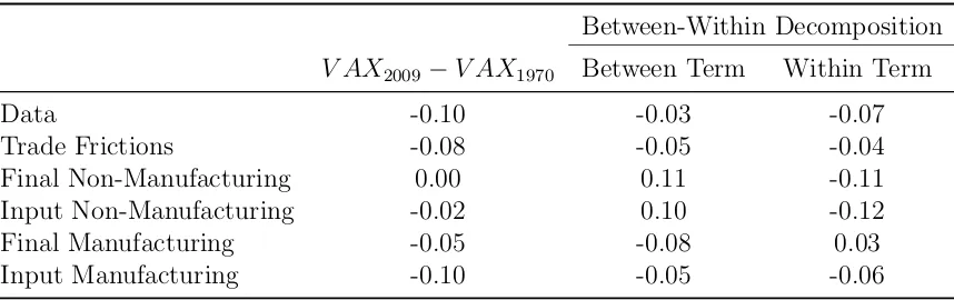
We report this decomposition in actual and simulated data in Table 3. In the data, both
the between and within terms are negative, and the within term is larger than the between
term. The within term is obviously driven by the decline in the manufacturing value-added to
export ratio, which dominates the rise in the non-manufacturing ratio because manufactures
account for 60-70% of world trade. The between term is negative because the share of
manufacturing rises over the period, and the level of the value-added to export ratio is lower
in manufacturing than non-manufacturing. The between term is modest in size because
changes in trade shares are small (a few percentage points).
Turning to simulation results, the Trade Frictions counterfactual generates negative
within and between effects, consistent with the data. Breaking the trade frictions apart,
only the simulation with declines in trade frictions for manufactures used as inputs matches
this pattern (and hence the data). All the other trade frictions simulations generate results
that point in the wrong direction for explaining the data, in one way or another.29 Falling
input frictions for manufacturing goods lower the value-added to export ratio in
manufac-turing (as in Figure 10), and this drives the within effect. They also increase the share of
manufactures in trade, which accounts for the negative between effect.
29Non-manufacturing trade costs generate negative within effects, but (counterfactual) positive between
Sector Trends We now turn our attention to explaining the sector trends themselves.
To do this, it is helpful to appeal to the tight (empirical and conceptual) link between
value-added to export ratios and the domestic content of exports. Domestic content is
the value of exports less the import content of exports, and it measures the amount of
domestic value added needed to produce exports [Hummels, Ishii and Yi (2001)]. As an
empirical matter, sector-level domestic content is approximately equal to sector-level
value-added exports [Johnson and Noguera (2012a)]. We therefore use domestic content as a
proxy for value-added exports in interpreting sector trends, because domestic content is a
mathematically simpler object to interpret.
Formally, domestic content can be written as DCit = Rit(I −ADit)−1Xit, where Rit
is a matrix with sector-level value-added to output ratios rit(s) along the diagonal, ADit
is the domestic input-output matrix, and Xit is the export vector of country i.30 The
domestic content to gross export ratio at the sector level is then: DCit(s)/Xit(s) =wit(s, s)+
wit(s, s0)(Xit(s0)/Xit(s)), where the weightswit(s, s0) are the elements ofRit(I−ADit)−1 and
indicate how much domestic content from sector s is needed to produce exports from sector
sector s0. These weights depend both on cross-sector input linkages – how much output
from sector s is used in producing exports in sector s0 (via (I−ADit)−1) and the
imported-input intensity of production in sector s (via Rit). Finally, note that this ratio depends
directly on export composition, because domestic content is both exported directly via a
sector’s own exports and indirectly via exports of other sectors. As indirect exports rise,
then DCit(s)/Xit(s) will rise.
Putting these observations to work, falling frictions on manufactured inputs increase
foreign sourcing in the manufacturing sector, and hence drive down DCit(m)/Xit(m) in
manufacturing. They also simultaneously drive up DCit(n)/Xit(n), because they raise the
share of manufactures in trade, which in turn raises the level of indirect exports by the
non-manufacturing sector. Falling frictions on final manufactures have similar
composi-30To interpret this, (I−A
Dit)−1Xit is the amount of domestic gross output needed to produce exports,
tional effects, which explains why they too raise the value-added to export ratio in
non-manufacturing. These compositional effects also contribute to the decline in the value-added
to export ratio in manufacturing, since they lower indirect exports of manufacturing value
added, by reducing (Xit(n)/Xit(m)). Together these mechanisms explain the dominant role
of manufacturing trade frictions in explaining the trends in sector-level VAX ratios, depicted
in Figure 9.
Country-Level Changes Looking at cross-country changes in value-added to export
ra-tios, the same basic within and between forces come into play as in the aggregate. As at
the world level, the value-added to export ratio in manufacturing declines in virtually all
countries. The large majority of countries also see increases in value-added to export ratios
in non-manufacturing. Further, the level of the non-manufacturing ratio is higher than the
manufacturing VAX essentially everywhere.
The main difference is that between effects are more important in explaining
country-level changes than they are at the world country-level. The reason is that changes in trade shares
are substantially larger at the country-level than in the aggregate, so they play a larger role
in the between-within decomposition. Countries with the largest declines in value-added to
export ratios tend to have very large, negative between effects (i.e., tend to see large increases
in the share of manufacturing exports). Because declines in manufacturing trade frictions
increase manufacturing exports, they are important in explaining cross-country variation as
well.
4.2
The Role of Regional Trade Agreements
We now turn to assessing the role of regional trade agreements in our results. Our first
goal is to confirm that Fact 5 – that RTAs lower bilateral value-added to export ratios –
is explained entirely by changes in bilateral trade costs surrounding RTA adoption. Our
is explained by the spread of RTAs over time.
The approach we take is to simulate a counterfactual world in which no new regional trade
agreements were adopted between 1970 and 2009, and then we compare this to data. To
do this, we need to construct counterfactual trade frictions that capture how trade frictions
would have evolved in the absence of post-1970 RTAs. We proceed in two steps (see the
Online Appendix for details). In the first step, we model trade frictions as a function of
RTAs and other unobserved time-varying importer, exporter, and pair-specific factors. We
then estimate the impact of RTA adoption by regressing changes in measured frictions (for
each input sector-pair or final goods sector separately) on fixed effects and trade agreement
indicators. In the second step, we use the estimated RTA coefficients to adjust the measured
trade frictions, removing changes in trade frictions due to RTA adoption.31
As expected, our estimates indicate that RTA adoption lowers bilateral trade frictions
among adopting countries.32 To summarize the magnitudes, trade frictions fall by roughly
7-8% after RTA adoption when we measure RTA adoption using a simple binary indicator.
When we allow for dynamic phase-in effects, RTAs lower trade frictions by 16-20% in the
long run. We view these estimates as lower and upper bounds on plausible RTA-impacts.
When we separate agreements, we find an ordering of changes in trade frictions consistent
with our previous gravity results: deep trade agreements are associated with larger declines
in trade frictions than shallower agreements.
Using these results, we simulate the model with counterfactual trade frictions, removing
post-1970 RTAs and allowing all other driving forces (including changes in expenditure
weights) to evolve as implied by data. This means that deviations between simulated and
true data in this set of results reflect only the removal of RTAs. To frame the analysis,
recall that we showed (in Table 2) that changes in trade frictions can account for declines in
value-added relative to gross exports following adoption of regional trade agreements (Fact
31For pairs that form a new RTA after 1970, trade frictions equal measured values prior to RTA adoption
and then are adjusted upward post-RTA as if the RTA were never signed. For all pairs that either never form an RTA or already had an RTA in force in 1970, trade frictions evolve as in the data.
5). We now demonstrate that changes in bilateral frictions attributable to RTA adoption
drive this result.
Using the simulated data, we re-estimate the baseline regressions specifications used
previously to document RTA effects. Because we have removed changes in trade frictions
attributable to RTAs, we expect RTAs to have no effect on bilateral value-added to export
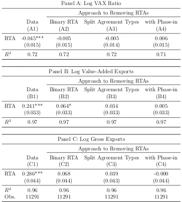
ratios in these regressions. In fact, that is exactly what we find. In Panel A of Table 4, the
RTA-coefficient is numerically close to, and statistically indistinguishable from, zero. This
holds regardless of the technique we use to remove RTAs. Further, this result reflects zero
impact of regional agreements on both value-added exports (Panel B) and gross exports
(Panel C) when RTAs are removed. These results imply that RTA-induced changes in
bilateral trade frictions alone drive the differential response of bilateral value-added versus
gross trade that we observe in the data post-RTA adoption.
An important remaining question is: does the spread of RTAs also help explain the global
decline in the ratio of value-added to gross exports? The answer is that post-1970 RTAs can
explain roughly 6-15% of the overall decline. With RTA effects estimated using a binary
RTA indicator, the ratio of value-added to gross exports for the world as a whole falls by
about 6% less in the counterfactual than in the data. When we split agreements by type,
the ratio of value-added to gross exports falls by about 13% less in the counterfactual than
in the data. Allowing for phase-in effects, the ratio falls by about 15% less than in the data.
These magnitudes are sizable given that only about a third of all country pairs adopt RTAs
during the sample period, and many of these post-1990 agreements have yet to reach their
peak impact. We conclude that the spread of RTAs has played a significant quantitative role
5
Conclusion
With the rise of cross-border supply chains, conventional (gross) trade data is an increasingly
misleading guide to how value added is traded in the global economy. In this paper, we
characterized changes in gross versus value-added trade over four decades. Value-added
exports are falling relative to gross exports, implying double counting in gross trade data is
more pervasive today than in the past. Importantly, gaps between gross and value-added
exports are unevenly distributed across time, sectors, countries, and bilateral partners. These
differences imply that shifting from a gross to value-added view of trade changes the relative
openness of sectors or countries, and the relative importance of bilateral trade partners for
a given country.
Using a structural gravity model, we found that changes in trade frictions play a
first-order role in explaining not only global trends, but also differences across countries, sectors,
and bilateral partners. We emphasize in particular that regional trade agreements have led to
declines in value-added relative to gross trade among adopting partners, such that the spread
of RTAs over time can account for 15% of the decline in the world value-added to export
ratio over time. In contrast, other major structural changes in the global economy (e.g.,
the increasing weight of emerging markets in global GDP) play a minimal role. Changes in
sector-level patterns of input use and demand are also relatively unimportant, as compared
to the role of trade frictions.
Our results have a number of implications for future research. First, the value-added
data we provide are immediately useful for parameterizing quantitative models. Because
the value-added content is falling over time, shifting from gross to value-added export data
in empirical applications is more important now than ever. Second, the large role of trade
frictions in explaining changes in gross versus value-added trade calls for re-visiting classic
questions about the burden of trade frictions. For example, how do gross trade frictions map
into reduced form frictions for trading value added, or how do RTAs induce trade creation
in producing value added, one can immediately convert value-added exports into bilateral
measures of factor/task trade. Therefore, the type of value-added data we provide should
be useful in analyzing models of factor/task trade, including the role of factor/task trade in
References
Anderson, James E., and Eric van Wincoop.2004. “Trade Costs.”Journal of Economic
Literature, 42(3): 691–751.
Antr`as, Pol.2016.Global Production: A Contracting Perspective. Princeton, NJ:Princeton
University Press.
Atalay, Enghin. 2015. “How Important are Sectoral Shocks?” Unpublished Manuscript,
University of Wisconsin.
Baier, Scott L., and Jeffrey H. Bergstrand.2007. “Do Free Trade Agreements Actually
Increase Members’ International Trade?” Journal of International Economics, 71: 72–95.
Bems, Rudolfs, Robert C. Johnson, and Kei-Mu Yi. 2010. “Demand Spillovers and
the Collapse of Trade in the Global Recession.” IMF Economic Review, 58(2): 295–326.
Broda, Christian, and David Weinstein. 2006. “Globalization and the Gains from
Variety.”The Quarterly Journal of Economics, 121(2): 541–585.
Caliendo, Lorenzo, and Fernando Parro. 2015. “Estimates of the Trade and Welfare
Effects of NAFTA.” The Review of Economic Studies, 82(1): 1–44.
Daudin, Guillaume, Christine Rifflart, and Daniele Schweisguth.2011. “Who
Pro-duces for Whom in the World Economy?” Canadian Journal of Economics, 44: 1403–1437.
Dekle, Robert, Jonathan Eaton, and Samuel Kortum. 2008. “Global Rebalancing
with Gravity: Measuring the Burden of Adjustment.” IMF Staff Papers, 55(3): 511–540.
Eaton, Jonathan, Samuel Kortum, Brent Neiman, and John Romalis.forthcoming.
“Trade and the Global Recession.” American Economic Review.
Feenstra, Robert C. 1998. “Integration of Trade and Disintegration of Production in the
Global Economy.” Journal of Economic Perspectives, 12(4): 31–50.
Feenstra, Robert C., and Gordon H. Hanson. 1999. “The Impact of Outsourcing and
High-Technology Capital on Wages: Estimates for the United States, 1979-1990.” The
Quarterly Journal of Economics, 114(3): 907–940.
Freund, Caroline, and Emmanuel Ornelas. 2010. “Regional Trade Agreements.”
An-nual Review of Economics, 2: 139–166.
Grossman, Gene M., and Esteban Rossi-Hansberg. 2008. “Trading Tasks: A Simple
Theory of Offshoring.” American Economic Review, 98(5): 1978–1997.
Head, Keith, and Thierry Mayer. 2014. “Gravity Equations: Workhorse, Toolkit, and
Cookbook.” InHandbook of International Economics. Vol. 4, , ed. Gita Gopinath, Elhanan