Simulation of rear surface contamination for a simple bluff body

warwick.ac.uk/lib-publications

Original citation:

Gaylard, A. P., Kabanovs, A., Jilesen, J., Kirwan, Kerry and Lockerby, Duncan A.. (2017)

Simulation of rear surface contamination for a simple bluff body. Journal of Wind

Engineering and Industrial Aerodynamics, 165. pp. 13-22.

Permanent WRAP URL:

http://wrap.warwick.ac.uk/86817

Copyright and reuse:

The Warwick Research Archive Portal (WRAP) makes this work of researchers of the

University of Warwick available open access under the following conditions.

This article is made available under the Creative Commons Attribution 4.0 International

license (CC BY 4.0) and may be reused according to the conditions of the license. For more

details see:

http://creativecommons.org/licenses/by/4.0/

A note on versions:

The version presented in WRAP is the published version, or, version of record, and may be

cited as it appears here.

Contents lists available atScienceDirect

Journal of Wind Engineering

and Industrial Aerodynamics

journal homepage:www.elsevier.com/locate/jweia

Simulation of rear surface contamination for a simple blu

ff

body

A.P. Gaylard

, A. Kabanovs

, J. Jilesen

, K. Kirwan

, D.A. Lockerby

a_{Jaguar Land Rover, Banbury Road, Gaydon, Warwick CV35 ORR, UK}

b_{WMG, International Manufacturing Centre, University of Warwick, Coventry CV4 7AL, UK} c_{Aeronautical and Automotive Engineering, Loughborough University, Leicestershire LE11 3TU, UK} d_{Exa Corporation, 55 Network Dr, Burlington, MA 01803, USA}

e_{WMG, International Manufacturing Centre, University of Warwick, Coventry CV4 7AL, UK} f_{School of Engineering, University of Warwick, Coventry CV4 7AL, UK}

A R T I C L E I N F O

Keywords:

CFD VLES Aerodynamics Surface contamination Windsor body Lattice Boltzmann

A B S T R A C T

Predicting the accumulation of material on the rear surfaces of square-backed cars is important to vehicle manufacturers, as this progressively compromises rear vision, vehicle visibility and aesthetics. It also reduces the effectiveness of rear mounted cameras. Here, this problem is represented by a simple bluffbody with a single sprayer mounted centrally under its rear trailing edge.

A Very Large Eddy Simulation (VLES) solver is used to simulate both the aerodynamics of the body and deposition of contaminant. Aerodynamic drag and lift coefficients were predicted to within +1.3% and−4.2% of their experimental values, respectively. Wake topology was also correctly captured, resulting in a credible prediction of the rear surface deposition pattern.

Contaminant deposition is mainly driven by the lower part of the wake ring vortex, which advects material back onto the rear surface. This leads to a maximum below the rear stagnation point and an association with regions of higher base pressure.

The accumulation of mass is linear with time; the relative distribution changing little as the simulation progresses, implying that shorter simulations can be compared to longer experiments. Further, the rate of accumulation quickly reaches a settled mean value, suggesting utility as a metric for assessing different vehicles.

1. Introduction

The following presents a numerical simulation of rear surface contamination for a simple bluffbody, representing a road vehicle. It explores the interaction of an idealised tyre spray with a vehicle base wake and the resulting accumulation of material on the rear surface.

This models a significant issue: the accumulation of contaminants (soil, tyre debris, etc.) on the rear surfaces of cars diminishes both drivers’vision and vehicle visibility as material is deposited on lights and the rear screen. In addition, the aesthetic appeal of the vehicle may be reduced and soil transferred to users’hands and clothes as they access the rear load space via the tailgate. These processes have the potential to undermine customers’ perceptions of product quality (Gaylard et al., 2014).

The main contaminant source for these surfaces is the spray generated by the vehicle's own rear tyres, as they move over wet road (Jilesen et al., 2013). This is advected into the base wake and subsequently deposited onto the vehicle's rear surfaces. The coupling

with wakeflows, and hence vehicle aerodynamic performance, means that this issue must be addressed concurrently with aerodynamic drag during the development process.

It has long been appreciated that square-backed vehicles such as hatchbacks, estates, and SUVs are particularly susceptible to this issue (Maycock, 1966) along with bus bodies (Lajos et al., 1986). Therefore this work uses a square-backed bluffbody to represent vulnerable car designs.

Simplified bodies, which represent a few salient geometric features, are widely used in automotive aerodynamics, for an overview of this practise seeLe Good and Garry (2004). They enable key processes to be investigated without the myriad interactions seen in production vehicles, or having to cope with their geometric complexity. In essence, they provide an improved signal-to-noise ratio, by omitting geometry responsible for generatingflow features not significant for the class of problem under investigation.

However, this potentially useful approach has yet to be widely applied to the rear surface contamination problem. In one of the few

http://dx.doi.org/10.1016/j.jweia.2017.02.019

Received 27 January 2016; Received in revised form 10 February 2017; Accepted 15 February 2017 ⁎_{Corresponding author at: Jaguar Land Rover, Banbury Road, Gaydon, Warwick CV35 ORR, UK.}

E-mail addresses:[email protected],[email protected](A.P. Gaylard),[email protected](A. Kabanovs),[email protected](J. Jilesen),

[email protected](K. Kirwan),[email protected](D.A. Lockerby).

Journal of Wind Engineering & Industrial Aerodynamics 165 (2017) 13–22

0167-6105/ © 2017 The Authors. Published by Elsevier Ltd. This is an open access article under the CC BY license (http://creativecommons.org/licenses/BY/4.0/).

examples published,Hu et al. (2015)demonstrate the use of amodified version of the MIRA Reference Model in computationalfluid dynamics (CFD) simulations of the problem, but provide no comparative experi-mental data for either the aerodynamics of the model or deposition of the contaminant.

In contrast, the CFD investigation ofKabanovs et al. (2016)used a well-known simple bluffbody and provided some contaminant deposi-tion patterns obtained from wind tunnel experiments. However, their computational work did not account for realistic wake unsteadiness.

Hence, this work extends that ofKabanovs et al. (2016), applying an unsteady eddy-resolving CFD simulation to their simple test case. Doing so provides additional insights into spray advection into the wake, its distribution through the wake and the subsequent pattern of deposition. The latter permits some limited qualitative comparison of the numerical simulation against their experimental data. Data from the literature are also used to assess the degree to which the CFD simulation captures the aerodynamics behaviour of the bluffbody, in terms of drag and lift force prediction along with wake topology.

In addition, guidance is provided on the numerical simulation of this issue; specifically coping with the mismatch between the sampling times available in experiments with those economically obtainable with unsteady CFD simulation.

2. Approach

2.1. Bluffbody

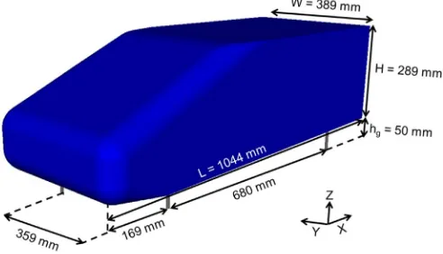
The representative bluff body used in this study is illustrated in Fig. 1. This is the square-back version of the Windsor body; a simple design which has proportions typical of a small hatch-back car and has been used in a wide range of aerodynamics studies (See, for example, Volpe et al. (2014);Littlewood et al. (2011);Littlewood and Passmore (2010);Howell et al. (2013);Howell and Le Good (2008);Howell et al. (2003)). As shown, it is 1044 mm long, 389 mm high and 289 mm wide; with a stated projected frontal area (A) of 0.112 m2.

It is usually mounted using four threaded bars (M8) at positions representative of front and rear axles, 15 mm inboard of the sides of the model. To maintain comparability with the available experimental data, ground clearance was set to 50 mm (h /H =0.17g ).

One important advantage of using standard reference geometry is that experimental data is available to support correlation with the CFD simulation. In addition to limited qualitative data for surface contam-ination deposition (Kabanovs et al., 2016), zero-yaw drag and lift coefficients are available (Perry et al., 2015) along with the rear wake topology (Pavia et al., 2016).

Hence, the representation of a key vehicle type and the availability of experimental data for both aerodynamics and surface contamination make this a good initial system for the investigation of the interaction between a tyre spray and vehicle wake.

2.2. Mathematical models

Numerical simulations were performed with a commercially avail-able CFD code, Exa PowerFLOW. This has been previously been applied to wind engineering (Mamou et al., 2008a, 2008b; Syms, 2008) as well as vehicle aerodynamics simulations (Chen et al., 2003). It is an inherently unsteady Lattice Boltzmann (LB) solver which uses what is essentially a Very Large Eddy Simulation (VLES) turbulence model (Chen et al., 1992, 1997, 2003), as when typically applied to bluffbody aerodynamics simulations the spatial resolution used is too coarse to resolve more than 80% of the turbulent kinetic energy (Pope, 2013, p.575). Unresolved turbulence is accounted for by including an effective turbulent relaxation time, calculated via the RNGκ-ε trans-port equations (Chen et al., 2003).

The discrete airborne droplets of the spray were represented via a Lagrangian particle model. This technique has been previously applied to dispersed phase simulations, such as: wind-driven rain (Hangan, 1999; Persoon et al., 2008) and sand (Paz et al., 2015); water droplets falling under gravity (Meroney, 2006); pesticide spray (Xu et al., 1998); particulate atmospheric pollutants (Ahmadi and Li, 2000) and spray from vehicle tyres (Kuthada and Cyr, 2006). In this case, the particle model was run concurrently with the LB solver. Hence particle andflow time are coupled, enabling the particles to respond to the unsteadyflow and allowing for two-way momentum transfer between the continuous and discrete phases. This has been extended to include standard models for splash (Mundo et al., 1995;O’Rourke and Amsden, 2000) and breakup (O’Rourke and Amsden, 1987). At the surface, particle mass, which is not lost via splash, is transferred into a thin surfacefilm, represented by a model similar to that ofO’Rourke & Amsden (1996). A re-entrainment model strips particles from the film if a user-set critical film thickness is exceeded. This continues until its thickness falls below a critical threshold, set at 0.3 mm in this work (Jilesen et al., 2015).

This combination of an eddy-resolving unsteadyflow solver with extended particle and surfacefilm sub-models provides a suitable tool for the investigation of the rear surface contamination problem. It is important to note that capturing the transport of droplets into a wake through the bounding shear layer requires the use of higherfidelity turbulence modelling than more widely used correlation-moment closure models provide, as these cannot capture the relevant unsteady structures in the shear (mixing) layer (Yang et al., 2004). Similarly, Paschkewitz (2006)demonstrated, while investigating the dispersion of a modelled tyre spray through the wake of a simplified lorry, that an LES turbulence model increased the vertical dispersion of the lowest inertia particles, compared to unsteady RANS (URANS). The use of LES increased the vertical dispersion distance by 35%, for particles with a diameter less than 5×10−5m. This is twice the mean diameter of the particle distribution used here; hence, the use of an unsteady eddy-resolving approach is essential.

2.3. Simulation domain

The simulation domain was designed to replicate the environment provided by the test section of the Loughborough University Wind Tunnel, as this facility was used in the equivalent experiments. The wind tunnel, described in detail byJohl et al. (2004), is a semi-open return design with a closed working section measuring 1.92 m (wide) by 1.32 m (high).

Fig. 2provides a cut-away view of the numerical domain, showing: inlet, outlet, floor and one of the two vertical walls (for the sake of clarity the ceiling and remaining vertical wall are not shown). The height and width of the working section match that of the wind tunnel, but the length of the domain has been extended both upstream and downstream to provide sufficient clearance between the bluff body, inlet and outlet. A prescribedflow velocity is set at the inlet, whilst the outlet is set to atmospheric pressure.

The floor, ceiling and wall boundary conditions are frictionless, until they reach a position 3.8 m upstream of the bluffbody, when they switch to no-slip to enable the growth of boundary layers which match that of the wind tunnel. Initial simulations without the bluff body present were used to confirm that afloor boundary layer with a 65 mm 95% disturbance thickness was attained at the centre of the working section, matching the wind tunnel. In addition, the specification of 5% turbulence intensity at the inlet resulted in a 0.15% level at the model mounting position, again matching the wind tunnel environment.

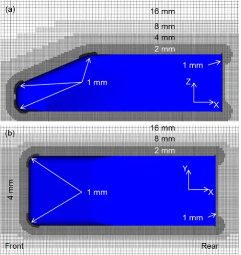
The starting point for the computational grid (lattice) design was provided by previously published studies using this LB solver (Lietz et al., 2002; Fischer et al., 2008, 2010; Samples et al., 2010). These particularly address the distribution of spatial resolution required to capture theflow structures and forces generated by automotive bodies. The chosen spatial distribution of computational cells (voxels) around the bluff body is shown inFig. 3. The individual voxels are cubes, with the smallest (1 mm) reserved for regions with the strongest pressure gradients (leading radii) and the rear face. These zones are nested within regions of reducing resolution, with 4 mm voxels used through the complete near-wake. This resulted in a computational grid (lattice) comprising 21.9×106voxels and 1.18×106 surface elements (surfels).

The level of resolution used here aligns with previously published investigations into the aerodynamics of the Ahmed body - a similar simple bluffbody - using this solver. In particular,Sims-Williams and Duncan (2003)obtained good results for the trailing vortex structures

generated by the 25° rear slant angle variant, for both time-averaged and unsteady quantities using a lattice with a smallest voxel edge length of 1.3 mm. Similarly,Fares (2006)obtained excellent results for the wake of the same Ahmed body configuration, adopting a similar disposition of spatial resolution and a smaller number of voxels (18.4×106_{) following a lattice resolution study.}

With the inlet velocity set to 30.5 m/s surface y+ values were generally below 120 for surfaces with attachedflow; appropriate for the wall model used to represent the boundary layer (Krastev and Bella, 2011). This also resulted in a Reynolds number (ReH) of 6.65×105, and

a time-step length for the simulations of 5.06×10−6s. These boundary conditions were used for both the initial aerodynamics and the subsequent surface contamination simulations.

2.4. Spray model

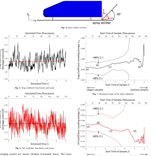
For the surface contamination simulation, the aerodynamics model was modified to include a spray source matching that used inKabanovs et al. (2016); this is illustrated inFig. 4. The spray emitter was placed on the vertical centreline (Y=0) plane at the domainfloor, immediately beneath the trailing edge of the Windsor body, with its main axis at 45° above the horizontal. Its diameter was set to 0.378 mm and particles are emitted with a velocity of 15.2 m/s. The experimental droplet size distribution was matched by a Gamma distribution with a mean particle diameter of 25.6×10−6m and a standard deviation of 15×10−6m. The conical spray had an evenly distributed angular spread (ε) of 70°. As in the experiments, water was used as the contaminant; so, appropriate material properties were set: density (ρ) 1000 kg/m3_;

dynamic viscosity (μ) 1×10−3Pa.s, and surface tension (γ) 72.8×10-3

N/m.

Clearly this experimental system is highly simplified: wheels have been omitted and the spray is introduced centrally, rather than at outboard positions, as would be the case if tyre interaction with a wet road were responsible for the spray. Neither have particle velocities been matched to those seen for droplets released from tyre surfaces. However, it does allow for the investigation of the basic process of spray transport into the base wake and the deposition of material on the rear surfacegivenits presence in the wake. The following section presents and discusses the results obtained. As a physically realistic aerodynamics simulation is a prerequisite for a credible simulation of surface contamination accumulation, these results are discussedfirst.

3. Results and discussion

3.1. Aerodynamics simulation

To establish theflowfield, an initial aerodynamic simulation was run for 6 s, requiring 4646 CPU.hours of computational effort. The drag and lift coefficients obtained are shown in Figs. 5 and 6, respectively. They are plotted against both dimensional and scaled simulated time. The latter is obtained by scaling against the time taken for the bulkflow to pass one vehicle length, i.e.L/V∞, characterising time as a number of“flow passes”. The mean values over the selected

Fig. 2.Cut-away of the computational domain.

Fig. 3.Distribution of spatial resolution.

A.P. Gaylard et al. Journal of Wind Engineering & Industrial Aerodynamics 165 (2017) 13–22

averaging period are shown (broken horizontal lines). The force coefficients have been corrected for domain (i.e. working section) blockage using the one-dimensional continuity correction ofCarr and Stapleford (1983), the same approach used inPerry et al. (2015).

Selecting the averaging period generally requires the systematic exclusion of unphysical data arising from the “start-up”phase of the simulation, where the flow field adjusts from initialisation. This is achieved by using a receding average function: a series of averages (means) is obtained for successively smaller samples by sequentially removing early-time data, e.g.:∑T_tC ND/ ,∑t tC/(N− 1),∑ C/(N− 2)…

T

D t t

T D

+∆ +2∆ ;

wheretandTare thefirst and last times, respectively, for which drag coefficient (CD) data was recorded and N is the total number of CD values in the time series. Finally,∆tis the interval for recording data (not, in this case, the simulation time step).

Receding averages are plotted for both lift and drag coefficient in Figs. 7 and 8. Confidence limits have beenestimatedaccounting for the

dependence of data points on preceding data (i.e. autocorrelation). This was realized by splitting the time series into contiguous “blocks” containing a prescribed number of points. Mean force coefficients were

Fig. 4.Spray emitter location.

Fig. 5.Drag coefficient time history and mean.

Fig. 6.Lift coefficient time history and mean.

Fig. 7.Receding average of the drag coefficients.

Fig. 8.Receding average of the lift coefficients.

Table 1

Calculated and measured force coefficients.

Drag coefficient, CD Lift coefficient, CL

CFD Experiment Δ% CFD Experiment Δ%

then calculated within each data block, providing a new time-series for which statistical quantities could be calculated. A sensitivity analysis was performed, varying the block size to determine a fair estimate for the confidence intervals.Figs. 7 and 8show confidence limits based on splitting the time series into blocks of 275 data points and calculating confidence intervals for the receding averages of this data.

For both drag and lift coefficients, removing early time data changes the mean little (a), indicating an insignificant (for the mean at least) “start-up”phase. In both cases there is a plateau (b) where the mean does not vary significantly, indicating that well-settled time-mean force coefficients have been obtained. As more data is removed and the sample size falls, the mean values show a progressive drift (c), which is more marked for the lift coefficient. Ultimately there are too few samples to obtain a stable mean (d). These observations justify the use of the complete data set to form both mean coefficients andflowfields.

This process produced mean force coefficients ofC =0.286±0.003D and C =-0.107∓0.003L (95% confidence intervals shown). These are compared with the experimental measurements ofPerry et al. (2015)in Table 1; agreement is excellent. However the base wake is critical to the rear surface contamination problem hence good prediction of the integrated force coefficients is a necessary but not a sufficient condition for a successful application of this technique.

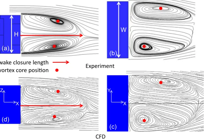
Fig. 9 re-plots Particle Image Velocimetry (PIV) measurements made byPavia et al. (2016), providing time averaged streamlines on the vertical (XZ) centreline (Y=0) and the horizontal (XY) mid-height planes; which are then compared to streamlines computed from the CFD simulation (only the rear end of the body is shown). This reveals a wake structure dominated by a ring vortex, similar to that described by Krajnović and Davidson (2003) for a bus-shaped body and later by Rouméas et al. (2009)for a simplified square-back geometry. The

time-Experiment

X Z

X Y

(b)

CFD

(c)

(d)

(a)

wake closure length

vortex core posi on

W

H

Fig. 9.Time-averaged wake structure comparison between experimental PIV data for (a) Y=0 plane and (b) Mid-Height Z Plane and CFD for (c) Y=0 plane and (d) Mid-Height Z Plane.

0.00

0.25

0.50

0.75

1.00

1.25

0.00

0.25

0.50

0.75

1.00

EXP

CFD

Heig

ht

Abov

e

W

ind

T

unnel

F

loor

,

Z

/

H

Velocity Magnitude, V

/ V

Lateral

P

osi

ti

on,

Y

/W

Velocity Magnitude, V

/ V

-0.50

-0.25

0.00

0.25

0.50

0.00

0.25

0.50

0.75

1.00

(a)

(b)

Fig. 10.Velocity magnitude one body height downstream in (a) Y=0 plane and (b) Mid-Height Z Plane. Symbols denote experimental data and solid line CFD results.

A.P. Gaylard et al. Journal of Wind Engineering & Industrial Aerodynamics 165 (2017) 13–22

averaged wake structure is well-captured by the CFD simulation. Comparing Fig. 9(a) and (d) shows the vortex core position for the lower leg of the ring vortex sitting slightly too low in the CFD simulation, due to reduced up-wash lower wake. In addition, the near wake closure occurs slightly later in the simulatedflowfield, leading to a near wake 4.5% longer than that measured. In the horizontal plane (Fig. 9(b) and (c)), the overall topology is replicated, but the vortex core location provided by the CFD simulation compares less well to experiment. This is likely a function of a lateral wake bi-stability identified for this bluffbody byPavia et al. (2016)and the smaller time-sample obtainable in CFD (6 s) against experiment (137.7 s). Thus, it is possible for the CFD simulation to be recovering the same time-dependantflowfield as experiment, but have a different mean vortex ring orientation because the run time is insufficient to capture the lateral switches inflow structure seen in the longer experiment.

Additional confirmation of the degree to which the CFD simulations recover physically realistic wake aerodynamics is provided byFig. 10,

which shows the variation of velocity magnitude (relative to the freestream velocity) at an X-location one body height (H) downstream of the base. This location was selected as it corresponds to the position of the vortex core. It is clear that the CFD simulation has captured the velocity deficit in the central part of the wake. The largest differences are seen in the y=0 plane (a) in regions of the wake affected by the upper free shear layer and theflow emerging from underneath the model.

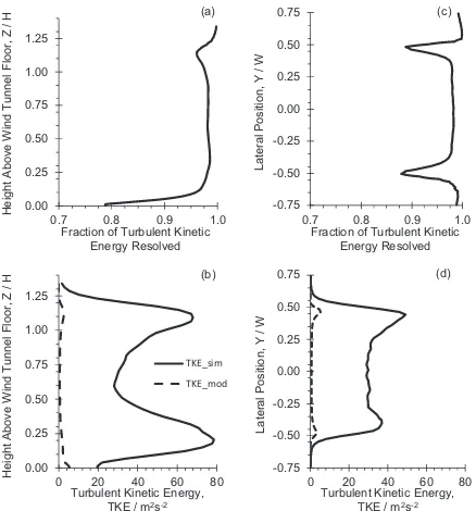
Afinal insight into the results of the aerodynamic simulation is provided inFig. 11. This plots the fraction of turbulent kinetic energy resolved in the wake (at the same downstream location) along with the distribution of the absolute values of simulated and modelled turbulent kinetic energy. This shows that the level of spatial resolution used is sufficient to resolve more than 80% of the energy through the bulk of the wakeflow.

Hence, it is clear that the CFD simulation has replicated the wake structure well and that the initial aerodynamics simulation provides a

-0.75

-0.50

-0.25

0.00

0.25

0.50

0.75

0

20

40

60

80

-0.75

-0.50

-0.25

0.00

0.25

0.50

0.75

0.7

0.8

0.9

1.0

0.00

0.25

0.50

0.75

1.00

1.25

0

20

40

60

80

TKE_sim

TKE_mod

0.00

0.25

0.50

0.75

1.00

1.25

0.7

0.8

0.9

1.0

H

/

Z

,r

o

ol

F

l

e

n

n

u

T

d

ni

W

e

v

o

b

A

t

h

gi

e

H

Fraction of Turbulent Kinetic

Energy Resolved

Lateral

P

osi

ti

o

n,

Y

/

W

(a)

(c)

H

/

Z

,r

o

ol

F

l

e

n

n

u

T

d

ni

W

e

v

o

b

A

t

h

gi

e

H

(b)

Lateral

P

osi

tion,

Y

/

W

(d)

Turbulent Kinetic Energy,

TKE / m

_s

Turbulent Kinetic Energy,

TKE / m

_s

Fraction of Turbulent Kinetic

Energy Resolved

good starting point for the surface contamination calculation.

3.2. Surface contamination simulation

3.2.1. Distribution pattern

The subsequent surface contamination simulation was run for 3.34 s of simulated time, requiring 1.01×105_{CPU.hours of}

computa-tional effort. Time-dependant particle and surface film data were

averaged to allow for comparison with the time-averaged flowfield. The predicted surface contamination distribution obtained is shown in Fig. 12(a) where it is compared to the equivalent experimental result (b).

The first point to note here is that the experimental data is a distribution of intensity (I) resulting from the use of a UVfluorescing dye in the water spray, whereas the computational image is based on

film thickness (h). Hence, although the two are related (ash∝Ifor thin

films) any comparison is qualitative and limited to the form of the distribution (to aid interpretation two broken lines have been added to

Fig. 12.Rear surface contamination pattern from (a) CFD and (b) Experiment (Kabanovs et al., 2016). Broken lines delineate subjectively assessed regions of high, medium and low surface contamination obtained in the experiment.

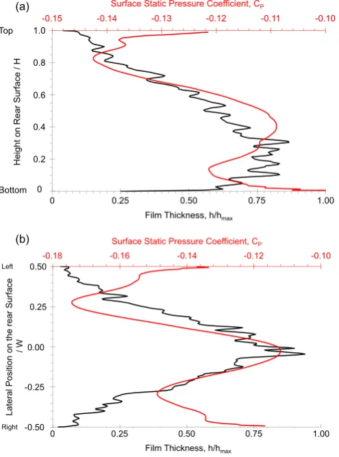
Fig. 13.Relative surfacefilm thickness and static pressure coefficient for (a) vertical centreline and (b) horizontal line through the contamination maximum the CFD simulation shows a radially distributed deposition of material, with a maximum on the vehicle centre line, at around 25% of the base height.

Fig. 14.An isosurface of water volume ratio (7.5×10-8_{) coloured by mean particle} diameter shown with streamlines on the Y=0 Plane.

Fig. 15.Rear surfacefilm mass time history.

A.P. Gaylard et al. Journal of Wind Engineering & Industrial Aerodynamics 165 (2017) 13–22

indicate the boundaries of zones of low, medium and high contamina-tion seen in the experiment).

The corners of the base are largely free of contaminant. This broadly aligns with the experimental data, particularly on the centre line where the bounds of the zones of high and moderate contamination match well. However, the experiment shows the maximum sitting lower on the base and the overall distribution spread more laterally. The latter feature is likely due to the combination of lateral wake instability seen for this geometry and longer data acquisition period available experimentally. However, the result is sufficiently credible to permit the use of the CFD to provide some insights into the processes involved.

3.2.2. Surface contamination and base pressure

A relationship between the accumulation of material on the base and the local static pressure has been asserted by Costelli (1984) following wind tunnel experiments on a small hatchback car. He observed that areas of high contamination were associated with regions of higher base pressure. This is generally borne out by the CFD simulation, as can be seen by plotting averagefilm thickness against static pressure on the vertical centreline and a horizontal plane through the deposition maximum (Fig. 13).

For inboard regions, higher base pressure is strongly associated with higher levels of surface contamination. At the edges of the base the CFD model predicts some pressure recovery, which is not matched by contaminant deposits. A consideration of the deposition mechanisms provides some explanation for this.

3.2.3. Deposition mechanisms

The basic process of deposition is illustrated inFig. 14. This plots streamlines on the vertical centreline against an isosurface of effective water volume ratio (Volume of particles/volume of voxel=7.5×10-8₎ co-loured by mean particle diameter. This shows the spray being advected downstream (a), away from the body, until the reversedflow in the lower lateral leg of the ring vortex (b) draws a fraction of the particles back towards the vehicle. The bulk of the captured particles are held in the lower part of the wake, with relatively little mixing into the upper part of the ring vortex (c). It also appears that as the contaminant approaches the rear surface it is drawn downwards by the localflow turning to align with the surface. It is notable that only a small fraction of the particles released into theflow (less than 1.0% by mass) are deposited on the rear surface.

The retention of the largest fraction of particles in the lower part of the wake explains the position of the contamination maximum on the rear surface. Its association with the returnflow and subsequent rear stagnation point explains the relationship with regions of high base pressure suggested byCostelli (1984)and seen inFig. 13. The deviation noted from this association approaching the lower trailing edge appears to be caused by local downwash in theflowfield. Those seen approaching the upper and body side edges are caused by the relative lack of contaminant in proximity to the rear surface in these areas.

The simulation also suggests that the main transport mechanism of contaminant to the rear surface is theflow reversal associated with the lower part of the ring vortex. Few particles appear to penetrate the lower shear layer. In addition, the distribution of mean particle diameter over the isosurface indicates that the process of turning the particles leads to break-up, as the fraction of large particles decreases as they approach the rear surface.

3.2.4. Rate of accumulation

Thefinal set of observations provided in this work relate to the rate of accumulation of material on the rear surface. The time histories of

film mass and its rate of deposition are provided inFigs. 15 and 16, respectively.

FromFig. 15it is clear that over the period simulated, the film accumulates linearly, with5.65 ×10 kg-5 _{of the dispersed phase} depos-ited on the rear surface over the course of the simulation. The linear trend aligns with simulations conducted for a fully-detailed road vehicle byJilesen et al. (2013), suggesting that the insights provided by this simple system are relevant to actual vehicles.

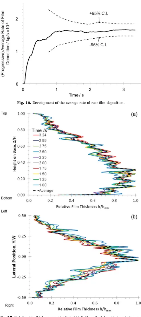
The reason for the linear accumulation of mass on the rear surface is provided inFig. 16. This plots the time-history of the progressive average (i.e. the start of the averaging window remainsfixed, with new data added sequentially) of the deposition rate (solid line), along with the bounds for a 95% confidence interval (broken lines). As can be seen, the rate of deposition reaches a well-settled mean value after one second of simulated time. From then on the average rate remains largely constant, reaching afinal value of(1.7 ± 0.2) ×10 kg/s-5 _{; only} 1.0% of the rate input into the simulation.

Fig. 16.Development of the average rate of rearfilm deposition.

These observations indicate that although longer simulations will generate a thicker film (up to the point where the surface cannot support the liquid against gravity and aerodynamic shear, leading to

film run-off) the form of the distribution is likely to remain unchanged. This view is confirmed by the time-series of relative film thickness profiles (i.e. film height divided by the maximum value along the profile) presented in Fig. 17. These show relative film thickness distribution on the (a) vertical centreline and (b) a horizontal plane through the contamination maximum. The individual profiles are similar over the time period shown, with differences diminishing as the simulation progresses. This provides good evidence that although

film thickness increases over time, the relative distribution does not. Hence, comparisons of relative distributions between relatively short CFD calculations and longer experiments may be warranted.

4. Conclusions

An extended LB solver has been shown to provide an excellent representation of the aerodynamics of a simple square-backed bluff body, leading to a credible prediction of the relative distribution of contaminant on the rear surface. Thus the potential of this eddy-resolving method to predict these important characteristics is demon-strated.

Deposition of surface contaminant on the rear surface of a representative bluff body has been shown to be the result of spray entrainment by the lower part of the wake ring vortex. Relatively little material appears to be advected across the lower shear layer.

Surface contaminant accumulates preferentially in regions of higher base pressure, as suggested byCostelli (1984). Exceptions to this trend are seen (a) close to the lower edge of the base, due to local wake downwash and (b) close to the remaining edges, due to low local availability of contaminant.

In this simulation, the fraction of emitted material deposited on the rear surface was small, only 1.0% of the total mass of contaminant introduced into the domain.

In common with actual vehicles, the accumulation of contaminant is linear, with the deposition rate and relative distribution changing little over time. This suggests that shorter CFD simulations can be compared to longer experiments. It also suggests that the rate of accumulation is a useful metric for future studies, as is constant and usefully related to vehicle development objectives: i.e. vehicles oper-ated in the environment will always accumulate contaminant, but reducing the rate at which this occurs can help differentiate between designs.

Finally, for real vehicles, the source of surface contamination is spray generated by tyres lifting water containing solid contaminants from wet road surfaces. Also, the wheels generate their own wake structure. These elements have been omitted from this study, so the next stage in the systematic application of simplified vehicle geometries to this problem should be based around a standard body which incorporates wheels.

Acknowledgements

The authors would like to thank Giancarlo Pavia (Loughborough University) for re-plotting PIV data fromPavia et al. (2016)to facilitate direct comparison with the CFD simulation presented here, and Dr Anna-Kristina Perry (Loughborough University) for providing the additional experimental data used inFig. 10.

The work of A. P. Gaylard and A. Kabanovs is supported by Jaguar L and Rover and the UK-EPSRC grant EP/K014102/1 as part of the jointly funded Programme for Simulation Innovation.

D. A. Lockerby's time has been financially supported by EPSRC grants EP/N016602/1, EP/K038664/1 and EP/I011927/1.

References

Ahmadi, G., Li, A., 2000. Computer simulation of particle transport and deposition near a small isolated building. J. Wind Eng. Ind. Aerodyn. 84 (1), 23–46.http://dx.doi.org/ 10.1016/S0167-6105(99)00048-3.

Carr, G. W., Stapleford, W. R. (1983). Blockage Effects in Automotive Wind-Tunnel Testing. SAE Technical Paper 860093. In: Proceedings of the SAE International Congress and Exposition, February 24–28, 1986, Detroit, MI, USA. Warrendale: Society of Automotive Engineers, Inc. DOI:10.4271/860093.

Chen, H., Chen, S., Matthaeus, W.H., 1992. Recovery of the Navier-Stokes equations using a lattice-gas Boltzmann method. Phys. Rev. A 45 (8), R5339–R5342.http:// dx.doi.org/10.1103/PhysRevA.45.R5339.

Chen, H., Teixeira, C., Molvig, K., 1997. Digital physics approach to computationalfluid dynamics: some basic theoretical features. Int. J. Mod. Phys. C 8 (4), 675–684.

http://dx.doi.org/10.1142/S0129183197000576.

Chen, H., Kandasamy, S., Orszag, S., Shock, R., et al., 2003. Extended Boltzmann kinetic equation for turbulentflows. Science 301 (5633), 633–636.http://dx.doi.org/ 10.1126/science.1085048.

Costelli, A. F. (1984). Aerodynamic Characteristics of the Fiat UNO Car. SAE Technical Paper 840297. In: Proceedings of the SAE 1984 International Congress & Exposition, Detroit, February 27–March 2 1984. Warrendale: SAE International. doi:10.4271/840297.

Fares, E., 2006. Unsteadyflow simulation of the Ahmed reference body using a lattice Boltzmann approach. Comput. Fluids 35 (8–9), 40–95.http://dx.doi.org/10.1016/ j.compfluid.2005.04.011.

Fischer, O., Kuthada, T., Mercker, E., Wiedemann, J. et al., (2010). CFD Approach to Evaluate Wind-Tunnel and Model Setup Effects on Aerodynamic Drag and Lift for Detailed Vehicles. SAE Technical Paper 2010-01-0760. In: Proceedings of the SAE 2010 World Congress, April 13–15,Detroit, MI, USA. Warrendale: SAE International. DOI:10.4271/2010-01-0760.

Fischer, O., Kuthada, T., Wiedemann, J., Dethioux, P. et al. (2008). CFD Validation Study for a Sedan Scale Model in an Open Jet Wind Tunnel. SAE Technical Paper 2008-01-0325. In: Proceedings of the SAE 2010 World Congress, April 14–17,Detroit, MI, USA. Warrendale: SAE International. DOI:10.4271/2008-01-0325.

Gaylard, A., Pitman, J., Jilesen, J., Gagliardi, A., et al., 2014. Insights into Rear Surface Contamination Using Simulation of Road Spray and Aerodynamics. SAE Int. J. Passeng. Cars - Mech. Syst.7 (2), 673–681. http://dx.doi.org/10.4271/2014-01-0610.

Hangan, H., 1999. Wind-driven rain studies. A C-FD-E approach. J. Wind Eng. Ind. Aerodyn. 81 (1–3), 323–331.http://dx.doi.org/10.1016/S0167-6105(99)00027-6. Howell, J., Passmore, M., Tuplin, S., 2013. Aerodynamic drag reduction on a simple

car-like shape with rear upper body taper. SAE Int. J. Passeng. Cars - Mech. Syst. 6 (1), 52–60.http://dx.doi.org/10.4271/2013-01-0462.

Howell, J., Sheppard, A., Blakemore, A. (2003). Aerodynamic Drag Reduction for a Simple BluffBody Using Base Bleed. SAE Technical Paper 2003-01-0995. In: Proceedings of the SAE 2003 World Congress, March 3–6,Detroit, MI, USA. Warrendale: SAE International. DOI:10.4271/2003-01-0995.

Howell, J., Le Good, G., (2008). The Effect of Backlight Aspect Ratio on Vortex and Base Drag for a Simple Car-Like Shape. SAE Technical Paper 2008-01-0737. In: Proceedings of the SAE 2008 World Congress, April 14–17,Detroit, MI, USA. Warrendale: SAE International. DOI:10.4271/2008-01-0737.

Hu, X., Liao, L., Lei, Y., Yang, H., et al., 2015. A numerical simulation of wheel spray for simplified vehicle model based on discrete phase method. Adv. Mech. Eng. 7 (7), 1–8 .http://dx.doi.org/10.1177/1687814015597190.

Jilesen, J., Alajbegovic, A., Duncan, B., 2015. Soiling and Rain Simulation for Ground Transportation. In: Proceedings of the 7th European-Japanese Two-Phase Flow Group Meeting (7TH-EUJPTPFGM 2015), 11-15 October 2015, Zermatt, Switzerland.

Jilesen, J., Gaylard, A., Duncan, B., Konstantinov, A., et al., 2013. Simulation of rear and body side vehicle soiling by road sprays using transient particle tracking. SAE Int. J. Passeng. Cars - Mech. Syst. 6 (1), 424–435. http://dx.doi.org/10.4271/2013-01-1256.

Johl, G., Passmore, M., Render, P., 2004. Design methodology and performance of an indraft wind tunnel. Aeronaut. J. 108 (1087), 465–473.

Kabanovs, A., Varney, M., Garmory, A., Passmore, M. et al. (2016). Experimental and Computational Study of Vehicle Soiling on a Generic Hatchback Body. SAE Technical Paper 2016-01-1604. In: Proceedings of the SAE 2016 World Congress and Exhibition, April 12–14, Detroit, MI, USA. Warrendale: SAE International. DOI:10. 4271/2016-01-1604.

Krajnović, S., Davidson, L., 2003. Numerical study of theflow around a bus-shaped body. J. Fluids Eng. 125 (3), 500–509.http://dx.doi.org/10.1115/1.1567305. Krastev, V., Bella, G. (2011). On the Steady and Unsteady Turbulence Modeling in

Ground Vehicle Aerodynamic Design and Optimization. SAE Technical Paper 2011-24-0163. In: Proceedings of the ICE2011 - 10th International Conference on Engines & Vehicles, September 11–15, 2011, Capri, Napoli, Italy. Warrendale: SAE International. DOI:10.4271/2011-24-0163.

Kuthada, T., Cyr, S., 2006. Approaches to vehicle soiling. In: Wiedermann, J., Hucho, W.H. (Eds.), Progress in Vehicle Aerodynamics, IV, Numerical methods. Expert-Verlag, Renningen, 111–123.

Lajos, T., Preszler, L., Finta, L., 1986. Effect of moving ground simulation on theflow past bus models. J. Wind Eng. Ind. Aerodyn. 22 (2), 271–277.http://dx.doi.org/ 10.1016/0167-6105(86)90090-5.

Le Good, G., Garry, K., (2004). On the Use of Reference Models in Automotive Aerodynamics. SAE Technical Paper 2004-01-1308. In: Proceedings of the SAE 2004 World Congress, March 8–11, 2004, Detroit, MI, USA. Warrendale: SAE

A.P. Gaylard et al. Journal of Wind Engineering & Industrial Aerodynamics 165 (2017) 13–22

International. DOI:10.4271/2004-01-1308.

Lietz, R., Mallick, S., Kandasamy, S., Chen, H (2002). Exterior Airflow Simulations Using a Lattice Boltzmann Approach. SAE Technical Paper 2002-01-0596. In: Proceedings of the SAE 2002 World Congress, March 4–7, 2002, Detroit, MI, USA. Warrendale: SAE International. DOI:10.4271/2002-01-0596.

Littlewood, R., Passmore, M., Wood, D., 2011. An investigation into the wake structure of square back vehicles and the Effect of structure modification on resultant vehicle forces. SAE Int. J. Engines 4 (2), 2629–2637. http://dx.doi.org/10.4271/2011-37-0015.

Littlewood, R., Passmore, M. (2010). The Optimization of Roof Trailing Edge Geometry of a Simple Square-Back. SAE Technical Paper 2010-01-0510, In: Proceedings of the SAE 2010 World Congress, April 13–15, 2010, Detroit, MI, USA. Warrendale: SAE International. DOI:10.4271/2010-01-0510.

Mamou, M., Cooper, K.R., Benmeddour, A., Khalid, M., et al., 2008b. Correlation of CFD predictions and wind tunnel measurements of mean and unsteady wind loads on a large optical telescope. J. Wind Eng. Ind. Aerodyn. 96 (6–7), 793–806.http:// dx.doi.org/10.1016/j.jweia.2007.06.050.

Mamou, M., Tahi, A., Benmeddour, A., Cooper, K.R., Abdallah, I., et al., 2008a. Computationalfluid dynamics simulations and wind tunnel measurements of unsteady wind loads on a scaled model of a very large optical telescope: a comparative study. J. Wind Eng. Ind. Aerodyn. 96 (2), 257–288.http://dx.doi.org/ 10.1016/j.jweia.2007.06.002.

Maycock, G. (1966). The problem of water thrown up by vehicles on wet roads. Harmondsworth: Road Research Laboratory. (LR4).

Meroney, R.N., 2006. CFD prediction of cooling tower drift. J. Wind Eng. Ind. Aerodyn. 94 (6), 463–490.http://dx.doi.org/10.1016/j.jweia.2006.01.015.

Mundo, C., Sommerfeld, M., Tropea, C., 1995. Droplet-wall collisions: experimental studies of the deformation and breakup process. Int. J. Multiph. Flow. 21 (2), 151–173.http://dx.doi.org/10.1016/0301-9322(94)00069-V.

O'Rourke, P., Amsden, A. (1987). The TAB Method for Numerical Calculation of Spray Droplet Breakup. SAE Technical Paper 872089. In: Proceedings of the International Fuels and Lubricants Meeting and Exposition, Toronto, Ontario, November 2–5, 1987. Warrendale: The Society of Automotive Engineers, Inc. DOI:10.4271/872089. O'Rourke, P., Amsden, A. (2000). A Spray/Wall Interaction Submodel for the KIVA-3

Wall Film Model. SAE Technical Paper 2000-01-0271. In: Proceedings of the SAE 2000 World Congress, March 6–9, 2000, Detroit, MI, USA. Warrendale: SAE International. DOI:10.4271/2000-01-0271.

O'Rourke, P., Amsden, A. (1996). A Particle Numerical Model for Wall Film Dynamics in Port-Injected Engines. SAE Technical Paper 961961. In: Proceedings of the International Fall Fuels & Lubricants Meeting & Exposition, San Antonio, Texas, October 14–17, 1996. Warrendale: Society of Automotive Engineers, Inc.DOI:10.

4271/961961.

Paschkewitz, J. S. (2006). A comparison of dispersion calculations in bluffbody wakes using LES and unsteady RANS. United States: Lawrence Livermore National Laboratory. (UCRL-TR-218576). )〈https://e-reports-ext.llnl.gov/pdf/329543.pdf〉. Pavia, G., Passmore, M., Gaylard, A. (2016). Influence of Short Rear End Tapers on the

Unsteady Base Pressure of a Simplified Ground Vehicle. SAE Technical Paper 2016-01-1590. In: Proceedings of the SAE 2016 World Congress and Exhibition, April 12– 14, Detroit, MI, USA. Warrendale: SAE International. DOI:10.4271/2016-01-1590. Paz, C., Suárez, E., Gil, C., Concheiro, M., 2015. Numerical study of the impact of

windblown sand particles on a high-speed train. J. Wind Eng. Ind.Aerodyn. 145, 87–93.http://dx.doi.org/10.1016/j.jweia.2015.06.008.

Perry, A., Passmore, M., Finney, A., 2015. Influence of short rear end tapers on the base pressure of a simplified vehicle. SAE Int. J. Passeng. Cars - Mech. Syst. 8 (1), 317–327.http://dx.doi.org/10.4271/2015-01-1560.

Persoon, J., van Hooff, T., Blocken, B., Carmeliet, J., et al., 2008. On the impact of roof geometry on rain shelter in football stadia. J. Wind Eng. Ind. Aerodyn.96 (8–9), 1274–1293.http://dx.doi.org/10.1016/j.jweia.2008.02.036.

Pope, S.B., 2013. Turbulent Flows. Cambridge University Press, Cambridge, UK. Rouméas, M., Gilliéron, P., Kourta, A., 2009. Analysis and control of the near-wakeflow

over a square-back geometry. Comput. Fluids 38 (1), 60–70.http://dx.doi.org/ 10.1016/j.compfluid.2008.01.009.

Samples M., Gaylard A.P., Windsor S., 2010. The aerodynamic development of the Range Rover Evoque. In: Proceedings of the 8th MIRA International Conference on Vehicle Aerodynamics, 13-14 October 2010, Grove, Oxfordshire. Nuneaton: MIRA Ltd, pp. 380–388.

Sims-Williams, D., Duncan, B. (2003). The Ahmed Model Unsteady Wake: Experimental and Computational Analyses. SAE Technical Paper 2003-01-1315. In: Proceedings of the SAE 2003 World Congress, March 3–6, Detroit, MI, USA. Warrendale: SAE International. DOI:10.4271/2003-01-1315.

Syms, G.F., 2008. Simulation of simplified-frigate airwakes using a lattice-Boltzmann method. J. Wind Eng. Ind. Aerodyn.96 (6–7), 1197–1206.http://dx.doi.org/ 10.1016/j.jweia.2007.06.040.

Volpe, R., Ferrand, V., Da Silva, A., Le Moyne, L., 2014. Forces andflow structures evolution on a car body in a sudden crosswind. J. Wind Eng. Ind. Aerodyn. 128, 114–125.http://dx.doi.org/10.1016/j.jweia.2014.03.006.

Xu, Z.G., Walklate, P.J., Rigby, S.G., Richardson, G.M., 1998. Stochastic modelling of turbulent spray dispersion in the near-field of orchard sprayers.J. Wind Eng. Ind.

Aerodyn. 74–76, 295–304.http://dx.doi.org/10.1016/S0167-6105(98)00026-9. Yang, W.B., Zhang, H.Q., Chan, C.K., Lin, W.Y., 2004. Large eddy simulation of mixing