Reducing UPPAAL models through control flow analysis

(1)

REDUCING UPPAAL

MODELS THROUGH

CONTROL FLOW ANALYSIS

G.H. Slomp

COMPUTER SCIENCE FORMAL METHODS & TOOLS

EXAMINATION COMMITTEE

(2)

Abstract

This paper present a dead variable analysis algorithm for reducing the state space of UPPAAL models. By resetting irrelevant variables to their initial value reductions of UPPAAL models are achieved.

The developed algorithm consists of two parts. In the first part we define an algorithm to determine the relevance of variables. We also cope with the various features of UPPAAL like, for instance, function calls and value passing variables and we present an algorithm to determine the relevance of variables that are used in a property. In the second part we transform the original timed au-tomata by introducing resets for irrelevant variables. We improve on extending transformation algorithms by not resetting irrelevant variables at every location. Based on the developed algorithm we implemented a tool that performs the transformation and by executing this tool for three case studies we show that it indeed achieves reductions.

(3)

CHAPTER 1

Introduction

Model checking has its roots in the 1970’s, when Computer Science was facing the problem of Concurrent Program Verification [10]. Errors in concurrent pro-grams were hard to reproduce due to the concurrency in the propro-grams. Model checking solved this problem because it offered the possibility to exhaustively search all possible execution paths within a program. A simple definition of model checking is:

”Given a modelM and a formulaϕ, model checking is the problem of verifying

whether or notϕis true inM (writtenM |=ϕ).”

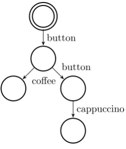
One way to represent a system as a model is by using automata, which have the advantage that besides the formal definition they can also be represented graphically. For instance, look at the automaton in figure 1.1, modelling the behaviour of a simple coffee machine. The automaton represent a coffee machine that delivers coffee after pressing the button once, but delivers cappuccino after pressing the button twice.

button

coffee

button

[image:5.595.232.359.515.665.2]

cappuccino

(6)

Having this model of figure 1.1 we want to know if the corresponding coffee machine is working properly and that it is, for example, guaranteed that you will get a cup of cappuccino if you press the button twice and do not end up with a cup of coffee. This property can be expressed in computational tree logic

(CTL) as: button.button⇒cappuccino.

The property is satisfied and we could say that the machine is working correctly. But what if somebody presses the button and an hour later someone else presses the button. In practice, after the first time the button is pressed a cup of coffee is produced and the counting starts again, but in theory this does not hold. What we actually would want is that we can say something about the time that has progressed after the button is pressed for the first time.

This is exactly what researchers encountered when they wanted to check more complex systems as for real-time systems the standard automata were not suffi-cient because a notion of time was required. Therefore, to model the behaviour of real time systems, Alur and Dill extended standard automata with clocks,

timing constraints and clock resets, resulting in timed automata [2]. Based on

these timed automata various tools were developed, which can be used in the verification of real-time systems. Two well-known examples are Kronos [13] and UPPAAL [25]. In this research we will focus on UPPAAL, a tool developed by Uppsala University, Sweden and Aalborg University, Denmark. We have chosen for UPPAAL as it is the most-used tool for modelling real timed systems.

Originally UPPAAL was based on timed automata only, but since the newer ver-sions, it uses a combined approach, also supporting imperative code. This gives users the possibility to define, for instance, functions and call these functions from the automata [4]. It has been used in various real-life problems. For in-stance, an error in an audio/video protocol by Bang & Olufsen has been found and the corrected protocol has (partially) been proven correct [17]. Another example is the analysis of the Philips Audio Control Protocol using UPPAAL [6]. Both case studies are relatively large and in both cases it takes UPPAAL several minutes to generate an error trace or prove the modelled protocol correct.

(7)

1.1

Initial exploration

As mentioned, research by van de Pol and Timmer [30] suggests that it is worth trying to adapt and apply their method on models defined in UPPAAL. The following will give an introductory view of possible reductions.

s5 s3

s2

s6

s4 s1

a=i

i : int[0,9]

a<5 a>=5

(a) Original model

s5 s2

s3 s4

s6 s1

a=0 a=0 a=i

a<5 a>=5

i : int[0,9]

[image:7.595.187.407.214.322.2]

(b) Optimised model

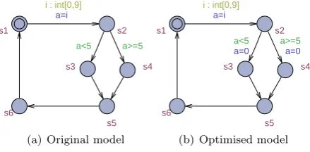
Figure 1.2: Basic example showing the possible reductions (data variables)

File States explored States stored

Before 50 50

[image:7.595.200.392.377.416.2]

After 15 15

Table 1.1: Results of the verification

In UPPAAL there are two types of variables which both seem to be suitable for control flow reconstruction in order to reduce the state space. (Discrete) data variables are the first type of variables, both global and local. Figure 1.2(a) shows a relatively simple model, which selects a value of zero to nine

and assigns the value to a variable a (see section 2 for a introduction to the

UPPAAL language or section 3 for a formal description). This variable a is

then used in the (guard of the) next edge, but, after that, is not used any more

till it is assigned a random value again. The value ofais only relevant in state

s2, while in the other states it is only a cause of a growth in the number of

states stored. By resetting the value ofain the transition froms2 tos3 ors4,

see figure 1.2(b), a reduction in the state space can be achieved. To test the

reduction we check a simple property A2x≥0 ,which is always true, in order

to compare the number of states explored/stored. Using no space optimisation we get the results as shown in table 1.1 If we take a look at the second type of variable, clock variables, the first impression is that there are less possibilities to reduce the state space. The reason for this is the fact that the clocks are

stored using zones [8]. For a data variable x, which can have values ranging

from 0–9, for every location there can be up to 10 different states just varying

in the value of x. However, a clock variable c will be stored in a state using a

zone 0≤c≤9 and therefore resetting its value does not automatically reduce

(8)

is not the case as UPPAAL only generates 4 states, where you would expect

different states for the 4 zones ; c≥0, c≥1, c≥2, resulting in 16 states. The

conclusion is that for clock variables we probably cannot reduce the state space that much (due to the clock zones), but for data variables there are certainly some reductions possible.

c=0 c=1 c=2

c<=1

Figure 1.3: Model with a state space of only four states

1.2

Research Questions

After the initial exploration we now define the research question of the project: ‘What can control flow analysis applied to UPPAAL models achieve?’. To an-swer this question we anan-swer the following sub questions:

• Can the algorithm of [30] be translated to reduce the state space of

UP-PAAL models by resetting local variables?

• Is there a way to reduce the state space by resetting global variables

without constructing the total state space?

• How can the algorithm be extended to include the state invariants of

UPPAAL?

• How can we incorporate the ’different’ features of UPPAAL into the

algo-rithm?

• Is the tool beneficial for end users of UPPAAL, releasing them from

(9)

CHAPTER 2

Related work

For a good understanding of the following sections a basic knowledge of (timed) automata is required. We give a complete formal description in section 3, but for now a short informal description is sufficient. In figure 2.1 a simple on/off switch is modelled. The circles represent the states/nodes of the automaton and the arrows between states represent the edges or transitions of the system. The

automaton of figure 2.1 starts in theOFF state (indicated by the double circle)

and can go to theON state by processing aPushaction. Once in theON state

anotherPush action moves the automaton back to theOFF state.

OF F ON

Push

[image:9.595.238.357.422.481.2]

Push

Figure 2.1: Automaton representing an on/off switch

A simple extension of the above are theguards. A guard is a boolean expression

that ‘guards’ the transition and needs to evaluate totrue for the transition to

be enabled. If a guard evaluates to f alse the transition is not enabled and

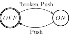
cannot be taken. If we add a boolean variable broken (initially f alse) to the

automaton of figure 2.1 and a guard !brokento the transitionOF F −−−→P ush ON

we get the automaton of figure 2.2, which does not allow the transition to be taken if the switch is broken.

OF F ON

!broken Push

Push

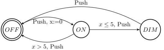
[image:9.595.239.355.625.686.2]

(10)

A great variety of systems can be modelled with the above automata, but how do we model for instance a dimmer which can be turned on by pushing the button once and can be put in dimmed state by pushing the button again in at most 5 seconds? For this problem (and other problems) a notion of time has

been added to automata to gettimed automata [2]. In figure 2.3 the dimmer is

presented as an automaton using a real-valued clock xwhich can be reset to 0.

If the automaton receives a firstP ushthe clockxis reset to measure the passed

time since theP ush. If anotherP ushoccurs within 5 seconds the transition to

DIM will be taken, otherwise the dimmer is turnedOF F.

OF F ON DIM

Push, x:=0

x >5, Push

x≤5, Push

[image:10.595.164.433.248.330.2]

Push

Figure 2.3: Automaton representing a dimmer

In section 1 we mentioned UPPAAL, a model checker for real-timed systems, which can be used to model and verify these timed automata. We also noted that UPPAAL, like model checkers in general, suffers from the state space ex-plosion problem. There are various approaches to solve this problem, which we present in the following sections. We first give an overview in section 2.1 of various techniques to reduce the size of the generated state space, followed by a description of some compiler optimisation techniques.

2.1

Reduction techniques

The following sections give an overview of the various reduction techniques that are available. We conclude with mentioning for each technique if its available in UPPAAL and automatically enabled.

2.1.1

Symmetry Reduction

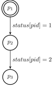
Symmetry reduction is one of the techniques to reduce the number of states to be explored and is available in UPPAAL since UPPAAL 4.0 [19, 4]. It applies the idea of symmetry reduction of Ip and Dill [21] to UPPAAL and uses the occurrence of multiple identical processes only differing in the their identity, also called full symmetry [21]. By defining an equivalence group, based on an automorphism, large reductions in the verification process can be achieved. To implement symmetry reduction two problems should be solved, the problem of detecting the automorphism from the system description and the problem of deciding the symmetry of two states during verification. Therefore the data type

(11)

under permutation of the elements of the scalar-set. For scalar-sets of size n

reductions of up to a factorn! can be achieved.

p1

p2

p3

status[pid] = 1

[image:11.595.251.337.162.306.2]

status[pid] = 2

Figure 2.4: Automaton of a processP keeping track of his status

For example consider the process in figure 2.4, which only keeps track of the current status of the process using an array called status. In the first transition

the process sets his status to 1 using the variablepid as index and in the next

transition the status is set to 2. If we have multiple of these processes, for instance two, we will get the state space of figure 2.5, which is made of all possible interleavings of the two processes. A non-dashed edge is a transition of the first process, while a dashed edge is a transition of the second process. Notice the complete symmetry of the automaton. Symmetry reduction makes use of the symmetry by exploring only a part of the total state space, which is the set of filled nodes in figure 2.5. Observe that all the non-filled nodes have an corresponding filled node only differing in (the order of) their pid’s. For

example (0,2)≡(2,0), or in general (i, j)≡(j, i).

0,0

1,0

2,0

2,1

0,1

0,2 1,1

1,2

2,2

[image:11.595.223.370.506.655.2]

(12)

2.1.2

Slicing

Another method is that ofslicing, an abstraction technique. Abstraction

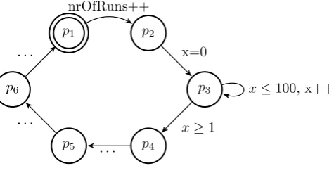
tech-niques use a part, an abstraction, of the model, in order to verify a property for the whole model. Because only a part of the model is verified the state space that needs to be generated is much smaller. However one has to make sure the abstraction preserves the properties that are verified, otherwise a correct abstraction does not guarantee the correctness of the whole model. In [22] a first approach is presented using slicing with timed automata, while in [29] it is showed how slicing can be used in the current version of UPPAAL, which uses not solely timed automata any more but is extended with new data types and user defined functions. Slicing reduces the original model to a set of relevant components with regards to some slicing criteria. These criteria are based on the locations and variables of the property to be verified. Figure 2.6 gives an

example of an abstraction slicing produces. We define a property ‘∀2not

dead-lock’, which guarantees us that the process will never deadlock. If we verify this property the statement ‘nrOfRuns++’ is irrelevant as it does not affect the control flow or another variable but serves as a status variable. The slicing al-gorithm will remove this statement from the specification and the result is that in the total state space the size of each state vector is smaller.

p1 p2

p3

p4 p5

p6

nrOfRuns++

x=0

x≥1

x≤100, x++

. . . . . .

[image:12.595.178.416.374.497.2]

. . .

Figure 2.6: Example explaining the slicing algorithm

2.1.3

Partial order reduction

A well known method to reduce the state space ispartial order reduction.

Nor-mally the next state to be explored is chosen from enabled(s), all transitions

that are enabled/possible in the state s. Partial order reduction tries to use a

setample(s)⊆enabled(s) instead [26]. If one can define a setample(s) smaller

than enabled(s) the resulting state space will be smaller. The set ample(s) is

generated by looking at the the interleaving of independent edges (transitions).

Two edgesαandβ are independent if:

• α∈enabled(β(s)) andβ∈enabled(α(s)) - They do not disable each other

(13)

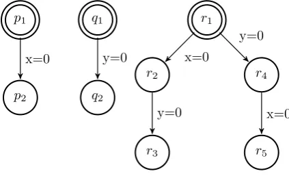
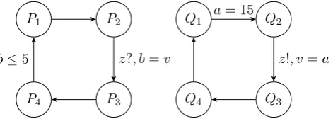
Because these edges are independent it does not matter in which order they are traversed and as a consequence it is beneficial to only traverse one possible in-terleaving of those edges. In the area of timed automata partial order reduction is a little harder because there the interleaving of, for instance, two clock resets leads to two different states and does not produce the nice diamond structure known in partial order reduction. Looking at figure 2.7 one has 2 processes with

one clock each. If, in the combined automata, xis reset first and in the next

transitionyone ends up in a state (r3) wherex≥yholds whereas the other way

around one ends in a state (r5) wherex≤y holds, whereas, in the case of data

variables statesr3 andr5 would be the same. To apply partial order reduction

to timed automata the idea of letting the local clocks proceed independently of the clocks of other processes is presented [7]. This means that whenever a synchronised action is performed the local clocks still need to be synchronised and therefore extra clocks are added to each process. A prototype has been implemented but this implementation does not show large reductions, mostly because of the introduction of a large number of extra local clocks [3].

p1

p2

q1

q2

r2

r1

r3

r4

r5 y=0

x=0 x=0

y=0

[image:13.595.188.400.329.459.2]

x=0

Figure 2.7: Interleaving two clock resets

2.1.4

Dead variable analysis

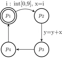
In figure 2.8 a simple automaton is presented. In this automaton a random value

(ranging from 0 to 9) is assigned toxand in the next transition this valuexis

added to the value of y. In the next two transitions the variablexis not used

and then the loop starts again andxis assigned a new random value. Because

the value ofxis not used inp3andp4and there does not exist a path to another

state wherexis used, we say thatxis not relevant inp3andp4. The other way

around we can see thatxis relevant inp2 asxis used in a outgoing transition

from p2. We can say xis relevant in p3. To reduce the state space we could

reset a variable if it is not relevant. This analysis of relevant variables is called dead (or live) variable analysis.

(14)

processes, the algorithm first tries to reduce the processes separately, without looking at the specification of a parallel process, before composing the combi-nation of all the parallel processes. Also [?] and [30] (for LPEs) present work on dead variable analysis and even the tutorial on UPPAAL [5] references dead variable analysis and gives modelling tips how to manually apply the analysis to reduce the state space. However the analysis is not integrated into UPPAAL and therefore not automatically performed.

p1 p2

p3 p4

i : int[0,9], x=i

[image:14.595.242.348.223.326.2]

y=y+x

Figure 2.8: Trivial example to demonstrate dead variable analysis

2.1.5

Exact (clock) acceleration

Hendriks and Larsen address the problem of unnecessary fragmentation of the state space, due to different time scales in the real time system [18]. This occurs, for example, when a systems samples the environment many times each second, whereas the environment only changes a couple of times each second. In a automata this can be seen as a cycle which can only be left if a clock reaches a certain value, however in the meantime the cycle is repeated many times, resulting in a very large state space because non of these iterations of the cycle

overlap. They propose an algorithm, calledexact acceleration, to transform this

cycle such that there is a new cycle which will only be traversed once resulting in a much smaller state space.

2.1.6

Active clock reduction

(15)

2.1.7

Reduction techniques in UPPAAL

In table 2.1 we indicate for each of the reduction techniques if it is implemented in UPPAAL and if it’s automatically enabled in UPPAAL. Below the table we give some remarks on the entries of the table.

Technique In UPPAAL? Automatically enabled?

Symmetry Reduction + +- (1)

Slicing - (2)

-Partial order reduction - (2)

-Dead variable analysis - (3)

-Exact clock acceleration - (2)

-Active clock reduction + +

Table 2.1: Overview of reduction techniques

1. For symmetry reduction you have to annotate an integer range as a scalar set if it is fully symmetric. If you do this the verification automatically applies symmetry reduction.

2. For all of these techniques tools/prototypes have been implemented, but there is not a complete working implementation available in UPPAAL of these techniques.

3. One of the results of this paper is a tool that can perform dead variable analysis for UPPAAL models. It is not implemented in UPPAAL but is available as an preprocessing tool.

2.2

Compiler optimisation techniques

All the methods described in the previous section are all about optimising the model checking process. However there are other research areas that have op-timisation techniques. Those techniques may be interesting for our project as they can prove useful. One interesting area is the area of compiler optimisation. Almost every compiler nowadays makes use of the Single Static Assignment form which we present first, followed by various compiler optimisation techniques of which some may prove useful for our project.

2.2.1

Static Single Assignment form

Static single assignment (SSA) [11] form is not an optimisation itself, however it is an special representation of the original code that makes it possible that other algorithms/techniques, that do cause optimisations, can be easily applied. Basically a program is in SSA form if each variable is a target of exactly one assignment statement. Using SSA form it is easier to see which variable assign-ment corresponds to a particular use of a variable. Consider the following piece of code:

y:= 1

y:= 2

(16)

It is easy to see that the first assignment has no use as the value it assigns will never be used, but one can imagine this will be harder when the code gets more complex. Even for this small piece of code it is clear that SSA form makes it easier to draw conclusions about the use of variables. To translate the piece of code we assign to every variable an unique (for that variable) index number. Each use of a variable will get the same index number as the corresponding definition of that variable. For the example this results in:

y1:= 1

y2:= 2

x1:=y2

With the piece of code in SSA form we can now directly conclude thaty1is never

used (and therefore that the assignment is useless). However the transformation is not as trivial as it seems, for instance what to do when there are conditional branches like in the following piece of code:

y := 3;

if (z >5){

y:=y+ 3;

}

x :=y;

Now it is not clear which indexed version ofyneeds to be assigned tox.

There-fore a special function, called a φ-function is inserted, which will take care of

this decision for us. This results in the following code in SSA-form:

y1 := 3;

if (z1>5){

y2:=y1+ 3;

}

y3 :=φ(y1, y2);

x1 :=y3;

The exact implementation of theφ-function is not important, however its result

is that the correct assignment is chosen based on which branch/control flow is taken. One of the difficult steps in transforming to SSA form is to determine

where to exactly place these φ-functions.

Dominance Frontiers

In [11] an efficient algorithm is presented to determine the placement ofφ

func-tions. The algorithm usesdominance frontiersto calculate the placements. The

algorithm uses 2 relations between control flow nodes, dominates and strictly

dominates. They are defined as follows:

Let X and Y be two nodes of the control flow graph and Entry the starting

point of the control flow graph.

• X dominatesY (X _Y_{) if}_X _{appears on every path from}_Entry _to _Y_.

(17)

Based on these definitions of dominance dominance frontiers (DF) of a node, the point where dominance of a node stops and and another control flow path joins the current path (this indicates a possible ambiguity about which definition to use), can be defined as:

DF(X) ={Y|∃P ∈ Pred(Y))(X _P _and_X_¬_Y₎_}

Control Dependency Graph

Also [11] shows us that dominance frontiers can be used to determine control dependences in the control flow graph. The reverse control flow graph is exactly

the same as the control flow graph but with every edgeX →Y being replaced

by an edgeX ←Y. The same algorithm to determine thedominance frontiers

can now be used to determine the control dependency’s. Every node is control dependent on the nodes in its dominance frontier in the reversed control flow graph.

2.2.2

Dead Code Elimination

The termdead code can have several meanings. Some people define dead code

as unreachable code, whereas other people define it as ineffectual code. In [11] an algorithm is presented that eliminates ineffectual code using a control de-pendency graph. The algorithm itself is easy to understand and comes down to the following:

Initially all statements are markeddead and a statement is marked live if:

• The statement affects program output (I/O, reference parameter

assign-ment or routine call with side effects)

• Assignment statement

– Its outputs already used in a live statement

• Conditional branch and a live statement is control dependent on it.

We could use dead code implementation in our project to eliminate ineffectual

assignments, making sure that any irrelevant variable has a standard value and the resulting state space is minimal. However we do not eliminate statements at the moment in our project but only reset irrelevant variables. (See for instance the future work described in section 8.1)

2.2.3

Code Motion

Simply said code motion is the movement of statements to optimize program

(18)

However all the algorithms have the same goal, that is to move statements to a better, more efficient, location. Consider the following example:

for (i= 0;i < n;i++){

x=y+z;

a[i] = 6∗i+x∗x;

}

For each iteration of the loop the value of x is computed again however the

values ofy andzdo not change inside the loop, therefore the value ofxreceives

the same value every time. It would be beneficially to move the computation

of xoutside the loop in order to avoid a redundant computation. The same

applies to the computation ofx∗x. This produces the following:

x=y+z;

t1 =x∗x;

for (i= 0;i < n;i++){

a[i] = 6∗i+t1;

}

The result of applyingcode motion to (a piece of) code is that (some) redundant

computations are performed less. This results in an increased performance as the execution time will be reduced, however the state space will not be affected, making the algorithm not useful for our project.

2.2.4

Constant Propagation

Constant propagation [31] is a global control flow analysis problem and its goal is to identify values that are always constant and to propagate these values as far through the program as possible. Expressions with constant operands are again constant and this fact can, for instance, be used in further computations. In [31] several uses for compilers are given:

• If you can evaluate an expression at compile time you do not have to

compute it every time during runtime, increasing the performance of a program.

• Unreachable code can be deleted. This can happen if a conditional branch

is never taken because the value of the condition is constant.

• Since many of the calls to procedures are constant, using constant

propa-gation together with procedure integration can have beneficial results.

Most of the above uses of constant propagation are of no use to our project. However, the fact that unreachable control branches can be detected could prove to be useful. It may cause variables to be marked irrelevant whereas they else would be unnecessarily marked relevant.

2.2.5

Global Value Numbering and redundant

computa-tions

(19)

improves the program because it uses the fact that it is not efficient to perform the same computation again. A basic example is:

A:=C

D:=A∗B

E:=C∗B

The above assignments contain some redundancy as Dand E are assigned the

(20)

CHAPTER 3

UPPAAL

After briefly introducing UPPAAL in the section we will now take a closer look at UPPAAL by looking at the syntax and semantics of the UPPAAL language. UPPAAL is based on the definition of timed automata, which originates from the work of Alur and Dill [2]. They introduced timed automata as an extension to finite state automata and they added a notion of time, by introducing clocks, to the automata. This addition of time includes the possibility to add con-straints over the clocks to the edges (called guards) and to the locations (called invariants). In the following sections we will give a description of the syntax and semantics of these timed automata and the additions made by UPPAAL. The work of Thrane and Sørensen [29] provides a thorough description of these syntax and semantics and therefore large parts of the following sections come directly from the work of Thrane and Sørensen.

3.1

Basic timed automata

We begin with the basic definitions of timed automata, which are mainly based on the work of Alur and Dill [2]. After the basic definitions we will extend the definitions with the extensions made by UPPAAL.

Definition 1 (Timed Automaton). Atimed automaton is a tuple

hL, l0_,_{Σ, C, E, I}_i_where:

• Lis a finite set of locations

• l0_∈_L_{is the initial location}

• Σ is a finite set of channels

• Cis a finite set of clocks

• E⊆L×Ψ(C)×Σ×2C_×_L_{is the set of edges}

– Ψ(C) is the set of constraints over the set of clocksC (section 3.1.1)

• I:L−→Ψ(C) assigns each location with a set of invariants

We usel−−−→g,a,r l0to denotehl, g, a, r, l0i ∈Ewherel, l0 ∈Lare locations (source

and target respectively), g ∈ Ψ(C) is the clock constraint guarding the edge,

a is the channel, with a= z!| z?| and z ∈ Σ, which in some cases may be

(21)

3.1.1

Clocks

Clocks are one of the most important features of timed automata as they are the feature that allow us to model real timed systems using automata. Clocks

are initially zero and are increased synchronously at the same rate. We use C

to denote the set of clocks in an automaton.

Clock valuations

A clock valuation is a total mapping σ : C → _R≥0 from the set of clocks to

the non-negative real numbers. For δ ∈R≥0, σ+δ denotes an updated clock

valuationσ0, such that∀u∈C:σ0(u) =σ(u) +δ. The clock valuationσ0gives

the initial valuation such that ∀u∈C:σ0(u) = 0. Finally,C is used to denote

the set of clock valuations.

Clock resets

Clock resets are used to reset the value of a clock variable to zero, its initial

value. The result of resetting a set of clocksris defined asσ0=σ[r7→0], which

means that for every clockc∈r⊆C the value ofc is set to 0, while the value

of the other clocks remains unchanged.

Clock constraints

Constraints on clocks are used as guards on edges and invariants at locations.

A constraint ψ in the set of clock constraints Ψ(C), may be of the following

form:

ψ, ψ1, ψ2::=u∼n|u−u0 ∼n|ψ1∧ψ2

foru, u0∈C,∼∈ {<,≤,=,≥, >} andn∈_N. Satisfiability of a clock constraint

ψ∈Ψ(C) by a clock valuationσis defined inductively on the structure ofψby

σ|=u∼n ⇐⇒ σ(u)∼n

σ|=u−u0∼n ⇐⇒ σ(u)−σ(u0)∼n

σ|=ψ1∧ψ2 ⇐⇒ σ|=ψ1andσ|=ψ2

3.1.2

Channels

A notion of channels is used to obtain synchronisation between timed automata in a network (in parallel). Edges of timed automata are decorated with channels from the alphabet Σ. We say that a timed automaton is willing to output, if it

is able to take an edge which is decorated with a! wherea∈Σ. Alternatively,

we say a timed automaton is willing to input if it is able to take an edge which

is decorated with a?, where a∈ Σ. Two timed automata, of a network P of

timed automata, may synchronize whenever one is willing to output to some channel and the other is willing to input on the same channel from a global set

of channels ΣP. Channels can also be grouped into an array and to access a

(22)

3.1.3

Semantics

The semantics of timed automata are defined as atimed labelled transition

sys-tem (TLTS) where states (or configurations) consist of a location l ∈ L and

a clock valuation σ ∈ C. Transitions are either delay transitions, denoted by

d

−→, withd∈R≥0, or they are action transitions, denoted by

a

−→, with a∈Σ.

A system may either delay in the current location, while the location’s invari-ant stays satisfied, or follow an outgoing, enabled edge (i.e. an edge where the current clock valuation satisfies the guard) in the system decorated by channel a.

Because invariants and guards are defined as sets of predicates over clocks i.e.

Ψ(C), we use the notation σ|=I(L) to mean thatσsatisfiesI(L).

Definition 2 (Semantics of Timed Automata). The semantics of timed

automata is defined in terms of a TLTS where states are pairshl, σiof locations

and clock valuations and the transitions are defined by the rules.

• hl, σi−→ hd l, σ+diif (σ+d0)|=I(l) for all d0∈_R≥0 whered0≤d

• hl, σi−→ ha l0, σ0iifl−−−→g,a,r l0 s.t. σ|=g∧σ0=σ[r7→0]∧σ0|=I(l0)

3.1.4

Parallel composition

We use the term network to denote a model of parallel composed timed

au-tomata. A network of timed automataP is defined over a common set of clocks

and channels and consists ofntimed automataPi={Li, li0, C,Σ, Ei, Ii}, where

1 ≤i ≤n. A location in P is a location vector ¯l ={l1, . . . , ln} over locations

for each Pi. Updates to the location vector are written ¯l[li0/li] to denote that

automatonPi moves from locationli to l0i. We proceed to define the semantics

of networks of timed automata. We use the invariant function I(¯l) to denote

the conjunction of terms fromIi(li).

Definition 3 (Timed Automata Networks). Let P = hLi, l0i, C,Σ, Ei, Iii

be a parallel composition of timed automata (P1k. . .kPn) and leth¯l, σibe an

element in the set of statesS= (L1×. . .×Ln)×C wheres0= ( ¯l0, σ0) denotes

the initial state where ¯l0 = (l0₁, . . . , l_n0). The semantics is defined in terms of a

timed labelled transition systemhS, s0,→iand the transition relation→⊆S×S

is defined by:

• h¯l, σi−→ hd ¯l, σ+diif∀d0:σ+d0 |=I(¯l) where 0≤d0≤d

• h¯l, σi −→ ha ¯l[l_i0/li], σ0i if ∃li g,a,r

−−−→ l0_i s.t. σ |= g, σ0 =σ[r 7→ 0] and σ0 |=

I(¯l[l_i0/li])

• h¯l, σi−→ hτ ¯l[l_i0/li, l0j/lj], s0iif there existsli gi,a!,ri

−−−−→l0_i and lj gj,a?,rj

−−−−−→l_j0 s.t. i6=j,σ|= (gi∧gj) ,σ0 =σ[ri∪rj7→0] andσ0|=I(¯l[li0/li, l0j/lj])

3.2

The Extended Timed Automata Formalism

(23)

that the formalism, obviously, may now be used to model a richer set of systems where not only time is of importance but also the value of discrete data.

Variable Valuation

In order to extend the definition of timed automata with discrete variables, we introduce a notion of variable valuations. A variable valuation is a total mapping

ω:V →Zfrom a set of variablesV to the set of integers. The variableretV al

is a special variable which is solely used for returning values from function calls.

Finally, we useV to denote the set of all variable valuations.

3.2.1

Syntax of the Imperative Language

This section introduces a subset of the imperative language of UPPAAL, which we will use throughout this thesis. The language presented here is chosen such that the correctness of our reduction algorithm introduced in later chapters can be argued not only to hold for this subset, but it could be extended to the full imperative language of UPPAAL. For instance a for-loop can be easily transformed into a while-loop with the same semantics. Therefore we will not introduce both constructs but only show the while-loop.

Functions and statements In order to manipulate discrete variables, we introduce the possibility of having functions, which may be called, for instance,

in the update part of the edges. We usef to denote a function andF to denote

a set of functions defined in the following syntax (bexpr will be introduced in

the next paragraph).

funcDecl ::= typef(id1, . . . ,idn){stmt seq}

stmt seq ::= |single stmt stmt seq

single stmt ::= if(bexpr){stmt seq}else{stmt seq}

|while(bexpr){stmt seq}

|return expr |single act|single asg

Here we make a slight extension to the syntax as explained in the work of Thrane

and Sørensen [29] by adding single asgtosingle stmtand we add the if-else

statement instead of the if-statement. The first change is because we do not make a difference between data and clock variables, therefore there is no need to separate both definitions. Secondly, the expressiveness of if-else-statements is greater than the expressiveness of if-statements. In addition every if-statement

can be written as if-else-statement like this: ifϕstmt seq else skip.

In the above syntax type is the type of the function and specifies the type of

the return value, which can be either int or bool, but also records or arrays of

those two. Secondlyidis used to denote names of formal parameters i.e. locally

declared discrete variables. As is traditional for imperative languages, the body of functions or the branching and looping constructs are composed of a, possibly

empty, sequence of statements given by the productionstmt seq. The syntax

for function calls is defined as:

(24)

Expressions. LetV be a finite set of integer variables. The arithmetic

expres-sion over V, using the set of functionsF , is defined in the following grammar

as expr, wherem∈_Z, v∈V and⊗ ∈ {−,+,∗, /}.

expr ::= m|v|expr⊗expr| −expr|funCall

By Expr(V, F), we denote the set of all possible arithmetic expressions over V

andF.

The set of boolean expressions over discrete variables is defined in the produc-tionbexp, where expr∈Expr(V, F) and∼∈ {==,=, <, >, <=, >=}.

bexp ::= true|expr∼expr|bexp && bexp|bexpkbexp| ¬bexp

The set of all boolean expressions over V andF is denoted by Φ(V, F) ranged

over byϕ.

Finally, actions over discrete variables V and functions F are defined by the

production single act , where v ∈V and expr∈ Expr(V, F). The set of all

actions overV andF is denoted byAct(V, F).

single act ::= funCall|v= expr|skip

Clocks. Let C be a finite set of real valued variables, called clocks. The set

of clock constraints over C is defined in the production clockconst, where

u, u1, u2∈C, c∈Nand∼is defined as before.

clockconst ::= true |u∼c|u1−u2∼c|clockconst&&clockconst

By Ψ(C) we denote the set of all clock constraints overC, ranged over byψ.

As with discrete variables, we use a production single asg to define clock

as-signments, whereAsg(C, F), denotes the set of all assignments overC.

single asg ::= u= expr |skip

Not all assignments are possible as assignments to clocks are limited to the regular = assignment operator and only integer expressions are allowed on the right hand side of such assignments.

Additional restrictions on the syntax by UPPAAL

In addition to the syntax presented in the previous section UPPAAL has some restrictions on what is allowed and what is not. Clearly from the syntax it is possible that a single stmt expands to a single act and this single act into function call. However UPPAAL does not allow recursive calls as each function call has to be preceded by its accompanying function declaration. This also

ensures that functions A andB cannot enter an infinite loop where they keep

(25)

The other statements of UPPAAL

The syntax of UPPAAL as presented here does not contain the full syntax of UP-PAAL. Next to the if- and while-statements there are various other statements that are allowed in UPPAAL but to keep things clear they are not mentioned here. We give an overview of these options and show that they are captured by the other statements and therefore, effectively, introduce no other functionality. During the rest of this thesis we therefore ignore these statements (at least in the theoretical part, of course they will be implemented).

Do-while The syntax of UPPAAL for a do-while statement is the following:

do{stmt seq} while (ϕ)

If we compare this to the while statement which is ‘while(ϕ){stmt seq}’ one

can see that they are almost similair with the only difference that for a do-while statement the condition is not evaluated prior to the first execution of the stmt seq. We can easily rewrite this to a while-statement and then we get the following:

stmt seq while(ϕ){stmt seq}

For-loop UPPAAL has 2 versions of a for-loop. The first is java/c++ like and looks like this:

for( exprinit ;ϕ; exprincr){stmt seq}

Also this statement can be transformed into a while-statement and the resulting list of statements is:

exprinit ; while(ϕ){stmt seq ; exprincr}

The other for-loop version can only be used in conjunction with a scalar set and executes the accompanying stmt seq for each element of the scalar set. One can see that this can be transformed into a list of stmt seq one for each element of the scalar set.

Switch/Case Next to the above statements the C++ library of UPPAAL, UTAP (see chapter 6), also includes the switch/case and default statements, suggesting that it is possible to use these statements in an UPPAAL model. However the help file does not mention how to use this statement and manually trying to use it in a model does not seem to work either at the moment. There-fore we do not consider this statement, but if it is necessary one can transform the switch statement using multiple if/else-statements.

3.2.2

Syntax of Extended Timed Automata

(26)

Updates: The notion of resets in the original definition has been replaced by updates. An update is a sequence of variable actions and clock assignments . As we will not make a distinction between clock and data variables in our reduction algorithm we combine both the definitions of variable and clock assignments (single act and single asg) resulting in the following syntax.

update ::= |update update|single act|single asg

Every update part of an edge can contain a clock assignment, a data variable assignment, a function call or nothing at all (skip). This set of all update actions overC,V andF isUpdate(V,C,F).

Guards and invariants We extend the previously defined notion of guards and invariants with the discrete data and the use of the imperative language. Both guards and invariants are conjunctions over clock constraints and discrete

boolean expressions denoted ψ and ϕ respectively. In addition, we restrict

the valuation of discrete boolean expressions to be side-effect-free. Effectively

reducing the semantics of guards and invariants to C×V → {true,false}.

Communication and urgency The extended timed automata have two other extensions. The first is the notion of broadcast, to enable synchroni-sation between multiple timed automata. The second extension is the ability to model the fact that time can not delay in a location, by marking locations

committed or urgent. Roughly speaking locations can be marked urgent, time

cannot delay at a location marked urgent. Even more restrictive is a location

marked committed. In this case, if one or more of the locations of a state are

marked commuted, not only time cannot delay, also the next transition should

be from a location markedcommitted.

In the following definition we use η(Φ(V, F),Ψ(C)) to denote the set of all

conjunctions over Φ(V, F) and Ψ(C).

Definition 4(The Extended Timed Automata). LetP =hL, l0_{, V, C,}_{Σ, F, E, I}_i be a timed automaton extended with discrete variables.

• Lis a finite set of locations, ranged over byl

– Each location is either marked urgent or committed or not marked

at all.

• l0 _{is the initial location}

• V is a finite set of discrete variables, ranged over byv

• Cis a finite set of clocks, ranged over byu

• Σ is the finite set of channels, ranged over bya

• F is a set of function declarations expressed in the above syntax

• E⊆L×η(Φ(V, F),Ψ(C)×Σ×Update(V, C, F)×L is the set of edges

• I:L→η(Φ(V, F),Ψ(C)) assigns each location an invariant

3.2.3

Semantics of the imperative language

(27)

[29]. We now give only the part that copes with the semantics of the transition relation:

The transition relation→⊆S×S is defined by the following rules:

Leth¯l, σ, ωibe an element in the set of statesS= (L1×. . .×Ln)× C × V.

Delay: h¯l, σ, ωi−→ hd ¯l, σ+d, ωiif:

• ∀d0 where 0≤d0 ≤d: (σ+d0, ω)|=I(¯l)

• And∀d0, l ∈ ¯l : d0 does not result in an edge e being enabled for any l,

which is eitherurgent orcommitted.

Action: h¯l, σ, ωi−→ ha ¯l[l0

i/li], σ0, ω0iif:

• there exists an edgeli

g,a,r

−−−→l_i0 where

• (σ, ω)|=g and

• a=

• (σ0, ω0) =_Jupdate_K(σ, ω)

• (σ0, ω0)|=I(¯l[l0_i/li])

• Andli is committed or there is no edge ethat is enabled for anylj such

thatlj is committed

Although Thrane and Sørensen [29] describe the semantics of committed and urgent in the delay step they do not describe the semantics of committed in the action step. Therefore we have added the last item to the semantics of the action step.

Sync: h¯l, σ, ωi−→ hτ ¯l[l0_i/li, l0j/lj], σ0, ω0iif:

• there exist edgesli

gi,a!,ri

−−−−→l0_i and lj gj,a?,rj

−−−−−→l_j0 and a state (σ00, ω00) such that

• (σ, ω)|=gi∧gj

• (output) (σ00, ω00) =_Jupdate_K(σ, ω) (followed by)

• (input) (σ0, ω0) =_Jupdate_K(σ00, ω00).

• (σ0, ω0)|=I(¯l[l0_i/li, l0j/lj])

• Andli and/orlj are committed or there is no edge ethat is enabled for

anylk ∈barlsuch thatlk is committed

Notice that UPPAAL does not require that the intermediate state satisfies the

guard and the invariant. Formally, (σ00_{, ω}00₎_|₌_g

(28)

CHAPTER 4

Relevance of variables

After having presented the syntax and semantics of UPPAAL in chapter 3 we present in this chapter the algorithm to determine the relevance of variables at locations. A variable is relevant if it influences the control flow of the program and/or the result of an property check. An irrelevant variable can be assigned any value without changing the control flow or the outcome of the verifier. We also give an equivalence relation based on this relevance of variables. While these two steps resemble in essence [30] there are several differences, such as the elimination of the function calls from the statements and the extended func-tionality of UPPAAL. The main complications are how to cope with arrays, value passing variables and property specifications. The final step, defining the transformation of the original model, will take place in chapter 5. For a sim-ple explanation of the main idea look at the examsim-ple presented in section 1.1. However, before we define the relevance algorithm we define some auxiliary ter-minology and a couple of rewriting rules to eliminate complex behaviour such as function calls.

4.1

Terminology

Recall from section 3.1 that we havel −−−→g,a,r l0 to denote hl, g, a, r, l0i ∈E. We

will write src(e),guard(e), channel(e),update(e), target(e) to reference to the

components, l, g, a, r, l0 respectively, of an edge. The guards and invariants are

expressed as constraints on both clock and data variables whereasupdate(e) is

a bit more complicated and can contain both clock and data variables, assign-ments using both types of variables and function calls. The functions are even

more complicated allowing, for instance, control structures like if and while.

Therefore we first look more closely at the update part of the edges.

4.1.1

Rewriting of the update statements

(29)

functions (single stat) and the statements that are allowed at the update part of an edge (single asg or single act), while for a simple, correct algorithm one would prefer to have both set of statements to be the same. Therefore we extend the set of statements allowed at the update part of an edge, resulting in both sets of statements being equal. In this way we do create a larger language, but, because the language of UPPAAL remains a subset of this language, we will not encounter any problems processing UPPAAL models.

First we recall the syntax of UPPAAL and then extend this to our extended language model. In UPPAAL, recall section 3.2.1, we have the following syntax:

funcDecl ::= f(id1, . . . ,idn){stmt seq}

dstmt seq ::= |single stmt stmt seq

single stmt ::= if (bexpr){stmt seq}else{stmt seq}

|while (bexpr){stmt seq} |return expr|single act|single asg

single act ::= funCall|v= expr|skip

single asg ::= u= expr |skip

By combining single stmt with single act and single asg we get a new language model with no more distinction between statements inside functions and

state-ments directly on an edge. Until now we have used u and v for respectively

clock variables and data variables, however from this point on we use u and

v to represent both kind of variables, as we shall not make a clear distinction

between both types of variables.

funcDecl ::= f(id1, . . . ,idn){stmt seq}

stmt seq ::= |single stmt stmt seq

single stmt ::= if (bexpr){stmt seq}else{stmt seq} |while (bexpr){stmt seq}

|return expr |funCall|u= expr |skip

To make it easier to to use above definitions in our algorithms we also eliminate the use of stmt seq and replace it by a sequential composition of single stmt.

funcDecl ::= f(id1, . . . ,idn){single stmt}

single stmt ::= if (bexpr){single smt}else{single smt} |while (bexpr){single smt}

The update part of an edge then becomes:

update ::= single stmt

The next step in our design is the elimination of function calls by expanding the statements inside the function definition while keeping the same behaviour of the model. This can be done because function calls cannot be recursive, making sure that the number of function calls to unfold is not infinite. By removing the function calls we eliminate the ‘unexpected’ side-effects of functions. We also remove function calls and complex expressions as array indices, resulting in array indices containing either a constant value or a variable value consisting of just one variable, while the complex structure is concentrated in the assignment statements.

The only hard part of eliminating function calls is the fact that a function

(30)

to handle multiple exit points. The first is to assume we only have models with functions that have single exit points. The other solution is to adapt the algorithms of section 4.2 and/or chapter 5 in order to correctly pass on the relevance to a function declaration. Because the second option results in much more complex algorithms for the relevance and the transformation we choose the first.

How to rewrite a multi-exit function into a single-exit function? For a better understanding of both concepts and an idea about why multi-exit func-tions provide more difficulties we show a simple example. If we look at listing 4.1 we see a simple function which has a single return point at the end. Assume we

call the function from an assignment to a relevant variablea, likea= sum(b, c).

Without considering every detail of the relevance algorithm which we present in section 4.2 first the return value becomes relevant because this return value is used in the rhs of an assignment to a relevant variable. Secondly, as we process

the last statement the return value becomes not relevant andxand y become

relevant instead.The final step is that areb and c are marked as relevant

vari-ables at the point of the function call, while xand y are marked not relevant.

By this final step we also ensure that local variables do not become relevant outside their scope.

1 i n t sum (i n t x , i n t y ){

2 r e t u r n x+y ;

3 }

Listing 4.1: Listing of a single-exit function

However, if we take a look at listing 4.2 we see that there are multiple return points. If we mark the return value relevant for this function and process the last statement the return value becomes not relevant again and instead y is marked relevant. At the time we process the other return statement, the return

value is no longer relevant and x does not become relevant, which is not the

result we would want.

To solve this we show in listing 4.3 how we can rewrite this function into a function with the same behaviour using an auxiliary variable and an else-branch. Another solution, as mentioned, would be to use a different relevance algorithm, however that will turn out to be more complex. Because it is possible to rewrite a multi-exit function into a single-exit function with the same behaviour assume, for simplicity, we only deal with single-exit functions.

1 i n t h i g h e s t (i n t x , i n t y ){

2 i f( x>y ){ r e t u r n x ;}

3 r e t u r n y ;

4 }

Listing 4.2: Listing of a multi-exit function

1 i n t h i g h e s t (i n t x , i n t y ){

2 i f( x>y ){ h i g h e s t = x ;}

3 e l s e { h i g h e s t = y ;}

4 r e t u r n h i g h e s t ;

5 }

(31)

Simple Timed Automata Before we define how we eliminate the function calls and the other complex structures we first introduce a special notion of timed automata that we use throughout the rest of this thesis. We call this a

simple timed automaton and it is an extended timed automaton which complies to the following characteristics:

• No function calls

• Every condition check (if(v) or while(v)) contains only a single variable.

• Every array index (a[v]) contains only a single variable.

• Every expression is of the formu1⊗u2with u1 andu2 variables

• All functions are single-exit functions.

In extension to the above differences between a simple timed automaton and an extended time automaton we also assume:

• Every variables identifier is used uniquely, assuring that there are not a

global and a local variable with the same identifier.

Definition 5(Rewriting and ‘eliminating’ function calls). We define a function Λ that transform a statement (single stmt) into a list of statements (single stmt) thereby creating a simple timed automaton from a timed automaton. This func-tion Λ is inductively defined by the following rules:

In all of the rules below we define vi to be a fresh variable, a variable that is

not used yet in the rest of the model. Also we use∼to represent every boolean

operator (a combination of the previously used∼and⊗)

1. Λ(u=. . .)

(a) Λ(u= CONSTANT) ={u= CONSTANT}

(b) Λ(u= VAR) ={u= VAR}(integer, clock or boolean variable)

(c) Λ(u=f(expr₁, . . . ,expr_n)) = Λ(f(expr₁, . . . ,expr_n)) ++{u= retVal}

(d) Λ(u=a[expr₁][. . .][expr_n]) = Λ(v1= expr₁, . . . , vn = exprn) ++{u= a[v1][. . .][vn]}

(e) Λ(u= expr₁∼expr₂) = Λ(v1= expr₁, v2= expr₂) ++{u=v1∼v2}

(f) Λ(u=¬expr) = Λ(v1= expr) ++{u=¬v1}

2. Λ(return expr) = Λ(retVal = expr).

3. Λ(skip) =∅

4. Forif andwhile statements we have:

• Λ(if(ϕ){stmt seq}) = Λ(v1=ϕ) ++{if(v1){Λ(stmt seq)}}

• Λ(while(ϕ){stmt seq}) = Λ(v1 =ϕ) ++{while(v1){Λ(stmt seq, v1 =

ϕ)}}

• Λ(if(ϕ){stmt seq}else{stmt seq}) = Λ(v1=ϕ)++{if(v1){Λ(stmt seq)}

else {Λ(stmt seq)}}

(32)

• Λ(λ1, . . . , λn) = Λ(λ1, . . . , λn−1) ++Λ(λn)

6. For a function call we have:

• Λ(f(e1, . . . , en)) = Λ(p1=e1, . . . , pn=en) ++Λ(λ1, . . . , λn)

– if there exists a accompanying function declaration: f(p1, . . . , pn){λ1, . . . λn}

The definition above may seem quite complex and several design decisions may seem unclear at the moment. Therefore we give some examples and explain the decisions made.

Handling return expressions (1 and 2) Due to the fact that it is possible to have function calls in the right hand side of an assignment we have to consider the side-effects of this function call. Consider the edge of figure 4.1 and the accompanying function declaration of listing 4.4.

λ1, a=f(x), λ2

Figure 4.1: Example of how to handle function calls in assignments

1 v o i d f (i n t i ){

2 b = i∗2 ;

3 r e t u r n b ;

4 }

Listing 4.4: Listing of the functionf belonging to figure 4.1

If we parse the update statement of the edge according to the algorithm pre-sented in definition 5 we get the following rewriting:

1. Λ(λ1, a=f(x), λ2) (input)

2. Λ(λ1) ++Λ(a=f(x)) ++Λ(λ2) (rule 5 applied 2 times)

We leave out the first and last statement for clarity.

3. Λ(f(x)) ++{a= retVal}(rule 1c applied)

4. Λ(i=x) ++Λ((b=i+ 2),(returnb)) ++{a= retVal} (rule 6 applied)

5. {i=x}++Λ((b=i+ 2),(returnb)) ++{a= retVal} (rule 1b applied)

6. {i=x}++Λ(b=i+ 2) ++Λ(returnb) ++{a= retVal}(rule 5 applied)

7. {i = x} ++Λ(v1 = i, v2 = 2) ++{b = v1+v2}++Λ(returnb) ++{a =

retVal}(rule 1e applied)

8. {i = x}++Λ(v1 = i)Λ(v2 = 2) ++{b = v1+v2}++Λ(returnb) ++{a =

retVal}(rule 5 applied)

9. {i = x}++{v1 = i}{v2 = 2}++{b = v1+v2}++Λ(returnb) ++{a =

retVal}(rule 1a and 1b applied)

10. {i=x}++{v1 =i}++{v2 = 2}++{b=v1+v2}++Λ(retVal =b) ++{a=

(33)

11. {i=x}++{v1 =i}++{v2 = 2}++{b=v1+v2}++{retVal =b}++{a=

retVal}(rule 1b applied)

12. {i=x , v1=i, v2= 2, b=v1+v2,retVal =b, a= retVal}

If we replace f(x) in figure 4.1 with f(f(x)) we show the possibility to have

function calls as parameters (which is supported in UPPAAL). However this

introduces no problems with our algorithms as after step 4, Λ(i =x) then is

replaced by Λ(i=f(x)) which can be parsed again (Note that UPPAAL itself

does not support (recursive) function calls inside function calls, however our syntax (as mentioned in section 3.2.1) does allow this, which proves useful at this moment).

Conditional structures In order to eliminate the possibility to have function calls inside the conditional statement guarding the entrance of the conditional structure we have chosen to transfer the conditional check to an assignment and then later we only have to check the value of that variable. However, for while structures, this introduces another problem, because, if we transfer the conditional expression outside the while loop, for the second (and following evaluations) the variable used for the conditional check will not be assigned a new value again. Therefore, to solve this, we explicitly copy the assignment to the end of the body.

For example, if we look at listing 4.5 we see a simple while-loop that will print the numbers 0 to 9. If we move the conditional check outside the while-loop we get the listing of 4.6, which prints the number 0 infinitely many times. To solve

this we, as explained, copy the assignment to v to the end of the body of the

while-loop, resulting in listing 4.7, that has the same behaviour as the original listing.

1 i = 0 ;

2 w h i l e( i < 1 0 ){

3 p r i n t i ;

4 i ++;

5 }

Listing 4.5: Original code

1 i = 0 ;

2 v = i < 1 0 ;

3 w h i l e( v ){

4 p r i n t i ;

5 i ++;

6 }

Listing 4.6: Rewriting, resulting in incorrect behaviour

1 i = 0 ;

2 v = i < 1 0 ;

3 w h i l e( v ){

4 p r i n t i ;

5 i ++;

6 v = i < 1 0 ;

7 }

(34)

Initialisation of local parameters of a function (6) Consider the exam-ple function declaration as found in listing 4.8 which is called in figure 4.2 by

add(x, y). It could be (because of the return statement) that the variablesiand

j become relevant at the beginning of the function, however these variables are

not used anywhere but inside the function. Actually the variablesxandythat

are passed to the function, as arguments in the function call, should become relevant. To cope with this we introduce a explicit initialisation assignment of these parameters. The effect of the function is not altered in this way but our

algorithm now marksxandy relevant at the beginning of the function and the

relevance can be passed on outside the function, as it should be.

c=add(x, y)

Figure 4.2: Example of how to handle function calls in assignments

1 i n t add (i n t i , i n t j ){

2 r e t u r n i +j ;

3 }

Listing 4.8: Initialisation of local parameters - original code

The parsing of these statements looks as follows:

1. Λ(c= add(x, y)) (input)

2. Λ(add(x, y)) ++Λ(c= retVal) (rule 1c applied)

3. Λ(i=x) ++Λ(j=y) ++Λ(returni+j) ++Λ(c= retVal) (rule 6 applied)

4. Λ(i=x) ++Λ(j =y) ++Λ(retVal =i+j) ++Λ(c= retVal) (rule 2 applied)

5. Λ(i=x) ++Λ(j=y) ++Λ(v1=i, v2=j,retVal =v1+v2) ++Λ(c= retVal)

(rule 1e applied)

6. Λ(i=x) ++Λ(j=y) ++Λ(v1=i) ++Λ(v2=j)Λ(retVal =v1+v2) ++Λ(c=

retVal) (rule 5 applied two times)

7. {i=x}++{j=y}++{v1=i}++{v2=j}++{retVal =i+j}++{c= retVal}

(rule 1c applied 4 times)

8. {i=x, j=y, v1=i, v2=j,retVal =i+j, c= retVal}

4.1.2

Changed, used and directly used

In order to reason about variables in guards andupdates we define a variable

to bechanged by a statementλ∈Λ(e) if its value afterλcan be different from

its current value. A variable is directly used by an edge e if it is part of the

guard of e or it can bedirectly used at a location if it is part of the invariant

of a location. Also a variable is used if it is part of the update statement of

e. In order to define the above we first introduce vars(expr) to denote which

variables occur in an expression. vars(expr) is defined inductively as:

(35)

• vars(z) =z, wherez is an integer, boolean, clock or array variable

• vars(expr1 ∼expr2) = vars(expr1)∪vars(expr2)

• vars(−expr) =vars(expr)

• vars(¬expr) =vars(expr)

• vars(channel[expr]) = vars(expr)

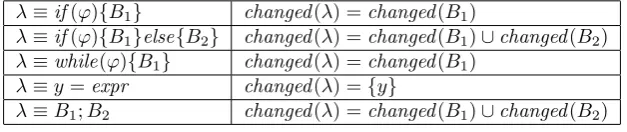
Based on the definition of variables in an expression we define which variables areused orchanged by a statementλ,used(λ) orchanged(λ), in table 4.2.

λ≡if(ϕ){B1} used(λ) =vars(ϕ)∪used(B1)

λ≡if(ϕ){B1}else{B2} used(λ) =vars(ϕ)∪used(B1)∪used(B2)

λ≡while(ϕ){B1} used(λ) =vars(ϕ)∪used(B1)

λ≡y=expr used(λ) =vars(expr)

[image:35.595.123.437.351.417.2]

λ≡B1;B2 used(λ) =used(B1)∪used(B2)

Table 4.1: The functionused

λ≡if(ϕ){B1} changed(λ) =changed(B1)

λ≡if(ϕ){B1}else{B2} changed(λ) =changed(B1)∪changed(B2) λ≡while(ϕ){B1} changed(λ) =changed(B1)

λ≡y=expr changed(λ) ={y}

λ≡B1;B2 changed(λ) =changed(B1)∪changed(B2)

Table 4.2: The functionchanged

We define a special kind ofused,directly used, to indicate that a variable is used

in a guard, synchronization or an invariant.

• On an edge:

– aisdirectly used in the guard of an edgeeifa∈used(guard(e)). – a is directly used in the synchronisation part of an edge if a ∈

vars(channel(e)).

– The set of all directly used variables of an edge eisdir used(e)

• At a location:

– aisdirectly used at a locationl ifa∈used(I(l)).

– The set of all directly used variables of l isdir used(l)

A problem with the linear process equations of [30] was that, by linearising the original processes into one linear form, the original control flow was lost. This control flow needed to be reconstructed first, therefore they included

def-initions of source and destination functions as well as a definition called rules

to determine if a parameter is a control flow parameter or a data parameter.

(36)

whereas the other variables are the Data Variables (DPs), which can be divided into local and global variables.

Definition 6 (Local & Global variables). We have a network P of timed

automata Pi. Let a ∈ VP ∪CP be a variable, which is alocal variable of Pi

if all edges that change or use a are part of the set of edgesEPi. A variable

that is not a local variable of one of the timed automata inP is a global variable.

• ais local in Pi ifa ∈used(Pi)∨a∈ changed(Pi)∧ ∀j·i 6=j =⇒ a /∈

used(Pj)∧a /∈changed(Pj)

• ais global in P if∀Pi∈P·a /∈local(Pi)

From this point we use the set A for referring to all variables, data or clock,

(37)

4.2

Relevance algorithm

The next step is the relevance algorithm itself. This algorithm will identify if a variable is relevant at a given location or not. If a variable is not relevant at a particular point it can be reset to its initial valuation. We first present a basic version of the algorithm and

Definition 7 (Relevance). For a network P of simple timed automata Pi,

1 ≤i ≤n, with n the number of automata, variables a, b∈ A and a location

l∈LPi. We use (a, l)∈R (orR(a, l)) to denote that the value ofais relevant

at locationl. FormallyRis the smallest relation such that:

1. If ais directly used in somee∈EP, a∈dir used(e) and l=src(e) then

RP(a, l)

2. If ais directly used at some location l,a∈dir used(l) thenRP(a, l)

3. If ais used in a property then: ∀l∈LP·RP(a, l)

4. If RP(b, l0), ∃e ∈ EP such that src(e) = l and target(e) = l0, such that

a∈processSeq(Λ(update(e)),{b}) thenRP(a, l)

5. If RP(b, l0), ∃e ∈ EP such that src(e) = l, l ∈ LPi, l

0 _∈ _L

Pj and i 6= j,

such thata∈processSeq(Λ(update(e)),{b}) thenRP(a, l)

Explanation of the algorithm For a better understanding we briefly de-scribe each of the five clauses:

1. A variable is directly used on an edge if it is either used in a guard or in the synchronisation part of an edge. If that is the case this variable directly influences the control flow of the program and needs to be marked relevant at the source of the edge.

2. The same holds for a variable that is used in an invariant of a location. Because an invariant needs to be true at a location the values of the variables used in that invariant are also important making it necessary for the variables to be marked relevant.

3. A variable that is used in a property is automatically marked relevant at

all locations ofP. Because a change in the value of such a variable could

cause a change in the truth value of the property therefore the values of these variables are relevant. (see section 4.3.3 for an improvement on this)

4. This clause takes care that if a variable is relevant at the target location of an edge that than every variable that is used in the rhs of an assignment to this relevant variable is also marked relevant. If there is no assignment then the relevant variable itself also becomes relevant at the source location as its value is already important at that point. Finally we mark variables relevant that are used in conditional statements (for instance the condition of an if-statement).

5. The last clause takes care of the same as the 4th_{clause but not for variables}

(38)

Algorithm 1processSeq(stmt seq statements, variable relevant)

1: if (statements.isEmpty())then

2: return relevant

3: else

4: relevant = processStat(statements.tail() , relevant)

5: return processSeq(statements.withoutTail() , relevant)

6: end if

Algorithm 2processStat(single stmt stat , sethvariablesirelevant)

1: if (stat≡u = expr)then

2: if (u∈relevant)then

3: removeVar(u, relevant)

4: for allvar∈used(expr) do

5: insertVar(var, relevant)

6: end for

7: end if

8: else if (stat≡if(ϕ)B1 elseB2)then

9: for allvar∈vars(ϕ)do

11: end for

12: relevant = relevant∪processSeq(B1), relevant)

13: relevant = relevant∪processSeq(B2), relevant)

14: else if (stat≡while(ϕ)B)then

15: while(relevant6= temp)do

16: temp = relevant

17: for allvar∈vars(condition)do

19: end for

20: relevant = relevant∪processSeq(B, relevant)

21: end while

22: end if

23: return relevant

Algorithm 3insertVar(variable var, sethvariablesirelevant)

1: relevant.insert(var)

(39)

Algorithm 4removeVar(variable var, sethvariablesirelevant)

1: relevant.remove(var)

Why do we need a While-loop in line 14? The necessity of the while-loop can be explained by the following UPPAAL code fragment:

1 . . .

2 w h i l e( . . . ) do

3 a=b ;

4 b=c ;

5 end w h i l e

6 . . .

7 }

Listing 4.9: Example demonstrating the ne

Reducing UPPAAL models through control flow analysis

REDUCING UPPAAL

Contents

CHAPTER 1

Initial exploration

Research Questions

UPPAAL?

CHAPTER 2

OF F ON DIM

Reduction techniques

Slicing

Partial order reduction

Dead variable analysis

Exact (clock) acceleration

Active clock reduction

Compiler optimisation techniques

Dead Code Elimination

Code Motion

Constant Propagation

Global Value Numbering and redundant

Basic timed automata

Clocks

Channels

Semantics

Parallel composition

The Extended Timed Automata Formalism

Syntax of the Imperative Language

Syntax of Extended Timed Automata

Semantics of the imperative language

CHAPTER 4

Rewriting of the update statements

Changed, used and directly used

Relevance algorithm