Analysis of Hydrostatic Tube Bulging with Cylindrical Die Using Static Explicit FEM*

Analysis of Hydrostatic Tube Bulging with Cylindrical Die Using

Static Explicit FEM

Takayuki Hama

_{, Motoo Asakawa}

_{, Sadakatsu Fuchizawa}

_{and Akitake Makinouchi}

Department of Mechanical Engineering, Waseda University, Tokyo 169-8555, Japan

2_{Integrated Volume-CAD System Program, The Institute of Physical and Chemical Research-RIKEN, Saitama 351-0198, Japan} 3_{Department of Mechanical Systems Engineering, Utsunomiya University, Utsunomiya 321-8585, Japan}

Tube Hydroforming (THF) is getting an increasing amount of attention in industry. THF has advantages such as weight reduction, high dimensional accuracy, and high rigidity. However, this forming process requires precise control of internal pressure and axial feeding. Additionally, in most cases prebending processes must be performed on the tubes before the hydroforming process can be carried out, and the forming ability of the hydroforming processes is influenced by the outcome of this prebending process. We describe the development of the Finite Element Method (FEM) code for THF analysis and a comparison of experimental and analytical results. The elastoplastic FEM code for THF analysis has been developed based on ITAS3D which is a sheet-metal-forming simulation program using the static explicit method. The algorithm of hydraulic pressure has been newly implemented in ITAS3D. Hydrostatic copper tube bulging with a cylindrical die was calculated with the code, and analytical results show good agreement with experimental ones. In this calculation, there is only a very small difference between the solid element and shell element results.

(Received July 18, 2002; Accepted January 21, 2003)

Keywords: tube hydroforming, elastoplastic finite element method, static explicit method, discretization of hydraulic pressure, strategy of discontact

1. Introduction

Recently, from the viewpoint of the preservation of the global environment and impact-damage resistance, product design which satisfies both lightweight structure and high rigidity simultaneously has become a task which requires special techniques in the automobile industry. Tube hydro-forming is one technology that can be used to achieve both targets, as well as to save costs. Recently, this technology has been gaining increasing attention in industry.

Tube hydroforming caters to the demands of weight reduction as it requires, for example, fewer parts, higher dimensional accuracy, and higher rigidity compared to conventional manufacturing methods. Applications of tube hydroforming can now be found in the automobile and aircraft industries.1–4)

There still are, however, difficult problems to which conventional technical know-how cannot be applied, such as control of hydraulic internal pressure and the amount of feeding in the longitudinal direction. The capability of the hydroforming process is also largely governed by the outcome of the prebending processes. As a result, various types of defects, such as buckling and breakage, may occur if the process parameters are not properly set. These parameters normally are determined by trial and error.

Fundamental aspects of the tube hydroforming process have been studied experimentally and theoretically.1,5–11) Through these studies, process characteristics of tube hydro-forming have been gradually understood. On the other hand, there are few reports on the formability of actual engineering parts, from either an experimental or theoretical point of view.12,13)Although in some studies the tube bending process

has been considered as a preforming process of tube hydroforming,14) studies on multistage processes are scarce.15)

In this paper, we describe the development of the finite-element-method (FEM) code for the simulation of the tube hydroforming process. The elastoplastic FEM code has been developed based on ITAS3D16) which is a sheet-metal-forming simulation program using the static explicit method. The simulation of hydrostatic tube bulging with a cylindrical die was carried out and a comparison of experimental and analytical results was performed to verify the validity of the code.

2. Finite-Element Formulation

2.1 Variational principle

ITAS3D is a sheet-metal-forming-simulation program based on elastoplastic FEM using the static explicit method. The updated Lagrangian rate formulation is used to describe the finite deformation. The rate form of the equilibrium equations and boundary conditions are equivalently expres-sed by the principle of virtual work in the rate form:17)

Z

V

fðJ_ij2ikDkjÞDijþjkLikLijgdV

¼

Z

S

_

F

F

F

FividSþ

Z

SC _

f

f

f

f_ividS;

ð1Þ

whereVandSdenote, respectively, the domain occupied by the body and its boundary at time t. S is the part of the boundary S on which the rate of hydraulic pressure FF_ is prescribed.SCis the part of the boundarySon which the rate

of tractionff_(other than the hydraulic pressure) is prescribed. Hence, the boundarySt on which the total rate of traction is

prescribed is given as St¼SCþS. is the Cauchy stress tensor;J_{is the Jaumann rate of the Kirchhoff stress tensor;}

*1_{This Paper was Originally Published in Japanese in the Journal of JSTP,}

43, (2002) 1.

*2_{Graduate Student, Waseda University.}

L is the velocity gradient tensor; and D is the strain rate tensor, which is the symmetric part of L. v is the virtual velocity field satisfying the conditionv¼0on the velocity boundary. The only difference between eq. (1) and the one proposed by McMeeking and Rice17)is the assumption that the volume of the body does not change, i.e., detðFÞ ¼ detðx=XÞ ¼1. As a result of this assumption, J_¼J _is

achieved.

2.2 Constitutive equation

Small-strain linear elasticity and large deformation, rate-independent work-hardening plasticity is assumed. Hill’s quadratic yield function18)and the associated flow rule are used. The elastoplastic constitutive equation can be written in the form

J_ij¼Cep_ijklDkl¼C ep

ijklLkl; ð2Þ

whereC_ijklep is the tangent elastoplastic modulus.

Introducing eq. (2) into eq. (1), the final form of the principle of virtual work is obtained as

Z

V

DijklLklLijdV¼

Z

S

_

F

F

F

FividSþ

Z

SC _

f

f

f

fividS; ð3Þ

where Dijkl¼Cijklep þijkl and ijkl¼1₂ðjlikikjl

iljkjkilÞ.

2.3 Finite-element equations

The procedure for solving the formulation stated above follows the standard process of static explicit analysis. Equations (2) and (3) are integrated from time t totþt, where t is a small time increment. The displacement increment, the Jaumann stress increment and the increment of the displacement gradient are written as

u¼vt; J¼Jt; L¼Lt;

and all the rate quantities are simply replaced by incremental quantities, assuming that rates are kept constant within an increment. Performing a standard finite-element discretiza-tion, eq. (3) can be replaced by a system of algebraic equations:

Ku¼FþFCþCC; ð4Þ

whereKis the elastoplastic stiffness matrix. The termsFC,

F and CC come from the right-hand side of eq. (3)

where the derivative ff_ must be replaced by the expression

_

ff ¼ff_ieiþff_jej (sum on i and j). The term FCfiei

denotes the increment of the external force vector and the termCCfiei expresses the rotation of the total force

vector during the increment. The replacement of the derivative FF_ by the expression stated above will be shown in the next section.

In the ITAS3D code, a static-explicit approach to a solution of eq. (4) is applied. The stiffness matrix K is described at time t, and is considered constant within the incrementt. The generalizedrminmethod19)is employed to limit the size of the increments.

2.4 Formulation of hydraulic pressure

A discretization of the hydraulic pressure is shown.20–22)A degenerated 4-node shell element and an 8-node solid

element are employed in the simulation, so that the discretization for these elements is performed.

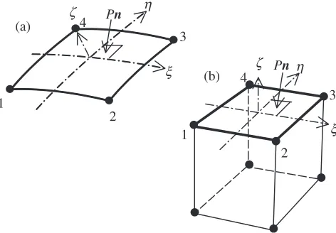
Let us consider a rectangular element on which the hydraulic pressure vectorPnacts.Pnis assumed to act upon the middle surface of shell elements and upon an element surface of solid elements, as illustrated in Fig.1. Assuming the hydraulic pressure vector to be traction, the equivalent nodal force increment vectorFefor an element of the form

Fin eq. (4) is given as Fe¼

Z

Se

TðPnÞdS

¼ P

Z

Se

T_ndS

eP

Z

Se

T_ndS

e;

ð5Þ

where Se denotes the element area on which the hydraulic

pressure acts, is a [312] matrix consisting of shape function Nk_{, and n is the unit normal. and n are}

respectively given as

¼

N1 0 0 N4 _{0 0}

0 N1 0 0 N4 0

0 0 N1 _{0 0 N}4

2 6 4

3 7

5; ð6Þ

n¼

@x

@

@x @ @x

@

@x

@

: ð7Þ

The first term of the right-hand side of eq. (5) denotes a vector of the hydraulic pressure increment and the second term expresses the rotation of a vector of the total hydraulic pressure during the increment. The following relations can be employed on the surfaceSe:

x¼Nkxk_{; ðk¼1;. . .;4Þ ð8Þ}

dSe¼

@x

@

@x

@

dd; ð9Þ

where xk _{denotes the coordinates of the element nodes.}

Introducing eqs. (8) and (9) into the first term of the right-hand side of eq. (5), the vector of the hydraulic pressure increment is obtained as

(a)

(b) ξ

η

ζ Pn

1

2

3 4

ξ η ζ Pn

1

2

3 4

P

Z

Se

TndSe

¼P

Z1

1

Z1

1

T @N

k @ x k @N l @ x l

dd:

ð10Þ

The incremental form ofn(eq. (7)) can be written as

n¼ @Nk

@ x

k @N l @x l

þ @N

m @ x m @N n

@x

n @x @ @x @

: ð11Þ

Introducing a vector of the element nodal point displacements increment,

ue fx11;x 1 2;x

1 3;x

2

1; ;x 4 2;x

4 3;g

T_{; ð12Þ}

where the subscriptjonxi_j denotes the directionX,Y, orZ, and the superscriptionxi_jdenotes the node number, into eq. (11), we obtain

n¼ 1

@x @ @x @

e1jk

@xj

@ @Nl

@

@xj

@ @Nl

@

xl_k

e2jk

@xj

@ @Nl

@

@xj

@ @Nl

@

xl k

e3jk

@xj

@ @Nl

@

@xj

@ @Nl

@

xl_k

8 > > > > > > > > < > > > > > > > > : 9 > > > > > > > > = > > > > > > > > ;

Mue

@x @ @x @

; ð13Þ

where eijk is the permutation symbol, j;k¼1;2;3, and

l¼1;. . .;4.Mis a [312] matrix. Introducing eq. (13) into the second term of the right-hand side of eq. (5), the rotation of a vector of the total hydraulic pressure is obtained in the form

P

Z

Se

TndSe¼ P

Z1

1

Z1

1

TMddue: ð14Þ

Equation (14) can be rearranged as P

Z1

1

Z1

1

TMddueKenue; ð15Þ

whereKe_nis a [1212] matrix. According to the boundary conditions applied to the edge of the tube, in some casesKe_n

becomes asymmetric.

By using eqs. (5), (10) and (15), the element stiffness equation is finally obtained as

Fe¼ P

Z1

1

Z 1

1

T @N

k @ x k @N 1 @ x l

ddKe_nue:

ð16Þ

Introducing eq. (16) into the element form of eq. (4) and moving the second term of the right-hand side of eq. (16) to the left-hand side of the equation, we get the final form of the element stiffness equation:

ðKeþKenÞue¼ P

Z1

1

Z1

1

T @N

k @ x k @N l @ x l

ddþFe

cþC e c:

ð17Þ

By assembling eq. (17), we ultimately obtain the global stiffness equation for the hydroforming simulation.

2.5 Strategy of discontact for shell elements

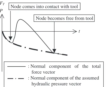
In the sheet stamping simulation, if the normal component of the total force vector becomes 0, the contact node is considered to become free from tool.23) However, it is impossible to separately define the nodes on which the tool reaction force vector acts and on which the hydraulic pressure vector acts in the hydroforming simulation using shell elements, because there is only one node in the thickness direction. As a result, the conventional strategy of discontact used in ITAS3D is not applicable in the hydroforming simulation using shell elements. Hence, a new strategy of discontact is proposed.

In ITAS3D, the total force vector associated with the contact node represents the tool reaction force vector. In this strategy, the assumed hydraulic pressure vector which may actually act on the contact node is calculated separately. When the normal component of the total force vector becomes equivalent to that of the assumed hydraulic pressure vector, that is,Pin eq. (5), then the contact node is considered to become free from tool. This strategy is schematically shown in Fig.2. In this figure, the normal component of the total force vector is set to be positive and that of the assumed hydraulic pressure vector is set to be negative. Based on the above,rmin with respect to discontact can be written in the form

rmin ¼

PFT

FTP

; ð18Þ

whereFT denotes the normal component of the total force

vector, FT is the increment of FT, P is the normal

3. Simulation of Tube Bulging with Cylindrical Die

3.1 Analytical model

A copper tube subjected to hydrostatic bulge forming with a closed die6)is calculated to verify the validity of the code developed in this study.

Figure3 shows the geometries of the cylindrical die and the bulged tube used in the simulation. Considering the symmetric property of the deformation, the tube is divided into 4 parts in the circumferential direction, and 2 parts in the longitudinal direction and thus a 1/8 part is modeled. The symmetrical boundary conditions are applied to the nodes on the symmetry planes. The edges of the tube are aligned with the longitudinally rounded part of the die and the nodes on the edges are fixed in the longitudinal direction. The Coulomb friction law is assumed for friction between the die and the tube, and a coefficient of friction of 0.1 is assigned. However, the tube does not slide on the tool surface in this deformation process, so the influence of friction would be negligible.

An annealed seamless deoxidized copper tube is used as the blank. The dimensions are 40 mm outer diameter, 80 mm length and 1 mm wall thickness. Swift equation is used to

model the stress-strain curve. Mechanical properties of the tube adopted in the simulation are shown in Table1.

Four-node degenerated shell elements and 8-node solid elements are employed for the tube model. Assumed strain field (ASF) elements24) and selective reduced integration (SRI) elements are respectively used for shell elements and solid elements. For the tube meshes, 10 divisions in the circumferential direction and 40 divisions in the longitudinal direction are made, as well as 2 divisions in the thickness direction for solid elements.

This forming process can be divided into two stages: the free bulging process and the deformation process after coming into contact with the die. In this study, the radial expansion at the center of the tuberc(within the range of

0:0 mmrc6:0 mm) for the free bulging process and the contact length between the tube and the straight part of the die Ld for the deformation process after coming into contact with the die are taken as the parameters to represent each deformation process. The definitions of these para-meters are shown in Fig.3.

3.2 Comparison of analytical and experimental results The relationship between the hydraulic internal pressure and the radial expansion at the center of the tube within the free bulging process is shown in Fig.4. We can see that the radial expansionrcgradually increases up to 8 MPa, after which it increases exponentially. There is good agreement between the simulated and experimental results. Although some difference between the result obtained with solid elements and that obtained with shell elements is seen and the former is closer to the experimental result than the latter, this difference is negligible and it can be said that both results are in good agreement with that of the experiment.

Subsequently, the tube begins to come into contact with

Fig. 3 Geometry of the die and the bulged tube.rc: radial expansion, L: distance from the center of the tube,Ld: Contact length between the tube and the straight part of the die.

Table 1 Mechanical properties adopted in the simulation.

E

y Fvalue n "0

r

/GPa /MPa /MPa value value

125 0.3 60 481 0.38 0.016 1.0

_{The true stress-logarithmic plastic strain curve is approximated by}

¼Fð"0þ"PÞn. E: Young’s modulus, : Poisson’s ratio, y: Yield

stress. FT

P

t

Node comes into contact with tool

Node becomes free from tool

: Normal component of the total force vector

: Normal component of the assumed hydraulic pressure vector

Fig. 2 The strategy of discontact for hydroforming simulation using shell elements.

0 1 2 3 4 5 6

0 2 4 6 8 10 12

Radial expansion,

∆

rc

/mm

Shell element

Solid element : Experiment

Internal pressure, P/MPa

the straight part of the die. The relationship between the hydraulic internal pressure and the contact length between the tube and the straight part of the die is shown in Fig. 5. Initially, the contact length increases exponentially, just like the increase of the radial expansion in the range of internal pressure of 8 to 10 MPa, as shown in Fig.4. It finally saturates at 30 MPa. This result also shows good agreement between the simulated and experimental results.

Figures4 and 5 show that the relationship between the hydraulic internal pressure and the deformation process,i.e., the tube expands exponentially from 8 to 30 MPa, is well reproduced in the simulation.

The distributions of circumferential strain in the long-itudinal direction at several stages obtained from the simulation with shell elements and that with solid elements are compared with those from the experiment in Fig. 6. In

this figure, the origin of the horizontal axis corresponds to the center of the tube, and the stages atrc¼3:6, 4.4, 5.4 mm andLd¼18:2mm are shown. Good agreements can be seen between the experimental results and analytical ones with both solid elements and shell elements. It can be considered that the circumferential strain distribution represents the profile of the deformed tube, so we can say that Fig.6shows good agreement in the profiles of the deformed tube at each stage of the deformation process.

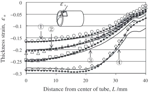
The distributions of thickness strain in the longitudinal direction at several stages, obtained from the simulation with shell elements and that with solid elements, are compared with those from the experiment in Fig. 7. The definition of calculated thickness strain is unclear when solid elements are used, because the nodes which were aligned in the thickness direction before the deformation are not in line after the deformation. Therefore, in this study, we define the thickness strain of the tube in the simulation using solid elements as the average between the calculated thickness strain on the nodes on the outer surface and that on the inner surface, as shown in Fig.8.

The stages shown in Fig.7are the same as those in Fig. 6. Although small differences are seen near the edge of the tube and the calculated thickness strain near the edge is larger than

0 5 10 15 20 25 30

0 10 20 30 40 50

Shell element Solid element

Internal pressure, P /MPa

Contact length,

Ld

/mm

: Experiment

Fig. 5 Relationship between the internal pressure and the contact length.

0 0.05

0.1 0.15 0.2 0.25 0.3

0 10 20 30 40

Distance from center of tube, L /mm

Circumferential strain,

εθ

εθ

Exp. Deformed condition Shell

Solid Shell Solid Shell Solid Shell Solid Calculation

Ld=18.2mm

∆rc=3.6mm

4.4

5.4 Notations for

Figs. 6, 7

Fig. 6 Distribution of circumferential strain in the longitudinal direction at several stages.

−0.3 −0.25 −0.2 −0.15 −0.1 −0.05 0

0 10 20 30 40

Thickness strain,

εn

Distance from center of tube, L /mm εn

Fig. 7 Distribution of thickness strain in the longitudinal direction at several stages.

Fig. 8 Definition of thickness strain in the case of using solid elements. l_{: Thickness strain at the node on the outer surface.}s_{: Thickness strain at} the node on the inner surface."n: Average ofsandl, which is taken to be

that in the experiment in all cases, we can see good agreement between the experimental results and the analy-tical ones for both shell elements and solid elements. The reason for the difference near the edge is considered to be the difference in the way of fixing the edge between the experimental model and the analytical model. However, the development of thickness strain near the edge can also be seen in the experimental result, so we can say that qualitative agreement is achieved.

On the basis of the results presented above, it can be said that the calculated strain distributions show good agreement with the experimental ones, as well as the relationship between the hydraulic pressure and the deformation process. Hence, these results confirm the high accuracy of the code developed in this study. Moreover, they also clarify that the results obtained with shell elements are sufficiently accurate compared to those obtained with solid elements in the calculation of thin tube hydroforming.

4. Conclusions

An elastoplastic FEM code for the simulation of the tube hydroforming process was developed based on the static explicit code ITAS3D. The formulation of the hydraulic pressure boundary condition and a new strategy of discontact for shell elements were newly implemented in ITAS3D. The simulation of hydrostatic tube bulging with a cylindrical die was performed. Results obtained in this study are summar-ized as follows.

(1) Good agreements were seen between the simulated and experimental results in terms of not only the relation-ship between the hydraulic pressure and the deforma-tion process but also strain distribudeforma-tions. This confirmed the validity of the code.

(2) It was clarified that the results obtained with shell elements are sufficiently accurate compared to those obtained with solid elements in the calculation of thin tube hydroforming.

REFERENCES

1) F. Dohmann and Ch. Hartl: J. Mater. Process. Technol.71(1997) 174– 186.

2) J. Shao and Y. Shimizu: Proc. Int. Seminar on ‘‘Recent status & trend of tube hydroforming’’, (The Japan Society for Technology of Plasticity, 1999) pp. 73–79.

3) M. Ahmetoglu, K. Sutter, X. J. Li and T. Altan: J. Mater. Process. Technol.98(2000) 224–231.

4) M. Ahmetoglu and T. Altan: J. Mater. Process. Technol.98(2000) 25– 33.

5) M. Koc and T. Altan: J. Mater. Process. Technol.108(2001) 384–393. 6) S. Fuchizawa: Proc. 3rd Int. Conf. Technology of Plasticity (Kyoto

1990) pp. 1543–1548.

7) S. Fuchizawa, M. Narazaki and A. Shirayori: Proc. 5th Int. Conf. Technology of Plasticity, ed. by T. Altan, (Ohio 1996) pp. 497–500. 8) B. J. MacDonald and M. S. J. Hashmi: J. Mater. Process. Technol.103

(2000) 333–342.

9) M. Koc, T. Allen, S. Jiratheranat and T. Altan: Int. J. Mach. Tools Manuf. Des. Appl.40(2000) 2249–2266.

10) B. Carleer, G. van der Kevie, L. de Winter and B. van Veldhuizen: J. Mater. Process. Technol.104(2000) 158–166.

11) K.-i. Manabe and M. Amino: J. Mater. Process. Technol.123(2002) 285–291.

12) L. P. Lei, J. Kim and B. S. Kang: Int. J. Mach. Tools Manuf. Des. Appl.

40(2000) 1691–1708.

13) A. Kellicut, B. Cowell, K. Kavikondala, T. Dutton, S. Iregbu and R. Sturt: Proc. 4th Int. Conf. on Numerical Simulation of 3D Sheet Forming Processes (NUMISHEET’99), ed. by J. C. Gelin and P. Picart, (BURS, Besancon 1999) pp. 509–514.

14) K. Manabe and S. Nakamura: Proc. 4th Int. Conf. on Numerical Simulation of 3D Sheet Forming Processes (NUMISHEET’99), ed. by J. C. Gelin and P. Picart, (BURS, Besancon 1999) pp. 503–508. 15) J. Yang, B. Jeon and S. I. Oh: J. Mater. Process. Technol.111(2001)

175–181.

16) M. Kawka and A. Makinouchi: J. Mater. Process. Technol.50(1995) 105–115.

17) R. M. McMeeking and J. R. Rice: Int. J. Solids Struct.11(1975) 601– 616.

18) R. Hill: Proc. R. Soc.193A(1948) 281.

19) Y. Yamada, N. Yoshimura and T. Sakurai: Int. J. Mech. Sci.10(1968) 343–354.

20) Z. G. Sun and A. Makinouchi: Collected abstracts of the 12th computational mechanics conference (Japan society of Mechanical Engineers, 1999) pp. 703–704 (in Japanese).

21) H. L. Xing and A. Makinouchi: Int. J. Mech. Sci.43(2001) 1009–1026. 22) W. K. Liu, E. S. Law, D. Lam and T. Belytcshko: Comput. Methods

Appl. Mech. Eng.55(1986) 259–300.

23) M. Kawka and A. Makinouchi:Huber’s Yield Criterion in Plasticity, (AGH, Krakow, 1994) pp. 241–266.