Evaluating the Accuracy of Valuation Multiples on Indian Firms Using Regularization Techniques of Penalized Regression

(1)

ISSN Online: 2162-2086 ISSN Print: 2162-2078

DOI: 10.4236/tel.2019.91015 Feb. 3, 2019 180 Theoretical Economics Letters

Evaluating the Accuracy of Valuation Multiples

on Indian Firms Using Regularization

Techniques of Penalized Regression

Vandana Gupta

Institute of Management Technology, Ghaziabad, India

Abstract

This research study is conducted on companies in three prominent sectors: Automobile, Banking and Steel—all three diverse and affected by different economic, fiscal and financial policies. The author Gupta [1] attempts to ex-tend the scope of study done earlier using simple linear regression for valua-tion of companies. Highlighting the limitavalua-tions of linear regression: multicol-linearity and normality, the present study is conducted by applying regulari-zation techniques of machine learning. Ridge regression, LASSO and elastic net techniques are employed to underscore this commonality of the set of valuation multiples. These regularization techniques are tested on data of In-dian listed firms spanning across twelve years from FY 07 to FY 2018 and the four multiples identified for the study are 1) price to earnings (P/E), 2) price to sales (P/S), 3) enterprise value to earnings before interest tax depreciation and amortization (EV/EBIDTA) and 4) price to book value (P/BV). The em-pirical findings are based on root mean square errors and learning curves, which corroborate the least prediction errors in P/S for auto sector, EV/EBIDTA for steel sector and P/BV for banking sector. As a byproduct, the author has also been able to pinpoint which one of the variables among them is the most important. The study concludes that, in spite of differing sectors, a certain set of common variables can be used across them to effectively assess company valuation (valuation multiples). The present work contributes to emerging market literature by evaluating the key multiples that drive sectors to apply non-traditional regression techniques.

Keywords

Valuations, Prediction, Earnings, Book Value, Enterprise Value, Ridge, Lasso, Elastic Net

How to cite this paper: Gupta, V. (2019) Evaluating the Accuracy of Valuation Mul-tiples on Indian Firms Using Regulariza-tion Techniques of Penalized Regression. Theoretical Economics Letters, 9, 180-209. https://doi.org/10.4236/tel.2019.91015

Received: October 19, 2018 Accepted: January 31, 2019 Published: February 3, 2019

(2)

DOI: 10.4236/tel.2019.91015 181 Theoretical Economics Letters

1. Introduction

1.1. Business Valuations

Business valuation is the process of determining the economic value of a busi-ness or company. Busibusi-ness valuation can be used for a variety of reasons, in-cluding sale value, establishing partner ownership, and assessing property among others. Often, owners will turn to professional business valuators for an objective estimate of the business value.

No one business valuation approach or method is definitive. Hence, it is common practice to use a number of business valuation methods under each approach. The business value then is determined by reconciling the results ob-tained from the selected methods. Typically, a weight is assigned to the result of each business valuation method. Finally, the sum of the weighted results is used to determine the value of the subject business.

This process of concluding the business value is referred to as the business value synthesis.

1.2. Business Valuation Approaches and Methods

There are three fundamental ways to measure the value of a business (Jenkins [2]): Asset Approach: The asset approach to business valuation considers the un-derlying business assets in order to estimate the value of the overall business en-terprise. This approach relies upon the economic principle of substitution and seeks to estimate the costs of recreating a business of equal economic utility, i.e.

a business that can produce the same returns for its owners as the subject busi-ness.

The business valuation methods under the Asset Approach include:

 _{Asset accumulation method.}  Capitalized excess earnings method.

Market Approach: Under the Market Approach to business valuation, one consults the market place for indications of business value. Most commonly, sales of similar businesses are studied to collect comparative evidence that can be used to estimate the value of the subject business. This approach uses the eco-nomic principle of competition, which seeks to estimate the value of a business in comparison to similar businesses whose value has been recently established by the market.

The business valuation methods under the Market Approach are:

 _{Comparative private company transaction method.}  Comparative publicly traded company transaction method.

Income Approach: The Income Approach to business valuation uses the eco-nomic principle of expectation to determine the value of a business. To do so, one estimates the future returns the business owners can expect to receive from the subject business. These returns are then matched against the risk associated with receiving them fully and on time.

(3)

ex-DOI: 10.4236/tel.2019.91015 182 Theoretical Economics Letters

pected to be received by the business owners in the future. The risk is then quan-tified by means of the so-called capitalization or discount rates.

The methods which rely upon a single measure of business earnings are re-ferred to as direct capitalization methods. Those methods that utilize a stream of income are known as the discounting methods. The discounting methods ac-count for the time value of money directly and determine the value of the busi-ness enterprise as the present value of the projected income stream.

The methods under the Income Approach include:

 Discounted cash flow method.

 Multiple of discretionary earnings method.

 Capitalization of earnings method.

Concept of Relative Valuation: Market based valuation use the comparable companies approach or relative valuation techniques to value the equity or en-terprise based on average multiple of the peer group and a value driver.

Relative valuation is a significant aspect in the intrinsic value analysis of a company and could possibly be considered as one of the early forms of valuation in the simplest linear form by comparing the basic performance of one company relative to another company. The concept of relative valuation presents a com-parative cohesive study of companies that would be structured on pivotal ele-ments that establishes the basis for a collective study. These pivotal eleele-ments would be represented by key value drivers as the dependable variables being a function a series of independent variables that would all be comparable. Howev-er, the initial process should focus on specifying the key value drivers that would outline the foundation for relative valuation, such as considering multiples.

Multiples are considered as being a function of the future performance of a company in terms of its share price, and some of the commonly applied mul-tiples in a share valuation are the Price-to-Earnings (PE) ratio, Price to Book Value (PBV) and Price to Sales (PS). Another multiple that is significant for val-uations is the Enterprise Value to Earnings before Interest, Tax, Depreciation and Amortization (EV/EBIDTA). Relative valuation could essentially be per-ceived as a comparative analysis structuring a systematic method in estimating the share price of a company that would be significantly reliable. Thus, the me-chanisms of a relative valuation process would analyze and compute an intrinsic value that should be clearly defined, especially as the computation result would be synthesized from a selection of comparative variables that are relative to companies and the market as a whole. Consistency would be maintained by as-sessing the same list of variables for all the companies represented in the sample being analyzed.

1.3. Multiples and Their Interpretation

(4)

compared to peers means it can turn around and its shares will enjoy substantial increase with the increase in its P/Sales ratio. For a small company or a start-up where there is a negative number to show for earnings, a P/S ratio can come in handy to calculate the intrinsic value.

EV/EBITDA Ratio is also known as the ‘Enterprise Multiple’. It is used as a valuation tool to compare the value of a company, debt included, to the compa-ny’s cash earnings less non-cash expenses and remains unaffected by changing capital structures and thus offers fairer comparisons.

EV/EBITDA value below 10 is commonly interpreted as healthy and above average.

Price/Book Value is known as Price/Book value ratio. It can be interpreted as the ratio of (Stock price x No. of outstanding shares) and sum of the book values of Equity of the company. It is a good metrics to value stocks of companies in the financial services sectors. Generally, a low P/BV ratio means that the market believes the assets of the company are undervalued and are expected to earn high returns on its assets. The price to book value (P/BV) measures how much are the markets are willing to pay for the measured accounting value of a company’s as-sets.

Price/Earnings Ratio is the ratio of price of stock and EPS. It can be inter-preted as ratio of Market Value of the company and the EPS. It indicates the amount an investor can expect to invest in the company in order to receive one rupee of that company’s earnings. Generally, a high P/E ratio means that inves-tors are anticipating higher growth in the future. While it is amongst the easiest valuation multiple to calculate and compare, the P/E is highly prone to manipu-lation because it is based on the “earnings” number that is an easy candidate for manipulation by companies and their accountants.

While for both developed and emerging economies valuation is of immense significance since investor decisions vest on this tenet. Therefore, there is in-creasing emphasis on methodologies to value companies and their stock. With the globalization of world economy and subsequent mobilization of funds in the form of joint ventures, M&As, and other strategies of corporates, it is imperative that valuations be done based on appropriate methodologies.

1.4. Objectives of the Study

The present study chooses to evaluate the predictive ability of four multiples across three sectors. The broad objectives are:

• _{To apply ridge regression, LASSO and Elastic Net techniques to valuation}

multiples.

• To identify the multiple with least prediction error using Root Mean Square Error (RMSE) and learning curves for each sector.

• _{To find the predictors which best explain the valuation multiples for each}

sector.

(5)

To present the study in a more lucid manner the paper is organized as follows. Section I is on Introduction while Section II reviews related literature. Section III presents the research design and methodology while the empirical findings are presented in Section IV. Section V gives the conclusion coupled with scope for future research.

2. Review of Literature

The research in this field can be classified into two: those based on comparable company’s approach and those based on fundamental drivers.

Bulk of prior research is focused on either on how comparable firms should be identified for the simple multiple valuation or which valuation multiple is supe-rior in terms of the valuation accuracy. Considerable research has also been done on identifying not a standalone multiple but a combination of multiples which best reflect the value of stock of a firm. The pioneer of this theory was Alford [3]

who used a combination of factors to select the best combination of comparable firms. Among the factors chosen were combinations of industry type, growth (ROE) and size. He affirmed that valuation errors are minimized when the right choice of comparable firms is made. Penman [4] estimated the weights required to use combined earnings and book value multiples for valuing equity. Liu et al. [5] advocated that multiples derived from value drivers based on forward earn-ings explain the stock prices best. Yoo [6] advocated that combining several simple multiple valuation outcomes of a firm, each of which is based on a stock price multiple to a historical accounting performance measure of the compara-ble firms (historical multiple), improves the valuation accuracy of the simple multiple valuation using a single historical multiple. Antonios et al.[7] explored the sensitivities of three multiples P/E, P/BV and P/Sales in terms of their biases and concluded that for most definition of comparable firms, the P/S valuation method performs better when considering mean and P/BV performs well when evaluating on the basis of median.

Some of the other research works include by Nel et al.[8] established that eq-uity-based multiples are superior to entity-based multiples when valuing equity for companies in the emerging markets of South African economy. Nel et al.[9]

examined the valuation performance of 16 multiples over 28 sectors in the South African market. Their study validates the common practice of constructing mul-tiples on an industry basis. Similar study was conducted by Schreiner and Spre-mann [10] for European equity markets who stated that equity multiples out-performed entity-based multiples, knowledge multiples tend to be more accurate than traditional multiples and forward-looking multiples outperform trailing multiples. Nissim [11] conducted a study on US insurance companies and estab-lished that book value multiples perform better that earnings multiples and con-ditioning the price-to-book ratio on return on equity significantly improves the valuation accuracy of book value multiples

(6)

dif-DOI: 10.4236/tel.2019.91015 185 Theoretical Economics Letters

ferences (SARD) for identifying comparables. The SARD approach applied proxies for profitability, growth, and risk while remaining independent of in-dustry classifications. Their results indicate that the SARD approach yields sig-nificantly more accurate valuation estimates than the industry classification ap-proach.

Among the prior research on key drivers of multiples, a study by Bhargava

[13] analyzed factors that influence pricing multiples and concluded that 1-year returns, expected growth rate, market beta and dividend payouts are the signifi-cant factors that influence multiples. Dasanayaka [14] evaluated investor beha-vior based on price multiples and their value drivers of listed companies in Co-lombo. The research findings indicated that net book value is the best value driver for the valuation of stocks.

Studies wherein forecasted multiples are ascertained using regression tech-niques, Lie and Lie [15] opined that P/BV gives the best estimate of firm value as compared to all other multiples and forecasted earnings are better indicators as compared to trailing earnings; EBIDTA as compared to EBIT. Nel [8] [9] com-pared the approach of academicians with the approach followed by investment bankers and financial advisors. He stated that though P/E is commonly consi-dered as favorable as multiple, there were divergent views with respect to other multiples.

In the Indian context, several authors identified the key drivers for multiples among them being Zahir and Khanna [16], Kumar and Hundal [17] and Sehgal and Pandey [18].

Several research works are there on the regression techniques applied for this research. Paper by Holland [19] gives the formulas for and derivation of ridge regression methods when there are weights associated with each observation. A Bayesian motivation is used and various choices of k are discussed. A suggestion is made as to how to combine ridge regression with robust regression methods.

Saleh et al. [20] have considered the estimation of the regression parameters for the ill-conditioned logistic regression model. They proposed five ridge re-gression (RR) estimators, namely, unrestricted RR, restricted ridge rere-gression, preliminary test RR, shrinkage ridge regression and positive rule RR estimators for estimating the parameters. The performances of the proposed estimators are compared based on the quadratic bias and risk functions under both null and alternative hypotheses, which specify certain restrictions on the regression pa-rameters. The conditions of superiority of the proposed estimators for departure and ridge parameters are given. Some graphical representations and efficiency analysis have been presented which support the findings of the paper.

(7)

entire data set to the memory of a single computer and it is hard to standardize the original observed data. To overcome these difficulties, the present article proposes new methods and algorithms. The basic idea is to compute a matrix of sufficient statistics by rows. Once the matrix is derived, it is not necessary to use the original data again. Since the entire data set is only scanned once, the pro-posed methods and algorithms can be extremely efficient in the computation of estimates of ridge regression parameters.

Kubus et al.[22] advocated that regression methods can be used for the valua-tion of real estate in the comparative approach. They applied regularized linear regression which belongs to embedded methods of a feature selection. For the considered data set of real estate land designated for single-family housing we obtained a model, which led to a more accurate valuation than some other pop-ular linear models applied with or without a feature selection.

In [23] the authors replicate major Hedge Fund Research, Inc., style indexes using alternative methods. These methods include stepwise regression, ridge re-gression, the lasso method, the elastic net, dynamic linear rere-gression, principal component regression, and partial least squares regression. They find generally that, across the major hedge fund style indexes, the best replication results are obtained with methods that employ shrinkage of parameters.

To our knowledge, there is no prior works that has examined the overall performance of different multiples by using regularization techniques for valuation of Indian listed companies. Importantly, there has not been pre-vious research using all three techniques as applied for identifying multiples with least prediction errors and also identify key fundamental drivers.

3. Research Design and Methodology

3.1. Selection Criteria for the Companies

The source of data is secondary but reliable. The data is collected for twelve years from FY 07 to FY18. The data source is Prowess IQ (Prowess for Interac-tive Querying) database and the stock prices have been taken from the BSE web-site. Further, companies for which data have been taken are based on the fol-lowing two criteria:

• _{All the valuation multiples are positive and greater than zero.}

• _{Each company-year combination for the respective sectors has at most ten}

observations.

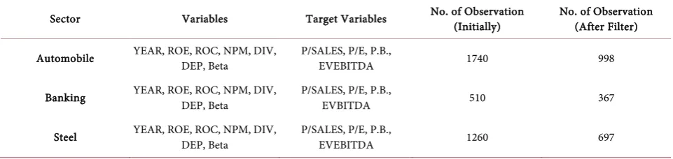
The number of initial observations taken were 3510 initially, however, after filtering, the final sample of firm observations came to be 2062 (Table 1).

3.2. Identification of Valuation Multiples and Their Fundamentals

The principal variables considered are:

• _{Price/Sales Ratio: Interpretable as ratio: (Stock price × No. of outstanding}

(8)

[image:8.595.59.540.90.204.2]

DOI: 10.4236/tel.2019.91015 187 Theoretical Economics Letters Table 1. Companies for the study.

Sector Variables Target Variables No. of Observation _(Initially) No. of Observation _{(After Filter)}

Automobile YEAR, ROE, ROC, NPM, DIV, _{DEP, Beta} P/SALES, P/E, P.B., _EVEBITDA 1740 998

Banking YEAR, ROE, ROC, NPM, DIV, _{DEP, Beta} P/SALES, P/E, P.B., _EVBITDA 510 367

Steel YEAR, ROE, ROC, NPM, DIV, _{DEP, Beta} P/SALES, P/E, P.B., _EVEBITDA 1260 697

• _{EV/EBITDA Ratio or Enterprise Multiple: It is used as a valuation tool to}

compare the value of a company, debt included, to the company’s cash earn-ings less non-cash expenses.

• _{Price/Book Value: It is interpretable as a ratio of (Stock price × No. of}

out-standing shares)/(Sum of the book values of Equity and Debt of the compa-ny).

• _{Price/Earnings Ratio: Can be interpreted as ratio of Market Value of the}

company and the EPS. Indicates the amount an investor can expect to invest in the company in order to receive one rupee of that company’s earnings. The key drivers for each multiple are based on Gordon model (Gupta [1]).

3.3. Testing for Structured Data

It is necessary to ascertain whether data in its totality displays certain structure? From the point of predictive analytics this is an important issue. The more the data has a structure the better will it be for predictive analytics point of view. Today, in the machine learning domain, there are a number of visualization techniques that enable multidimensional structural information in two dimen-sions. Two such techniques that the author has used are Andrews plots and t-SNE. Both techniques use different approaches to transform multidimensional data to two dimensions and enable plotting. In both the cases, the presence or absence of structure is indicated by occurrences or absence of patterns in the plot. If certain patterns are discernible, data is structured, else not. From the Andrews plots for all three sectors i.e. Auto-sector, Banking Sector and Steel Sector, it can be seen that plenty of structural information is evident (Figure 1(b)). This is also true of t-SNE plots. These plots attest to the relevancy of data collected.

3.3.1. Andrew Curve Plot

(9)

displaying multivariate data have been suggested. One of the most appealing methods is that of Andrews Plots. Andrews Plots provide a means for the simul-taneous display of several continuous variables. An Andrews plot or Andrews curve is a way to visualize structure in high-dimensional data. We can represent high-dimensional data with a number for each of their dimensions, x = {x1, x2,

x3 … ad}.

Figure 1(a) represents the Andrews curve with unstructured data. According to the above equations there is a structure in the data, and this is visible in the Andrews’ curves of the data from Auto, Banking and Steel sectors (Figure 1(b)). In the plot above, each color used, represents a class and we can easily note that the lines that represent samples from the same class have similar curves.

3.3.2. T-SNE (t-Distributed Stochastic Neighbor Embedding)

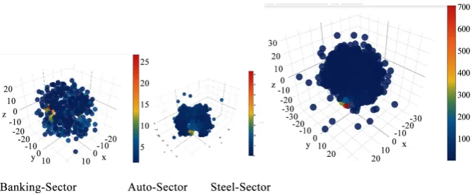
T-SNE visualizes high-dimensional data by giving each data point a location in a two or three-dimensional map. The technique is a variation of Stochastic Neighbor Embedding Hinton and that is much easier to optimize, and produces significantly better visualizations by reducing the tendency to crowd points to-gether in the center of the map (Roweis [24]). T-SNE is better than existing techniques at creating a single map that reveals structure at many different scales. T-SNE can use random walks on neighborhood graphs to allow the im-plicit structure of all of the data to influence the way in which a subset of the da-ta is displayed.

It can be reaffirmed from Figure 2 that the data for our study is struc-tured. Least outlier can be seen for Banking Sector followed by Auto Sector. The Steel Sector has more outliers as is visible from the plot above.

3.4. Missing Data

Few missing variables have been imputed. Imputation has been done using the industry standard method of MICE: Multivariate Imputation by Chained Equa-tions. Very briefly MICE employs the philosophy that while one may, in certain circumstances, use mean and median to supply missing variables to numeric da-ta considering values in a particular column (variable), but in its toda-tality a value

(10)

DOI: 10.4236/tel.2019.91015 189 Theoretical Economics Letters (b)

[image:10.595.261.483.65.527.2]

Figure 1. (a) Andrews curve with unstructured data; (b) Andrews curve for the three sectors. Source: Python Application.

[image:10.595.204.539.569.707.2]

(11)

in a column is also related to values in other columns. Thus, while imputing values it is better to develop a model that takes into account values of other re-lated variables and then imputes the missing value. For this reason, as of today MICE stands at the top of preferred methods for supplying missing values.

There were some missing data, for certain variables, and this can have a sig-nificant effect on the conclusions that can be drawn from the data.

Rubin [25] differentiated between three types of missing data mechanisms:

• _{Missing completely at random (MCAR): When cases with missing values can}

be thought of as a random sample of all the cases; MCAR occurs rarely in practice.

• _{Missing at random (MAR): When conditioned on all the data we have, any}

remaining missing value is completely random; that is, it does not depend on some missing variables. So missing value can be modelled using the observed data. Then, we can use specialized missing data analysis methods on the available data to correct for the effects of missing value.

• _{Missing not at random (MNAR): When data is neither MCAR nor MAR.}

This is difficult to handle because it will require strong assumptions about the patterns of missing data.

To handle the missing data, the following strategy was adopted:

• _{Imputed by Mean or Median: The methodology adopted was to find the}

correlation between the target variable and imputed predictor variable, after the predictor variable imputed either with mean or median. The missing data is imputed for those variables which resulted into significant correlation coefficient.

• _{MICE (Multivariate Imputation by Chained Equations): Imputing}

multiva-riate data using joint modelling (JM) and fully conditional specification (FCS). This involves specifying a multivariate distribution of missing data, and drawing imputation from their conditional distribution by Markov Monte Carlo (MCMC) techniques. FCS specifies the multivariate imputation model on a variable-by-variable basis by a set of conditional densities, one for each incomplete variable.

MICE Algorithm

Let the hypothetically complete data Y be a partially observed random sample from the p multivariate distribution P (Y|θ). We assume that the multivariate distribution of Y is completely specified by θ, a vector of unknown parameters. The problem is how to get the multivariate distribution of θ, either explicitly or implicitly.

The name chained equations refers to the fact that the MICE algorithm can be easily implemented as a concatenation of univariate procedures to fill out the missing data.

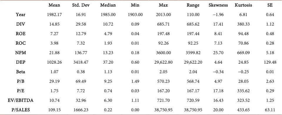
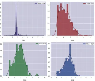
3.5. Testing for Skewness by Descriptive Statistics

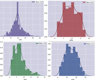
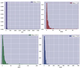
All variables are generally positively high-skewed in all the sectors (Tables 2-4;

(12)

[image:12.595.208.540.129.397.2] [image:12.595.209.538.429.705.2]

of the distribution of variables such as net profit margin (NPM), dividend payout (DIV), P/E, EV/EBITDA, P/Sales. In addition, the means of the multiples are greater than the medians, suggesting a positively skewed distribution.

Figure 3. Skewness of data for the Auto Sector. Source: Python Application.

(13)

[image:13.595.207.538.65.346.2] [image:13.595.57.541.398.607.2]

DOI: 10.4236/tel.2019.91015 192 Theoretical Economics Letters Figure 5. Skewness of data for Steel Sector. Source: Python Application.

Table 2. Descriptive statistics for Auto Sector.

Mean Std. Dev Median Min Max Range Skewness Kurtosis SE

Year 1977.29 16.48 1982.00 1901.00 2011.00 110.00 −1.33 3.45 0.52

DIV 17.94 11.99 15.90 0.26 89.02 88.76 1.49 3.89 0.38

ROE 11.67 9.38 9.57 0.16 72.75 72.59 1.98 6.36 0.30

ROC 5.03 3.78 3.93 0.05 25.56 25.51 1.20 1.53 0.12

NPM 27.04 22.54 23.73 0.48 316.36 315.88 5.21 48.80 0.71

DEP 767.58 2408.43 141.90 1.80 28,202.00 28,200.20 6.78 54.71 76.24

Beta 0.90 0.28 0.89 0.10 2.05 1.95 0.21 0.89 0.01

P/B 22.07 62.29 12.21 1.39 1182.74 1181.35 12.16 175.61 1.97

P/E 2.34 2.54 1.57 0.03 29.77 29.74 3.90 24.92 0.08

EV/EBITDA 7.71 6.82 5.97 −1.96 83.45 85.41 3.90 25.62 0.22

P/SALES 1.22 3.79 0.45 0.00 92.08 92.08 15.94 345.04 0.12

Table 3. Descriptive statistics for Banking Sector.

Year 1947.40 36.76 1936.00 1865.00 2014.00 149.00 0.16 −1.08 1.92

DIV 19.17 6.96 19.40 0.03 46.74 46.71 0.32 0.74 0.36

ROE 14.41 6.31 14.16 1.48 31.56 30.08 0.11 −0.75 0.33

[image:13.595.57.540.640.728.2]

(14)

DOI: 10.4236/tel.2019.91015 193 Theoretical Economics Letters Continued

NPM 9.36 4.09 9.42 1.15 17.94 16.79 0.01 −0.94 0.21

DEP 1356.90 2055.39 670.30 15.30 17,003.10 16,987.80 3.65 16.50 107.29

Beta 1.19 0.28 1.14 0.45 2.01 1.56 0.43 −0.20 0.01

P/B 1.56 1.22 1.22 0.35 10.97 10.62 2.74 11.80 0.06

P/E 14.63 15.36 9.21 1.97 170.02 168.05 4.57 33.49 0.80

EV/EBITDA 2.12 3.26 0.92 0.01 26.78 26.77 3.66 17.53 0.17

[image:14.595.59.539.233.428.2]

P/SALES

Table 4. Descriptive statistics for Steel Sector.

Year 1982.17 16.91 1985.00 1903.00 2013.00 110.00 −1.96 6.81 0.64

DIV 14.85 29.58 10.72 0.09 685.71 685.62 17.41 380.33 1.12

ROE 7.27 12.79 4.79 0.04 197.48 197.44 8.41 94.48 0.48

ROC 3.98 7.32 1.93 0.01 92.26 92.25 7.13 70.86 0.28

NPM 21.88 136.77 13.23 0.18 3600.00 3599.82 25.70 669.09 5.18

DEP 1028.26 3418.47 37.20 0.60 29,622.80 29,622.20 4.64 24.85 129.48

Beta 1.07 0.38 1.13 0.01 2.05 2.04 −0.34 −0.25 0.01

P/B 29.19 69.49 9.25 1.49 570.23 568.74 4.97 28.05 2.63

P/E 1.75 7.72 0.74 0.03 167.20 167.17 17.18 335.62 0.29

EV/EBITDA 10.74 32.96 6.30 1.11 721.70 720.59 16.43 323.52 1.25

P/SALES 109.15 1666.23 0.22 0.00 38,750.95 38,750.95 20.00 433.65 63.11

3.6. Transformation

All explanatory variables in different sectors are highly positively skewed due to presence of outliers. We have imposed following steps to deal with skewness and outliers respectively:

1) Transform data from x to log (1 + x). 2) Trim Outliers with mean or median.

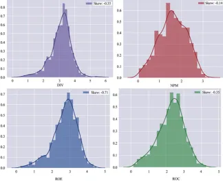
When we have transformed the data according to above two methods, skew-ness of data has decreased, explanatory variables distributed normally (Figures 6-8).

3.7. Feature Engineering

The complex models are difficult to interpret as also, tougher to tune. Simple algorithms and models, with good features or large data give far better results than a weak assumption accompanied with a complex model. A good feature implies flexibility, simpler in nature and good accuracy result giving model. Presence of irrelevant features can effect negatively during generalization of re-sults. So, feature selection and feature engineering are the most two important things for running any model.

(15)

[image:15.595.211.536.130.394.2] [image:15.595.210.538.426.705.2]

features from leveraging the existing explanatory variables in the given set of da-ta, due to which it increases the predictive power of existing model or model ac-curacy.

Figure 6. Auto Sector explanatory variables (after transformation).

(16)

DOI: 10.4236/tel.2019.91015 195 Theoretical Economics Letters Figure 8. Steel Sector explanatory variables (after transformation). Source: Python Application.

We have created the following features from leveraging existing predictor va-riables:

• _{Interaction Effects (}_{Table 5}_{): Created 15 new features from the product of}

two existing different predictor variables.

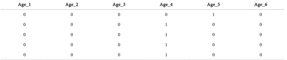
• _{Dummy Variable (}_{Table 6}_{): Created 6 new features from the existing}

cate-gorical predictor variable i.e. Year of Incorporation of Companies.

3.8. Regression Techniques

In contrast to the “comparable firms” approach, the information in the entire cross-section of firms can be used to predict valuation multiples. The simplest way of summarizing this information is with a multiple regression, with the multiple as the dependent variable, and proxies for risk, growth and payout forming the independent variables.

The Gordon Dividend Discount Model (DDM) is restated using accounting variables; we have substituted dividends with earnings and book value to rede-fine the expected price of a company’s stock as a function of the market’s expec-tations of future earnings (Damodaran) [26] [27].

Multiple Regression methodology suffers from constraints as:

 _{The basic regression assumes a linear relationship between multiples and the}

financial proxies, and that might not be appropriate.

 _{The basic relationship between multiples and financial variables itself might}

[image:16.595.214.536.66.340.2]

(17)

[image:17.595.58.539.89.192.2]

DOI: 10.4236/tel.2019.91015 196 Theoretical Economics Letters Table 5. Interaction effects among variables.

new_ROC_ROE new_NPM_ROE new_NPM_ROC new_DIV_ROE … new_Beta_DIV new_Beta_DEP

12.472409 11.738326 9.87647 9.349453 … 0.599459 0.689027

8.580828 6.119508 5.47977 6.962525 … 1.419847 3.245787

10.276659 7.157738 6.012539 5.786666 … 1.096358 3.646969

7.824396 5.44956 4.462748 6.955583 … 1.514286 3.935495

11.676866 8.485134 7.719118 9.895043 … 2.088338 4.58584

Table 6. Dummy variable coding for age as variable.

Age_1 Age_2 Age_3 Age_4 Age_5 Age_6

0 0 0 0 1 0

0 0 0 1 0 0

 _{The independent variables are correlated with each other. For example, high}

growth firms tend to have high risk. This multi-collinearity makes the coeffi-cients of the regressions unreliable and may explain the large changes in these coefficients from period to period.

To overcome the limitations of the linear regression approach, we have ap-plied the Ridge Regression, LASSO and Elastic Net regularization techniques.

3.8.1. Ridge Regression

Ridge Regression is a regression technique that overcomes the multi collinearity limitation of multiple regression. Multicollinearity technique leads to large va-riances which often lead to values which are not reflecting the true values.

• Method of producing a biased estimator of b that has a smaller Mean Square Error than OLS.

• Mean Square Error of Estimator = Variance + Bias2_.

• Ridge estimator trades of bias for large reduction of variance when the pre-dictor variables are highly correlated.

• Method of producing a biased estimator of b that has a smaller Mean Square Error than OLS.

• Mean Square Error of Estimator = Variance + Bias2_.

• Ridge estimator trades of bias for large reduction of variance when the pre-dictor variables are highly correlated.

The effect of this equation is to add a shrinkage penalty of the form where the tuning parameter λ is a positive value.

[image:17.595.58.543.228.329.2]

(18)

DOI: 10.4236/tel.2019.91015 197 Theoretical Economics Letters • _{Note that when}_λ_{= 0, the penalty term as no effect, and ridge regression will}

procedure the OLS estimates. Thus, selecting a good value for λ is critical (can use cross-validation for this).

• _As_λ_{increases, the standardized ridge regression coefficients shrink towards}

zero.

• _{Thus, when}_λ_{is extremely large, all of the ridge coefficient estimates are}

bas-ically zero; this corresponds to the null model that contains no predictors. Ridge Regression Models

In ridge regression, the first step is to standardize the variables (both depen-dent and independepen-dent) by subtracting their means and dividing by their stan-dard deviations. Ridge regression calculations are based on stanstan-dardized va-riables. When the final regression coefficients are displayed, they are adjusted back into their original scale. However, the ridge trace is in a standardized scale.

The linear regression gives an estimate which minimizes the sum of square error.

Y X B e= × +

Where, Y is the dependent variable, X represents the independent variables, B is the regression coefficients to be estimated, and e represents the errors are resi-duals.

The ridge regression gives an estimate which minimise the sum of square er-ror as well as satisfies the constraint that 2

1

P j

j=

β

≤c

∑

(

)

1 0 1 1 2 2 ^ 2 n

i

Min

∑

₌ yi−β +β × iβ ×

Subject to

2 2 1 j j=β β≤s

∑

By using Lagrange multiplier, we can write the above equation as, where, both λ and s are constant and the above equation in matrix form:

(

) (

)

Min_Y₋_βT_X T _Y₋_βT_X

Ridge regression has two important advantages over the linear regression. The most important one is that it penalizes the estimates. It doesn’t penalize all the features’ estimate arbitrarily. If estimates (β) values are very large, then the SSE term in the above equation will minimize, but the penalty term will increase. If estimates (β) values are small, then the penalty term in the above equation will minimize, but, the SSE term will increase due to poor generalization. So, it chooses the feature’s estimates (β) to penalize in such a way that less influential features (some features cause very small influence on dependent variable) un-dergo more penalization. In some domains, the number of independent vari-ables is many, as well as we are not sure which of the independent varivari-ables in-fluences the dependent variable. In this kind of scenario, ridge regression plays a better role than linear regression.

(19)

DOI: 10.4236/tel.2019.91015 198 Theoretical Economics Letters X will be less than P + 1 (where P is number of regressors). So, the inverse of

XT_X_{doesn’t exist, thus the OLS estimate may not be unique.}

The ridge regression estimate is given by

(

_T

)

1 _T

ridge _X _X _I _{X Y}

β = × + ×λ −

For ridge regression, we are adding a small term λ along the diagonals of XT_X_.

It makes the XT_X₊_λI_{matrix to be invertible (all the columns are linearly}

inde-pendent).

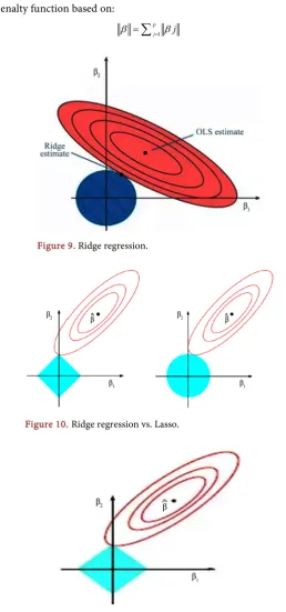
Ridge regression doesn’t produce unbiased estimate as linear regression. This is the contour plot of ridge regression objective function (Figure 9). The ridge estimate is given by the point at which the ellipse and the circle touch.

3.8.2. Lasso (Least Absolute Shrinkage Selector Operator)

LASSO helps us in getting better values of predictors as compared to even ridge regression.

It’s a version of the ordinary least square estimate by shrinking coefficients, by minimizing the Residual Sum of Squares subject to the constraint that the sum of the absolute value of the coefficients should be no greater than a constant.OLS estimates often have low biases but large variance, Lasso improves the overall prediction accuracy by sacrifice a little bias to reduce the variance of the pre-dicted value.

The key difference between ridge regression and lasso is that lasso uses an 1

penalty instead of an 2, which has the effect of forcing some of the coefficients

to be exactly equal to zero when the tuning parameter λ is sufficiently large. Thus, lasso performs variable/feature selection.

The lasso and ridge regression coefficient estimates are given by the first point at which an ellipse contacts the constraint region (Figure 10).

The merits of lasso are:

• _{Lasso has a major advantage over ridge regression, in that it produces simpler}

and more interpretable models that involve only a subset of predictors.

• _{Lasso leads to qualitatively similar behavior to ridge regression, in that as}_λ

increases, the variance decreases and the bias increases.

• _{It can generate more accurate predictions compared to ridge regression.} • _{Cross-validation can be used in order to determine which approach is better}

on a particular data set.

(20)

over other subset selection method (forward, backward regression) is that it uses convex optimisation to find out the best features. So, it converges faster com-pared to other methods.

3.8.3. Elastic Net

The elastic net method overcomes the limitations of the Lasso method which uses a penalty function based on:

1 p

j j

[image:20.595.238.497.156.709.2]

β =

∑

₌ β

Figure 9. Ridge regression.

Figure 10. Ridge regression vs. Lasso.

[image:20.595.267.479.182.490.2]

(21)

Use of this penalty function has several limitations. For example, in the “large p, small n” case (high-dimensional data with few examples), the Lasso selects at most n variables before it saturates. Also if there is a group of highly correlated variables, then the Lasso tends to select one variable from a group and ignore the others. To overcome these limitations, the Elastic Net adds a quadratic part to the penalty (||β2_{||) which when used alone is ridge regression (known also as}

Tikhonov regularization).

The quadratic penalty term makes the loss function strictly convex, and it therefore has a unique minimum (Figure 12). The elastic net method includes the Lasso and ridge regression: in other words, each of them is a special case where λ2 = λ or λ2 = 0 or λ1 = 0, λ1 = λ. Meanwhile, the naive version of elastic

net method finds an estimator in a two-stage procedure: first for each fixed it finds the ridge regression coefficients, and then does a Lasso-type shrinkage. This kind of estimation incurs a double amount of shrinkage, which leads to in-creased bias and poor predictions. To improve the prediction performance, the authors rescale the coefficients of the naive version of elastic net by multiplying the estimated coefficients by (1 + λ2).

4. Empirical Findings

4.1. Prediction Errors Using RMSE and Learning Curves

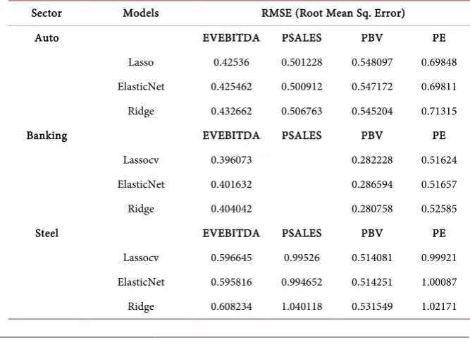
Root Mean Squared Error (RMSE): It is the square average over the test sample of the absolute differences between prediction and actual observation where all individual differences have equal weight. In other words, RMSE is the square root of the variance of the residuals (Table 7).

[image:21.595.204.538.499.742.2]

The RMSE of a model prediction with respect to the estimated variable X-model is defined as the square root of the mean squared error:

Table 7. RMSE for the four multiples across the three sectors.

Sector Models RMSE (Root Mean Sq. Error)

Auto EVEBITDA PSALES PBV PE

Lasso 0.42536 0.501228 0.548097 0.69848 ElasticNet 0.425462 0.500912 0.547172 0.69811 Ridge 0.432662 0.506763 0.545204 0.71315

Banking EVEBITDA PSALES PBV PE

Lassocv 0.396073 0.282228 0.51624

ElasticNet 0.401632 0.286594 0.51657

Ridge 0.404042 0.280758 0.52585

Steel EVEBITDA PSALES PBV PE

(22)

[image:22.595.218.516.65.467.2]

DOI: 10.4236/tel.2019.91015 201 Theoretical Economics Letters Figure 12. Elastic net technique.

2 , , 1( ) n

obs i model i

i X X

RMSE

n

= −

=

∑

where Xobs = observed values.

Xmodel = modelled values.

n = number of observation. Learning Curves

Learning curves are one of the methods through which we can observe the over-fitting or under-fitting effect on the training set and the effect of the train-ing size on the accuracy. A learntrain-ing curve shows the validation and traintrain-ing score of an estimator for varying numbers of training samples. It is a tool to find out how much we benefit from adding more training data and whether the esti-mator suffers more from a variance error or a bias error. If both the validation score and the training score converge to a value that is too low with increasing size of the training set, we will not benefit much from more training data.

We will probably have to use an estimator or a parameterization of the current estimator that can learn more complex concepts (i.e. has a lower bias). If the training score is much greater than the validation score for the maximum num-ber of training samples, adding more training samples will most likely increase generalization.

1) Auto Sector (Figure 13) 2) Banking Sector (Figure 14) 3) Steel Sector (Figure 15)

(23)

[image:23.595.209.534.131.301.2] [image:23.595.212.537.334.506.2]

which indicates that the result from the given model can be generalized. We also observe that when learning curves are generated by all the three techniques (ridge, lasso and elastic net) our results are similar and the curves for all the

[image:23.595.208.538.339.700.2]

Figure 13. Learning curves Auto Sector-P/SALES. Source: Python Application.

Figure 14. Learning curves Banking Sector-P/BV.

[image:23.595.212.540.538.703.2]

(24)

three models converge approximately at same point.

We thus conclude that both by looking at RMSE as also learning curves, P/S multiple explains auto sector best; P/BV the banking sector and EV/EBIDTA the steel sector.

4.2. Key Fundamental Drivers for Each Multiple

It can be seen from Figure 16 that for auto sector, Net profit margin (NPM) with depreciation, (interaction effect) and NPM with ROC are the key drivers. We thus see that the fundamental financial variables that are significant for this sector are NPM, ROC and some interaction effects.

It can be observed from Figure 17 that when all the explanatory variables are taken, the significant variables for this sector are return on equity, age of the company and the interaction effects of ROE with depreciation and ROE with dividends.

Figure 18 shows that based on the three techniques for our research, age of the company, dividend pay-out ratio, interaction of dividend with NPM, beta with ROE, and ROC are the significant variables.

5. Conclusions

The objective of this research paper has been to use a parsimonious model for testing the predictive accuracy of valuation multiples. The author has hig-hlighted the limitations of the traditional regression techniques, including nor-mality and multi collinearity, and has thus applied regularization techniques of ridge regression, Lasso and Elastic Net to evaluate the best fit multiple for three sectors: automobile, banking and steel.

Applying ridge regression not only is the constraint of multi-collinearity re-solved, but also minimizes MSE (mean square errors). However, since it shrinks the coefficients to zero, it cannot produce a parsimonious model. To reduce the complexities of ridge regression, Lasso regression is also applied. Lasso is very similar to Ridge regression. The only difference being the penalty that is added to the *least squares objective function. This regression also has limitations in that when we have correlated variables, it retains only one variable and sets other correlated variables to zero. That will possibly lead to some loss of information resulting in lower accuracy in our model. Thus, research study has additionally used Elastic net which overcomes the limitations of the other two methods in that there is no limit to the number of selected variables here and it encourages grouping effects in the presence of highly correlated predictors. Overall, Elastic Net combines the merits of both Ridge regression and Lasso.

(25)

[image:25.595.218.526.66.709.2]

(26)

[image:26.595.224.525.65.710.2]

(27)

[image:27.595.211.535.69.700.2]

(28)

have been converted to dummy variables.

With variables aplenty, a good predictive model is one which is able to dis-tinguish between chaff from wheat. Machine learning offers some choices in this regard from simple to regularized regression techniques. The techniques identi-fied and selected are the three best available regression techniques: Ridge, LASSO and Elastic Net. These three methods offer different ways to regularize a model. Regularization is a way to constrain the complexity of a model and keep it as generalizable as possible to unseen data. It filters out those variables that may be noisy or unimportant. There is an attempt to create a predictive model as is evident from learning curves. Learning curves give an indication how good and generalizable a model is. Finally, the author has listed the most important features that help in making accurate predictions. This feature importance comes as a by-product of regression analysis. It is evident from the empirical findings that by and large all the three modeling techniques agree to the set of most important features.

This study contributes to the existing literature on Indian economy by identi-fying the multiples which explain the valuations of these three sectors best. This can help investors in deciding on their investment in securities markets and can also help in equity research. The predicted multiples can be compared to the multiples at which the stocks are currently trading and help in buy/sell decisions for investors, both retail and institutional. Identifying the key fundamental driv-ers for each sector also helps in providing a pdriv-erspective on the future outlook and prospects of firms within a sector. These accounting variables can also help in subsequent valuations of unlisted private firms. Our research contributes to practitioners, such as investment bankers and analysts, hedge funds and private equity, and also to academic researchers.

Limitations of the Study

The research uses historical data and the prediction accuracy may change when predicted earnings or other variables are considered. The results are based on statistical analysis, and we have not factored in comparable companies based on benchmarking. The results may differ if we use that approach. The benchmark method is relevant when valuing private and unlisted firms. While the data is taken for 12 years, increasing the time span may also give different results.

Scope of Future Research

The limitations of this research study can give us direction for future research. The analysis can be done based on forecasted numbers instead of historical data. Re-searchers can also use other sources of information as database of analysts. We can widen the scope by factoring in other multiples, in addition to the four taken for the study and expand our dataset of companies to beyond these three sectors.

Acknowledgements

(29)

research paper.

Conflicts of Interest

The author declares no conflicts of interest regarding the publication of this pa-per.

References

[1] Gupta, V. (2018) Predicting Accuracy of Valuation Multiples Using Value Drivers: Evidence from Indian Listed Firms. Theoretical Economics Letters, 8, 755-772. [2] Jenkins, D. (2006) The Benefits of Hybrid Valuation Models. The CPA Journal. [3] Alford, A.W. (1992) The Effect of the Set of Comparable Firms on the Accuracy of

Price Earnings Valuations Method. Journal of Accounting Research, 30, 94-108. [4] Penman, S. (1998) Combined Earnings and Book Value in Equity Valuations.

Con-temporary Accounting Research, 15.

[5] Liu, J., Nissim, D. and Thomas, J. (2002) Equity Valuation Using Multiples. Journal of Accounting Research, 40, 135-172. https://doi.org/10.1111/1475-679X.00042

[6] Yoo, Y.K. (2006) The Valuation Accuracy of Equity Valuation Using a Combination of Multiples. Review of Accounting and Finance, 5, 108-123.

[7] Antonios, S., Ioannis, S. and Panagiotis, A. (2012) Equity Valuation with the Use of Multiples. American Journal of Applied Sciences, 9, 60-65.

[8] Nel, W.S. (2009) The Use of Multiples in the South African Equity Market: Is the Popularity of the Price Earnings Ratio Justifiable from a Sector Perspective? Medi-tari Accountancy Research, 17, 101-115.

[9] Nel, W.S. and Roux, N.J. (2015) An Analyst’s Guide to Sector-specific Optimal Peer Group Variables and Multiples in the South African Markets. Economics, Manage-ment, and Financial Markets, 12, 25-54.

[10] Schreiner, A and Spremann, K. (2007) Multiples and Their Valuation Accuracy in European Equity Markets. https://doi.org/10.2139/ssrn.957352

https://ssrn.com/abstract=957352

[11] Nissim, D. (2013) Relative Valuation of U.S. Insurance Companies. Review of Ac-counting Studies, 18, 324-359.

[12] Knudsen, J.O., Kold, S. and Plenborg, T. (2017) Stick to the Fundamentals and Dis-cover Your Peers. Financial Analysts Journal, 73, 85-105.

[13] Bhargava, M. (2014) Factors Influencing Pricing Multiples in India. The IUP Jour-nal of Applied Finance, 20.

[14] Dasanayaka, S.W. (2014) Investors Behavior in Stock Exchanges Based on Price Multiples and Value Drivers: A Case Study Based on Colombo Stock Exchange in Sri Lanka. Global Management Journal for Academic & Corporate Studies, 4. [15] Lie, E. and Lie, H.J. (2002) Multiples Used to Estimate Corporate Value. Financial

Analysts Journal, 58, 44-54.

[16] Zahir, M.A. and Khanna, Y. (1982) Determinants of Stock Prices in India. The Chartered Accountant, 30, 521-523.

[17] Kumar and Hundal (1986) Stock Market Integration Examining Linkages between India and Selected Asian Markets. Foreign Trade Review, 45, 3-18.

(30)

DOI: 10.4236/tel.2019.91015 209 Theoretical Economics Letters 31-65.

[19] Holland, P. (1973) Weighted Ridge Regression: Combining Ridge and Robust Re-gression Methods. NBER Working Paper Series, Cambridge.

[20] Saleh, A.K., Kibria, E. and Golam, B.M. (2013) Improved Ridge Regression Estima-tors for the Logistic Regression Model. Computational Statistics, 28, 2519-2558.

https://doi.org/10.1007/s00180-013-0417-6

[21] Zang, T. and Yang, B. (2017) An Exact Approach to Ridge Regression for Big Data.

Computational Statistics, 32, 909-928.https://doi.org/10.1007/s00180-017-0731-5

[22] Kubus, M. and Folia, O.S. (2016) Assessment of Predictor Importance with the Example of the Real Estate Market. Szczecin, 16, 29-39.

https://doi.org/10.1515/foli-2016-0023

[23] Chen, J. and Tindall, M.L. (2014) Hedge Fund Replication Using Shrinkage Me-thodologies. The Journal of Alternative Investments, 17, 26-49.

https://doi.org/10.3905/jai.2014.17.2.026

[24] Roweis, S. and Hinton, G. (2002) Stochastic Neighbor Embedding. Proceedings of the 15th International Conference on Neural Information Processing Systems, 857-864.

[25] Rubin, D. (1976) Inference and Missing Data. Biometrika, 63, 581-592.

https://doi.org/10.1093/biomet/63.3.581

[26] Damodaran, A. (2005) Valuation Approaches and Metrics: A Survey of the Theory and Evidence. Now Publishers, Hanover.