Simulation Vacuum Preloading Method by Tri Axial Apparatus

Simulation Vacuum Preloading Method by

Tri-Axial Apparatus

Ngo Trung Duong1, Wanchai Teparaksa1, Hiroyuki Tanaka2

1_{Department of Civil Engineering, Faculty of Engineering, Chulalongkorn University, Bangkok, Thailand} 2_{Faculty of Engineering, Hokkaido University, Sapporo, Japan}

Email: ngotrungduong@yahoo.com, wanchai.te@chula.ac.th, tanaka@eng.hokudai.ac.jp

Received October 25,2011; revised December 14, 2011; accepted January 13, 2012

ABSTRACT

It is very important to control any risk of instability of embankment during vacuum construction, the simulation vacuum preloading method using tri-axial apparatus is proposed to predict the behavior of soft soil improvement in the labora-tory, as well as to make this method become familiar and easier in the future. The tri-axial apparatus is used instead of the large-scale one, which has been performed by Bergado (1998) and Indaratna (2008). The tri-axial test on small size specimen can be carried out in one week compared to the large-scale apparatus takes one month for big specimen. In addition, the lateral deformation as well as the shear strength increase with time can determine accurately.

Keywords: Soft Soil; Soil Improvement; Vacuum Preloading; Degree of Consolidation

1. Introduction

Nowadays the vacuum preloading consolidation method becomes the popular method to improve soft soil. This method is an effective method of improving soft soil conditions as introduced by Kjellman (1952) [1] in early 1952. With the merging of new materials and technolo-gies, this method has been further improved in recent years.

The modeling vacuum method to improve soft soil in the laboratory has been performed by Indaratna 2008 [2] using the large-scale apparatus and follows one-dime- nsional consolidation theory (Tezaghi). The results ob- tained from this modeling partially evaluated the behav- ior of soft soil reinforced by vacuum preloading method in the laboratory. Using the large specimen 45 cm × 90 cm in diameter and height respectively in the large-scale apparatus, the time used for this test was more than one month.

The horizontal deformation εr during the tested time,

which is the typical deformation of soft soil improvement by vacuum, and also the increasing of shear strength could not be measured. So far, the controlling surcharge processing during vacuum construction has not been discussed sufficiently.

The new method is proposed using tri-axial apparatus to simulate the comprehensive behavior of soil impro- vement by vacuum preloading method in the laboratory to support the engineering task quickly. In addition, it is desired to make the method become familiar in the

fu-ture.

The finite element method (FEM) is used to analyze two cases of drainage condition at the boundary and cen-ter of the axisymmetric soil cell.

The study aspects to solve these matters are as follows: 1) Simulation the behavior of soft soil improved by vacuum method by tri-axial apparatus under axisymetric consolidation condition;

2) The lateral deformation and vertical settlement are concerned during soil improvement by vacuum prel- oading method;

3) Evaluating the degree of consolidation during soil improvement;

4) Combination surcharge and vacuum preloading to estimate the increasing shear strength).

2. Tri-Axial Apparatus

Tri-axial apparatus can clearly evaluate the failure mech- anism as well as the capacity of increasing shear strength of soil in the laboratory. From the tri-axial test, the result parameters are used to predict the behavior of soil in the field during construction.

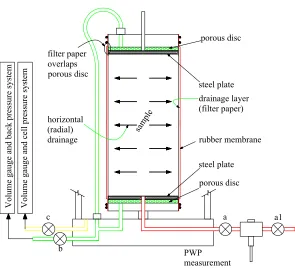
Under vacuum pressure condition alone, the soil mass at depth is subjected the isotropic stress status (K = 1). With flexible functions of the tri-axial machine as shown in Figure1, the isotropic condition of the soil mass can

generate the same vacuum condition by controlling the lateral earth pressure (K).

drainage layer (filter paper)

rubber membrane

porous disc

V

olum

e ga

ug

e an

d ba

ck

p

ressu

re

sy

ste

m

filter paper overlaps porous disc

horizontal (radial) drainage

V

olum

e ga

ug

e an

d ce

ll p

re

ssure system

PWP measurement

a c

b

sam ple

steel plate

a1 porous disc

steel plate

Figure 1. Scheme tri-axial apparatus.

be generating as axial force by the loading rod at top of the machine. The deformations of soil specimen in verti-cal and horizontal direction are measured during testing to evaluate the behavior of soil specimen.

The specimen is covered by rubber membrane and placed in the water tank; therefore the friction between circular soil specimen and the cell is eliminate, which is different to the oedometer apparatus.

The steel plates at the ends of specimen are as the im- pervious layer, only radial drainage is induced during consolidation. The filter paper covers around the bound- ary of specimen and overlaps the porous discs at the both ends of specimen as the drainage layer. For the large- scale oedometer apparatus, the drainage was established at the center of specimen. The FEM has been used to define the different between the drainage path conditions of specimen, and defines the correction factor for this simulation. The boundary conditions were illustrated in the Figure 2.

The assumptions were used for simulation of vacuum preloading method are as follow:

1) Soil mass as subjected vacuum pressure follows ax-isymmetric consolidation.

2) Under vacuum pressure only, soil mass will be sub-jected the Isotropic stress state, it mean that the coeffi-cient of horizontal earth pressure (K) equal to one, while for the surcharge only (K) value can calculate from Equation (1).

3) For the soil mass, the vacuum pressure is distributed along to the specimen is uniform.

H

De

H

De

(a) Drainage at center (b) Drainage at outer boundary

F

K 1 sinφ

igure 2. The drainage condition of axisymetric cell.

  (1)

where φ: the friction angle

3. Finite Element Method of Analysis for

3.1

drain

Nakanodo, 1974; Hansbo, 1981). Most researchers of soil.

Drainage Boundary Condition Analysis

. Thetheory of Asixmetric Consolidation

cepted that under embankment loading, the single drain analysis could not provide an accurate prediction due to lateral yield and heave compared to plane strain multi- drain analysis (Indraratna, et al., 1997) although the de- gree of consolidation (DOC) in this model is acceptable accuracy.

In this topic, the method is proposed to model the be-havior of soft soil improvement by vacuum combine with su

variation of the pe d-ar re Hooke’s la ring application. o (1

rcharge preloading method while the lateral displace-ment is concerned during consolidation.

The following assumptions are based on Hansbo solu-tion (1981) about equal strains (ε), the

rmeability (k) when void ratio (e) decrease during consolidation and the volume compressibility (mv).

1) Soil is homogeneous and fully saturated; the Darcy’s law is adopted. Depend on the purposes the outer boun

y of unit cell the drainage path is occurred.

2) Soil strain is uniform at the boundary of the unit cell and the small strain theory is valid, therefo

w should be applied for calculation.

3) For the mass soil, the vacuum pressure distribution along to the drain boundary is uniform du

The accuracy of the FE analysis was checked against the analytical solutions of Barron (1948) and Hansb

981) [3]. According to Barron (1948) [4], the degree of consolidation U for “equal-strain” consolidation is given in Equation (2).

8T U 1 exp

μ

 

  _ _

  (2)

with

2 2

2 2

n _{ln n} 3n 1

4n



  (3)

n 1

μ _ _

   e w D n D

 (4)

where De and Dw are diameters

lent of vertical drain respectively. Hansbo (1981) intro- of unit cell and equiva-

duced a circular smear zone (of diameter Ds) in the solu-

tion which resulted in a modified expression for μ

ho

k

n 3

ln ln m

m k 4

μ  _{ } 

  hs

(5) s w D m D

 (6)

For two dimensional consolida

pressed in terms of integrals of the excess pore water pr

tion U(%) can be

ex-essure over the unit cell domain as Madhav et al. 1993.

y x u(x, y,T)dxdy

 

 

where u(x,y,T) = excess pore water pressure at any point with x, y dimension at a time factor T, an

excess pore water pressure.

Terzaghi-Rendulic proposed differential equation for d uo is the initial

two-dimensional consolidation as

2 2

2 e

u u u

d  

  

 _{ 2 2}

T x y

 _  _ (8)

h

C t T ₂

e

D (9) where

Ch: horizontal coefficient of consolidation.

As the strains are small, if E'

effective stress, n' is Poisson’s ratio for effective stress material is isotropic, Hooke’s law is

is Young’s modulus for

and the

r r

θ r

r z

1 _{' 1 ' '}

E '

' ' 1 '

δε ν ν δσ

ν ν δσ

δε

'

1 ' '

δε ν ν δσ

      _ _{ }          _{ }        (10)  where:

{r, q, z} is the principal axes set.

{εr, εq, εz} are the strain in radial, circumferential and

vertical respectively.

oefficient of consolidation Ch in the horizontal

di train deformation is

sh The c

rection for axisymmetric plane s owed as:











h

w w

' E ' k k C

1 ' 1 2 ' mv

ν

ν ν γ γ

 

  (11)

where

1

kh: horizontal hydraulic conductivity

w: unit weight of water

Dummy research, for the axisymetric unit cell the co-t of volume compressibilico-ty (mv) varies during

co ression:

efficien

nsolidation; mv value calculate by exp

v a Δ m Δ v ε σ 

 (12)

where:

v: volume strain of specimen

σ'a: is the axial effective stress

of consolidation.

3.2 nit Cell under

stem of clay unit cell is used to model

re-T 7.5 cm × 15.0 cm in diameter

κ = 0.06, the horizontal and vertical at time reach to degree

. Solution for Axisymetric U Vacuum Pressure

An axisymetric sy

the behavior of soil specimen improved by vacuum p loading method.

he unit cell with size

(De) and height (H) respectively (H = 2D), the effective

Young’s modulus E' = 500 kN/m2_{, Poisson’s ration v' =}

hy

veral research-er

ell under vacuum pr

y FEM with Camclay Model, which sh

draulic coefficient kh = kv = 4.66E–10 m/sec and the

ratio n = De/Dw from 10, 20 are used to analyze. Dw is

equivalent diameter of vertical drain as in the Figure 3.

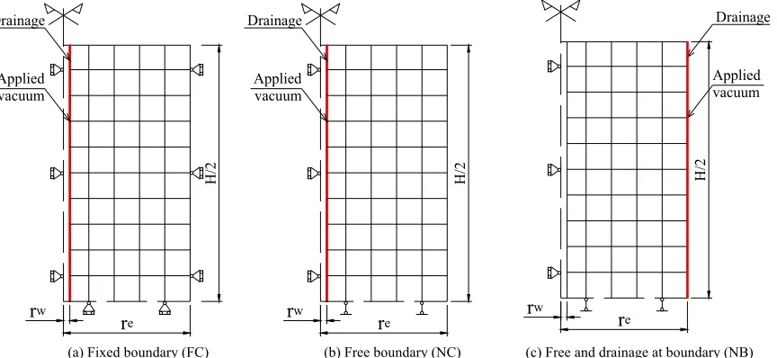
Three cases of axisymetric unit cells under vacuum preloading only as the Figure 3 were conducted to verify

the relationship about degree of consolidation in the dif-ferent boundary and drainage condition.

The first case, the outer boundary is fixed and drainage occurs at the center (FC) of unit cell. This is the conven- tional model to estimate the consolidation of axisymetric unit cell, which has been conducted by se

s before such as Indraratna (2005) [5], Chai (2006) [6], Tran (2007) [7]. One-dimensional consolidation theory is used for this case. As we know that, this case is very suitable for both cases the surcharge loading only and the

vacuum zone is infinite. Therefore, this method should not apply well for vacuum preloading.

The second and the third case are proposed to verify the consolidation of axisymetric unit c

eloading in term of the lateral displacement as well as two-dimensional consolidation is concerned, the outer boundary of specimen is free or none (N) combines drai- nage condition at the center (NC) and the outer boundary of unit cell (NB).

The series of case studies for axisymetric unit cell were conducted b

own in the Table 1. The cases from N1 to N12 are to

check the accuracy of FEM analysis with vary ratio (n) in 10 and 20 with vacuum pressure applied of 50 kPa and 100 kPa respectively.

rw

re

H/2

rw

re

H/2

Drainage Drainage

Applied

vacuum Appliedvacuum

Drainage

Applied vacuum

rw

re

H/

2

(a) Fixed boundary (FC) (b) Free boundary (NC) (c) Free and drainage at boundary (NB)

Figure 3. The modeling of axisymetric cell.

Ta ll.

N0 Case Bou Vacuum pressure (kPa) DOC (U%)

ble 1. The case studies for axisymetric unit ce

ndary condition Drainage condition Ratio De/Dw

N1 FC-1-50 Fixed Center N2 N

B

B

n = 20

50 100%

B

n = 10

B

n = 20

100 100%

U = 70% U = 40% B

B

C-1-50 Free (None) Center N3 NB-1-50 Free oundary

n = 10

N4 FC-2-50 Fixed Center N5 NC-2-50 Free Center N6 NB-2-50 Free oundary

N7 FC-1-100 Fixed Center N8 NC-1-100 Free Center N9 NB-1-100 Free oundary

N10 FC-2-100 Fixed Center N11 NC-2-100 Free Center N12 NB-2-100 Free oundary N13 NC-2-50-1 Free Center N14 NC-2-50-2 Free Center

N15 NB-2-50-1 Free oundary U = 70% N16 NB-2-50-2 Free oundary

n = 20 50

esult pr relationship between three cases

bo and d ndition of sp n. (FC), (NC

n

The r esents the

undary rainage co ecime )

a d (NB). The other cases (case N13 to N16) are to esti- mate applicable surcharge preloading during vacuum procedure.

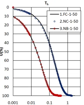
Comparisons were made for the cases of fix and none fix the outer boundary with ratio n = 10, n = 20 and vac-uum pressure only Va = 50 kPa, Va = 100 kPa. The re-sults of DOC (U%) and Time factor Th from the FEM

were found to compare well with the analytical solutions Baron (1948) [4] as show in the Figures 4-7.

The maximum difference in U, for U > 50%, was about 0.26%, occurring at T = 0.5 for the case n = 10 as shown in Figures 4 and 6. Forthe case n = , the maxi-20 mum difference in U was 0.17%, occurring at T = 0.5 as shown in Figures 5 and 7.

Conclusion the degree of consolidation in both cases fixed boundary (FC) and free boundary (NC) are almost sam

Figure 6. Case n = 10, vacuum only; Va = 100 kPa.

e value and agree strongly with Baron’s theory (1948).

Figure 7. Case n = 20, vacuum only; Va = 100 kPa.

For the cases none outer boundary and drainage at the outer boundary (NB), degree of consolidation e almost same in both case n = 10 and n = 20 as during vacuum

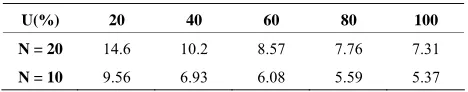
The Figure 8 and Table 2 show the relationship be-

tween the modeling of axisymetric unit cell in free boundary condition, drainage at the center (NC) and at the boundary (NB) during vacuum stage.

As the same DOC, the average ratio of time factor for drainage at the center and outer boundary is ThNC/ThNB

about 6.7 and 9.7 for n = 10, and n = 20 respectively as showed from case N01 to N12.

The consolidation procedure of unit cell in (NB) case is faster than (NC) case by ratio (ThNC/ThNB). The differ-

ent values relative to (n) ratio are shown in the Table 2.

The average coefficient of consolidation (Ch) in both

case (NC) and (NB) were found the same value and in-depe

Figure 4. Case n = 10, vacuum only; Va = 50 kPa.

ar

preloading.

ndent with (n) ratio, ChNC = ChNB ~ (2/3)ChFC.

3.

idation induced by vacuum pressure.

3. Solution for Axisymetric Unit Cell under Vacuum Combine Surcharge Loading

In this solution, the surcharge is applied after some de-gree of consol

Figure 8. Ratio of time factor ~U(%) for vacuum stage only.

Table 2. The ratio of time factor.

U(%) 20 40 60 80 100

N = 20 14.6 10.2 8.57 7.76 7.31

N = 10 9.56 6.93 6.08 5.59 5.37

Normally, the prefabricated vertical drain (PVD) of dimensions 10 cm × 0.4 cm is installed by rectangular shape. For this research the equivalent diameter of verti-cal drain Dw = 5 cm and diameter of cell De = 100 cm were

used. The example with De = 7.5 cm and Dw = 0.3875 cm,

and n = 20, were used in this analysis and shown in Fig-ure 9. This unit cell also used for modeling the vacuum

preloading in the laboratory test.

The surchage stages are applied in three cases of the degree of consolidation (U) reach to 40%, 70% and 100% as shown in the Table1.

onsolidat nd stage

is surcharge preloading during the vacuum is maintained. agni e and of lo g dete ned b

th asin effec tres oil m

rch load stim equa 80% of

in-rease vertical effective stress to prevent the failure state, o

factor T

There are two stages for vacuum preloading method, e first stage is vacuum preloading only until the degree th

of c ion reach to the target, and the seco

The m tud rate adin rmi ase on

e incre g of tive s s of s ass.

The su arge ing e ates l to

c

f r each case the loadings are 19.8 kPa, 29.6 kPa and 42.4 kPa respectively when 50 kPa vacuum pressure is applying.

The loading rate is 0.5 kPa/min for drainage at the cen- ter case (NC), the ration ThNC/ThNB are used from the Ta-

ble 2, of 10.2; 8.16 and 7.31 as degree of consolidation

40%; 70% and 100% respectively to define the loading rate when the drainage at outer boundary (NB).

The results of relationship between DOC (U) and time are shown from the Figures 10-12:

h

rw

re

H/

2

Drainage

Applied vacuum

rw

re

H/

2

Drainage

Applied vacuum

Surcharge Surcharge

(a)Drainage at center (b) Drainage at outer boundary

Figure 9. Vacuum combine surchage preloading.

Figure 10. Case n = 20, vacuum combine surchage loading V

; a = 50 kPa, U = 40%; ThNC/ThNB = 8.65.

Figure 12. Case n = 20, vacuum combine surchage loading; Va = 50 kPa, U = 100%.

average of ratio of time factor are equal to 8.71 & 8.65 for vacuum pres-sure are 100 kPa and 50 kPa respectively, when U = 100% the ratio of time factor is nearly same value 7.4.

In the Figure 14, degree of consolidation at 70%, the

maximum different in volume strain is 1.75% occuring at 420 min for case 40% is almost the same in the Figure 15.

From the analyzing above, the final volume strain in case outer boundary is almost same value as that in drainage at the center as surcharge applied at 40%; 70% and 100%.

Under vacuum 50 kPa and surcharge was applied as degree of consolidation is 100%, the Figure 16 showed

the deformation of unit cell (volume strain εv) during

time of vacuum and vacuum combine surcharge are same in two cases (NC) and (NB) after adjustment with the ratio of time factor ThNC/ThNB.

.98 during the surcharge was apply. These results are go

c-cu

ar

4.

From the Figure 13 and Table 3 the

The strain ration εr/εa are the same in both cases and

vary from 4 to 1.3 during vacuum stage and reduce to 0

od agreement with vacuum preloading theory, the lat-eral deformation of embankment is internal during ap-plying vacuum pressure.

The maximum different in volume strain is 2.13% o rring at 350 min while the final volume strain is the same in 13.24 (%).

These results also agree strongly with the solution in ticle 2. To make this solution more effectively, the laboratory test by Tri-axial apparatus should be carried out to support this research.

Simulation in Laboratory Test

4.1. Soil Specimen

The serial tests were performed by tri-axial apparatus in

Figure 13. Ratio of time factor surchage preloading.

~U(%) for vacuum combine

vacuum com- g.

Table 3. The ratio of time factor for n = 20, bine surchage preloadin

U(%) 20 40 60 80 100

100 kPa 9.33 9.31 9.16 8.41 7.32

50 kPa 9.10 8.70 8.63 8.17 7.41

8.71.

Figure 14. Case n = 20, vacuum combine surchage; Va = 50 kPa, U = 70%; ThNC/ThNB =

Figure 16. Case n = 20, Vacuum combine surchage; Va = 50 Pa, U = 100%; ThNC/ThNB = 7.31.

the laboratory in Hokkaido University to simulate the behavior of Akasaoka clay improved by vacuum prelo- ading method. The specimens of clay in sizes 75 mm × 150 mm in diameter and height respectively were used for this research, the specimens is suitable to control consolidation time under vacuum condition by tri-axial apparatus, also the retrieved samples from the field. For dummy research specimens were remodel in the labora-tory from the commercial Akasaoka clay powder.

The reconstituted Akasaoka clay was pre-consolidated under a pressure of 100 kPa and OCR = 1.25, e

physi-ard odometer test result. The pre-consolidated condition, the effective vertical stress and the effective horizontal stress are 80 kPa and 40 kPa respectively (the coefficient of horizontal earth pressure at rest K0 = 0.5).

Series conventional tri-axial test were carried out to verify the failure line (Kf) and relationship between the

coefficient K and the ratio su/σv' as show in Figure 18.

4.2. Test Procedure

Before application vacuum pressure, the specimen is saturated with B value more than 0.98 and reach to the initial pre-compression stress with effective vertical and horizontal stress are 80 kPa and 40 kPa respectively after

ted by applying the ef-ctive stress target with the lateral earth ratio equal to

k

th

cal properties of soil are listed in the Table 4 and Figure 17. The permeability coefficient (k) and compression

index (Cc) deduced from the stand

24 hours (Step loading and recompression step). The vacuum pressure is simula

fe

one (K = 1), the soil specimen is subjected the same con-dition under vacuum pressure as the period research, the behavior of soil mass under surcharge and vacuum pres-sure is shown in the Figure 19.

While the effective stress is applied, the drainage vale is clocked, under the undrained condition the excess pore water pressure has been increasing up to the vacuum

Table 4. Akasaoka clay’s properties.

Soil properties Values

Unit weight (kN/m3_{) 17.5}

Water content, w (%) 46.5 Liquid limit, wL (%) 62 Plastic limit, wP (%) 27.5 Plasticity index, PI (%) 34.5 Specific gravity, Gs 2.67 Initial void ratio eo 1.17

Figure 17. Void ratio ~log(p') graph.

F hear strength by effective str d ear-

t

igure 18. Predict s ess an

h ratio.

pressure desired. In the dummy research vacuum pres- sure, desired are 50 kPa and 100 kPa to concern the dep- ths of specimen there for the total vertical effective stress target of 130 kPa and 180 kPa were generating. (Vacuum pressure supplying step). The parameters in vacuum pro-ceed by tri-axial apparatus are shown in the Table 5.

The coefficient of horizontal earth pressure (K) is the ratio of the effective horizontal earth pressure due to the confinement from the surrounding soil mass to the verti-cal effective stress. Then from the Figure 20, K value

can be calculated as follows:

3 va 1 va ' ' K ' ' σ σ σ σ  

 (13)

During ation has

een occurred due to the excess pore water is dissipated, the effective stress of soil as well as the shear strength will be increase, this behavior is suitable with the vac- uum mechanism, and the tri-axial apparatus’s gauges record the behavior data and deformation of soil spe- cimen automatically. The soil is consolidated completely when the effective stress increase to the target and the excess pore water dissipates completely. However, from data from FEM and test the times of primary consolida- tion reach to as the excess pore water pressure dissipates about 95%.

Where:

CP: Cell pressure

Pore water pressure σv': Vertical effective stress target

σh': Horizontal effective stress target

K: Coefficient of horizontal earth pressure

The shearing steps are carried out to define the undra- ind shear strength of soil improved. Depend on the goals these step could be performed at the time after vacuum loading completely or with the increase of degree of consolidation reach to 40%, 70%, 100% combine with surcharge to estimate the capacity of soil embankment each construction stage respectively. This step is performed

drained progress stage, the consolid b

BP: Back pressure PWP: 75mm 15 0 m m '1  '3 =  '1 Pre-consolidated, OCR=1.25, k0=0.5 '1+'va  '3 +  'va Vacuum condition, 'va (kPa), K

Figure 20. Soil specimen under vacuum condition.

Table 5. Parameter in vacuum proceed by tri-axial appar- atus.

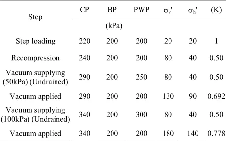
CP BP PWP v' h' (K)

Step

(kPa) Step loading 220 200 200 20 20 1 Recompression 240 200 200 80 40 0.50 Vacuum supplying

(50kPa) (Undrained) 290 200 250 80 40 0.50 Vacuum applied 290 200 200 130 90 0.692 Vacuum supplying

(100kPa) (Undrained) 340 200 300 80 40 0.50 Vacuum applied 340 200 200 180 140 0.778

to control the surcharge preloading at the site to avoid the so as the surcharge is over the soil capacity as

w e of embankment. The capacity of

so mulation (as empirical me-

th

il failed

ell as instability stag il can be predicted by for od Tanaka):

u u

S (s σv)*0.8* p (14) w

4.3. Test Results and Analysis

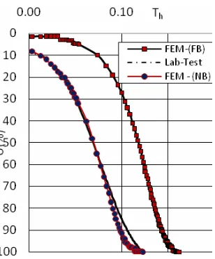
The Figures 21 and 22 are shown the relationship

be-tween case (NB) in FEM and lab test, the vacuum 50 kPa was applied only and combination to surcharge respec-tively. In the both cases the DOC in 100% were induced, the largest different of U is 3.5% between FEM and lab test occurring at Th = 0.3.

The final deformation of specimen nearly same value at end of vacuum stage and vacuum combine surcharge as shown in Figure 23. The largest different in volume

strain 0.3% occur at 350min as DOC at 95%.

The volume strain in 4.92% and 7.12% were found

both /e )

ted isotropic stress; this ratio is nearly one during vacuum only and re s a rch was estab he

The lts agre trong with behavi of

-provement by vacuum pre g theory.

T 24 is shown the increasing shea ren

of soil specim n be

pplica-tio a era gre

olida-t a 00% pe ly.

is shown in the Figure 25, there are

here

su/σv': determine with the lateral earth ratio K by the

conventional tri-axial test in Figure 18.

p: the loading is applied (vacuum pressure or surch- arge loading).

The undrain shear strength of soil specimen from lab test result is analysis to check the capacity of soil im- proved.

in cases FEM and Lab Test. The strain ratio (er v

illustrated the inward lateral deformation of specimen subjec

duce e s

s su ly

arge lis

soil d.

im

se resu or

loadin

he Figure r st gth

e n vacuum preloa

fore im ding provem t sev ent and l de after a e of cons ion of 40%, 70%

The stress path

Figure 21. Case n = 20, vacuum only; Va = 50 kPa, U = 100%.

Figure 22. Case n = 20, vacuum combine surchage; Va = 50 kPa, U = 100%.

Figure 24. Increasing undrained shear strength.

Figure25. Stress path.

some sections during simulate vacuum preloading me- thod, pre-consolidation (AB), vacuum application (BC), surcharge loading (CDEF). Under vacuum condition, the stress path of soil moves from B to C far from the failure line, while it changes from D to E close to the failure line when surcharge was applied. The behavior of soil speci-men under vacuum preloading method simulated by Tri-axial apparatus is well matched the before studies.

5. Conclusions

The study has been developed based on the combination of finite element analysis and the results of laboratory experiments to simulate a new appropriate method. This method can be widely applied for soft ground improve-ment by vacuum preloading method. The results om the

etric unit cell used to model the

behav-Figure 23. Case n = 20, vacuum combine surchage; Va = 50 kPa, U = 100%.

fr study can be summarized as follows:

ior of soil treatment by vacuum preloading as none boundary conditions are considered, the behavior of soil is more close to real soil state in the field.

2) Two cases of drainages boundary showed that time for consolidation in cases outside drainage of unit cell is faster than at the center by ThNC/ThNB ratio. However, the

deformations of the specimens in all cases are in same shape and value with the same applied condition.

3) Results of experiments by tri-axial apparatus en-tirely agree with FEM model. It is suggesting that the theories are given full compliance, highly compelling to predict the behavior of soil improvement by vacuum preloading method.

REFERENCES

[1]

mos-pheric Pressure,”

Stabilization, Massachusetts Institute of Technology, Bos-ton, 1952, pp. 258-263.

[2] B. Indraratna and I. W. Redana, “Laboratory Determina-tion of Smear Zone Due to Vertical Drain Installat

Journal of Geotechnical and Geoenvironmental

Engi-W. Kjellman, “Consolidation of Clayey Soils by At

Proceedings of a Conference on Soil

ion,”

neering, Vol. 124, No. 2, 1998, pp. 180-184. doi:10.1061/(ASCE)1090-0241(1998)124:2(180) [3] S. Hansbo, “Consolidation of Fine-Grained Soils by

Pre-. 1330- fabricated Drains,” Proceedings of 10th International Conference on Soil Mechanics and Foundation Engi-neering, Stockholm, Vol. 3, 1981, pp. 677-682.

[4] R. A. Barron, “Consolidation of Fine-Grained Soils by Drain Wells,” Transactions of ASCE, Vol. 113, 1948, pp. 718-742.

[5] B. Indraratna, C. Rujikiatkamjorn and I. Sathananthan, “Radial Consolidation of Clay Using Compressibility In-dices and Varying Horizontal Permeability,” Canadian Geotechnical Journal, Vol. 42, No. 5, 2005, pp 1341. doi:10.1139/t05-052

[6] J. C. Chai, J. P. Carter and S. Hayashi, “Vacuum Con-solidation and Its Combination with Embankment Load-ing,” Canadian Geotechnical Journal, Vol. 43, No. 10, 2006, pp. 985-996. doi:10.1139/t06-056