A Comparison of Various Normalization Methods for LC/MS Metabolomics Data

(1)

ISSN Online: 2156-8502 ISSN Print: 2156-8456

DOI: 10.4236/abb.2018.98022 Aug. 13, 2018 339 Advances in Bioscience and Biotechnology

A Comparison of Various Normalization

Methods for LC/MS Metabolomics Data

Jacob E. Wulff, Matthew W. Mitchell

Metabolon, Inc., Research Triangle Park, NC, USA

Abstract

In metabolomics data, like other -omics data, normalization is an important part of the data processing. The goal of normalization is to reduce the varia-tion from non-biological sources (such as instrument batch effects), while maintaining the biological variation. Many normalization techniques make adjustments to each sample. One common method is to adjust each sample

by its Total Ion Current (TIC), i.e. for each feature in the sample, divide its

intensity value by the total for the sample. Because many of the assumptions of these methods are dubious in metabolomics data sets, we compare these methods to two methods that make adjustments separately for each metabo-lite, rather than for each sample. These two methods are the following: 1) for each metabolite, divide its value by the median level in bridge samples (BRDG); 2) for each metabolite divide its value by the median across the ex-perimental samples (MED). These methods were assessed by comparing the correlation of the normalized values to the values from targeted assays for a subset of metabolites in a large human plasma data set. The BRDG and MED normalization techniques greatly outperformed the other methods, which of-ten performed worse than performing no normalization at all.

Keywords

Metabolomics, Normalization, Liquid Chromatography, Mass Spectrometry, TIC

1. Introduction

A major obstacle in global liquid chromatography mass spectrometry (LC-MS) based metabolomics is drawing comparisons between samples processed on dif-ferent runs of the same instrument or on difdif-ferent runs from difdif-ferent instru-ments. There are a number of reasons for wanting to compare samples from

dif-How to cite this paper: Wulff, J.E. and Mitchell, M.W. (2018) A Comparison of Various Normalization Methods for LC/MS Metabolomics Data. Advances in Bioscience and Biotechnology, 9, 339-351. https://doi.org/10.4236/abb.2018.98022

Received: June 14, 2018 Accepted: August 10, 2018 Published: August 13, 2018

(2)

DOI: 10.4236/abb.2018.98022 340 Advances in Bioscience and Biotechnology

ferent instrument runs. Single runs using a mass spectrometer are limited to a certain number of samples. When run through a mass spectrometer, samples are prepped and placed on a plate containing a defined number of wells with each well housing an individual sample. The number of wells available depends on the type and size of plate used, but is generally some multiple of 24 [1]. Even in-strumentation that can accommodate large plates or multiple small plates is generally restricted to, at most, a few hundred wells [2]. Large epidemiological studies with thousands of samples can easily surpass this capacity. In another example, a designed time course experiment may not have all samples available at one time for analysis. In particular, the clinical environment is analogous to these situations as new patients are regularly being admitted and evaluated. However, mass spectrometry itself is inherently semi-quantitative; the observed

value returned by the instrument is the ion count associated with the feature, i.e.

“ion peak”, which depends not just on the concentration in the sample but also on metabolite and instrument characteristics.

Exact concentration can be derived though calibration curves, i.e. standard

curves, in which known concentrations of the target metabolite are included as a way to orient the ion counts and estimate the levels in samples of interest ac-cording to their position on the curve. For a thorough review of standard curves

see the five part series by Dolan [3] [4] [5] [6] [7]. This targeted approach is

clearly infeasible for global metabolomic profiling as 1) the metabolites to be

captured are not known a priori 2) it is a significant challenge to obtain a labeled

standard for each metabolite and 3) there are a limited number of wells available to house the standards along with the experimental samples being profiled.

Lacking full quantitation, one must find some way to adjust the ion counts in different batches to each other. Batch effects are typically removed through normalization. The goal of normalization is to reduce the systematic variation but preserve the biological variation. Many normalization techniques used in the field adjust each sample. However, there are other normalization techniques that make adjustments for each metabolite, rather than the sample. Often normaliza-tion techniques are deemed successful if the variance has decreased. However, some of the important biological variation may have been removed also. Since the ideal measurement for a metabolite would be from a targeted assay or clini-cal measurement, we compare the normalized values to the values from a panel of targeted assays, where the concentrations have been measured.

2. Materials and Methods

2.1. Traditional Normalization

(3)

sus-DOI: 10.4236/abb.2018.98022 341 Advances in Bioscience and Biotechnology

ceptible to being overly influenced by a small number of features with very high ion observations. This normalization also assumes that most metabolites are not changing under the conditions being tested and that there are roughly equal numbers of metabolites that are both up and down-regulated. This assumption is clearly violated in some sample sets, such as comparisons between cell lines or when comparing normal tissue to cancerous tissues.

Various adjustments to this basic premise include median normalization, MS-total useful signal (MSTUS) [9], median absolute deviation (MAD) [10], probabilistic quotient normalization (PQN) [11] and cyclic locally weighted

re-gression (Cyclic LOWESS) [12] among others [13] [14]; however, in general,

these models rely on the assumption that on “average” the ion count of each sample should be more or less equal if there were no instrument batch effects. In this paper normalizations are separated into three classes depending on the me-chanism of action. The first class involves dividing ion intensities by a function of the sample’s spectra. The second class of normalization relies on Mi-nus-Average (MA) plots. The third class is those normalizers that do not fit into either of the first two classes.

2.1.1. Class I—Spectral Division

Normalizers of the first class are defined as being a ratio of the sample’s raw

in-tensity values and a function of the sample vector. Let Xi=

{

xi1xim

}

be the

vector of observed ion counts for metabolites 1,2, , , m for sample i, and let

N i

X represent the resulting vector of normalized metabolites. Normalizers of

the first class are defined as

( )

N i

i

i i X X

f X =

where ƒ ( )i • is some function. For example, for TIC ƒi is the sum of all the

raw peak areas in sample i, and thus N

i

X is a vector where the original values

have been scaled by this sum.

Table 1 summarizes ƒi for the first class of normalizations. Several are vari-ations on TIC, such as MS Total Useful Signal (MSTUS) which restricts to only those features that are common to all samples. Vector Normalization (VECT), takes TIC into two dimensions by measuring the Euclidean distance of the ob-served vector from the origin 0, and for this reason is sometimes referred to as “Euclidean Norm”. Both TIC and VECT are specific versions of the more

gener-al form p p

ij x

Σ _{. “Mean” is simply TIC adjusted for the number of features while}

“Median” used the median spectra from sample. Median Absolute Deviation (MAD) takes “Median” a step further by finding the absolute deviations from the median within a sample and using the median of these to normalize. Some methods normalize to a baseline or control spectrum. Such spectra can be

de-termined a priori or chosen from the available samples, such as the sample with

(4)

[image:4.595.210.539.86.268.2]

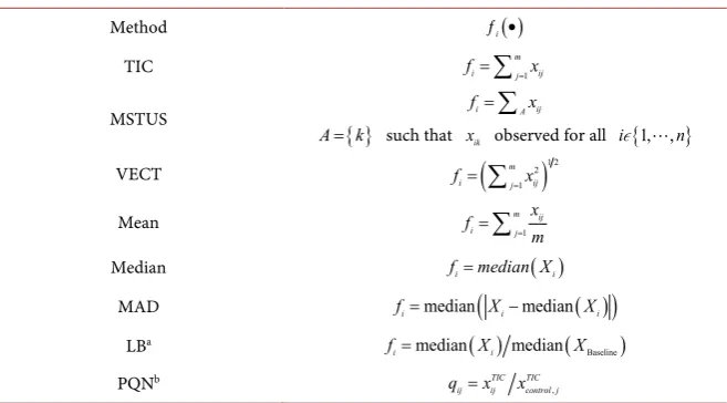
Table 1. Class I Normalizers.

Method ƒi( )•

TIC 1

m i j ij

f =

∑

₌x

MSTUS fi=

∑

Axij

{ }

A= k such that xik observed for all i{1, ,n}

VECT

(

2

)

1 2

1

m i j ij

f =

∑

=x

Mean m₁ ij

i j

x f

m

=

∑

Median f median Xi= ( )i

MAD fi=median

(

Xi−median

( )

Xi

)

LBa ( ) ( )

Baseline

median median

i i

f = X X

PQNb

,

TIC TIC ij ij control j

q =x x

a,b_{Baseline/Control spectrum may be taken from a designated sample or calculated from available data, such}

as sample with median TIC.

TIC of the resulting normalized sample is equal to that of the “baseline”. LB as-sumes a constant linear relationship between the sample and the baseline. Non-linear extensions are available. Although the name includes “scaling”, the intent is consistent with normalization which seeks to adjust all spectrum of each sample to the same level in some sense and the computation is consistent with the Class I definition. PQN, which involves a four-step process, is the most computation intensive of Class I normalizers listed here. In the first step TIC normalization is performed. Second, a control spectrum is calculated – this may be based upon a designated sample or the median spectra from all samples may

be used. Third, for each feature the ratio, i.e. quotient, of the TIC normalized

in-tensity of the sample and control spectrum is found. The final normalizer is then the median of all quotients. Most of the other class I normalizers are reasonably straightforward to calculate and are not time intensive from a computational standpoint. Hence, these are popular and common choices for normalizing.

2.1.2. Class II—MA Normalizers

The second class of normalizers involve MA plots, which are derived from

Alt-man-Bland plots on the log scale [15] [16]. For any two samples j and j′_the

MA plot is a scatter plot where each metabolite, i, has coordinates

(

minus ,ij avgij

)

given by

( )

2 2

minusij =log xij −log xij′

( )

2 2

log log

2

ij ij

ij

x x

avg = + ′ _.

(5)

the difference between the two samples due to the systematic variation. Under Cyclic LOWESS, a non-linear local regression curve (LOWESS) is fitted to the MA plot for a given pair of samples. The process is then repeated for all possible pairwise combinations of samples in the data set. Following a complete iteration over all samples, the cycle is repeated until some tolerance is achieved between the latest cycle and the preceding one.

Another variation on this is contrast normalization [17]. Under contrast

nor-malization the complete set of all ion features for all samples X =

[

X1Xn

]

′ is

log transformed and then linearly transformed using a k by k orthonormal

matrix M to produce a new set of orthogonal vectors:

( )

log

O

X = X M• _.

The first row of M is the repetition of the constant 1 k. The other rows

of M are not uniquely defined, except in the case of k=2 which gives

2 1 ₁ ₁

2 1 1 M −   = _ _  .

For k>2_, M is not unique, which requires some consideration for the

next step in which 0

1

X , the first row of _YO_{, is used to predict the remaining}

rows 0

i

X for i=2, , n . Referring to these predictions as ˆ0

i

X , using

LOWESS regression with weighted least squares produces ˆ0

i

X s′ that are

inva-riance to the choice of M. Estimation of ˆ0

i

X s′ is iterated until some tolerance

between the previous and newest estimate is achieved. The final normalized ma-trix is then given by

(

) (

)

N 0 0 0 0 0

1 2 ˆ2 m ˆm

X =_X X −X  X −X _′.

From this point the data set may be analyzed or mapped back to the original space via the reverse transformation

(

N

)

exp X •M .

The similarity to cyclic LOWESS may not be immediately obvious; however,

notice that when k=2 the contrast matrix M coupled with the log

trans-formation is analogous to the orientation of the MA plot. Contrast normaliza-tion essentially generalizes the MA concept to higher dimensions.

2.1.3. Class III—Other

Normalizations that do not fit the criteria of Class I or Class II are classified here. One example of this is Quantile Normalization (Quant) [18]. This method rescales so that the distribution of intensities within each sample is the same

across all samples. Let Xi be the ordered set of intensities for sample

i

:

{

[1] [ ]

}

i i i m

X = x x ,

and consider the vector of average ordered statistics across all Xi

{

}

1 [1] 1 [ ]

[1] [ ]

n n

i i m

i i

m

x x

X x x

(6)

This essentially orders each row of the data set and then takes the average of each column. The normalized vector for a sample is then replaced with these values in the order corresponding to the ranks of un-normalized vector:

( ) ( )

{

1

}

N

i im

i rank x rank x

X = x__ ___x__ __ _.

An advantage to Quant is that it directly puts the intensities of each sample on the same scale, making sample to sample comparisons easier. One drawback is that features with missing values must be removed or imputed. Second, metabo-lites that are significantly more abundant may be normalized to a near static state. In fact, in the data set used in 2.4, oleic acid had the highest peak areas in every sample, so all of its values would all normalize to the same value. The same issue could apply to metabolites that are significantly lower in abundance than all other metabolites because metabolites near the limit of detection often drop out, i.e., no peak is detected.

2.2. Bridge Normalization (BRDG)

Mass spectrometry returns an ion count that is proportional to the true concen-tration but also dependent on the instrumentation. Rocke and Lorenzato [19] proposed a model for this ion count meant to account for the different perfor-mance behavior observed at low and high concentrations. Using this model,

consider two separate instrument runs in which k technical replicates of the

same sample are run in both batches. The ion intensity of the ith_{metabolite in}

batch b

{ }

1,2 for any replicate j

{

1, , k

}

is given as

eijb .

ijb ib i ijb x =β y η +ε

The subscript of the sample concentration, yi, is dependent only on the

bio-chemical since the k samples are technical replicates. βib relates to the

ioniza-tion effeciency of the instrument, and will vary by metabolite and batch.

(

_0, 2

)

ib N ηib

η ∼ σ and

(

_0, 2

)

ib N εib

ε ∼ σ are both normal, random errors with the

former dominating at higher concentrations and latter dominating at lower concentrations. Note that the intercept term, which is related to the background level of the instrument, has been removed, as it is generally regarded as a nuis-ance parameter and is in fact ignored in single point calibration curves [20]. The expected value of any such replicate is then:

2 ₂

e ib .

ib ijb ib i

µ ₌E x_ _₌_β y ση  

Shuffling the order of these terms gives

(

2 ₂

)

e ib .

ib ijb ib i

µ ₌E x_ _₌ _β ση y

 

As both βib and

2 ₂

eσηib _{are fixed, but unknown, parameters depending only}

on the metabolite and batch, these terms may be combined into a single

un-known variable. Letting e 2ib2

ib ib ση

β∗ ₌β _{it is easy to see that mean ion count for}

(7)

DOI: 10.4236/abb.2018.98022 345 Advances in Bioscience and Biotechnology *

ib ib i µ =β y

Hence, the mean ion count for the two batches is proportional:

1 2

i i

µ µ

β∗ =β∗

By the law of large numbers, there exists a k such that average of the replicates

within a batch

1

e jib

k

ib i jib

ib j

y k x

η

β ε

=

+ =

∑

is reasonably close to βib i∗y. Scaling each batch against the mean of these

repli-cates would thus eliminate the batch differences.

Data processing often includes QC samples as part of the metabolomic workflow in order to monitor instrument performance [21] [22]. These samples are aliquots of a pooled material and can be regarded as technical replicates and provide a convenient source for estimating the scaling factor. These samples will hence forth be referred to as bridge samples. To perform bridge sample norma-lization (BRDG), for each metabolite in a given instrument batch, divide its val-ues by the median of the bridge samples for that batch. The median rather than the mean is recommended in order to mitigate the influence of outliers.

2.3. Median Run Normalization (MED)

An important part of the experimental protocol should be randomization of the samples across the instrument runs. Under such randomization, for a given me-tabolite, the expected value of the relative concentration is the same for each in-strument run if there were no batch effects. Hence, randomly assigning the sam-ples and dividing the values for each metabolite on each instrument run day by the observed median should put each batch on the same scale. This is similar to the bridge normalization only with the samples themselves serving as the bridging.

Theoretically, the sample mean is generally a more consistent estimator than the sample median, but in skewed distributions and low sample sizes the effi-ciency of the mean can be impaired. Due to the propensity for extreme outliers in metabolomic data, which could adversely affect the sample mean, the median is used instead. This normalization procedure will be referred to as “MED”, henceforth.

2.4. Human Plasma Data Set

(8)

Plasma samples were obtained from participants in the Insulin Resistance Atherosclerosis Family Study (IRASFS), which was sponsored by the National Heart, Lung and Blood Institute with the goal of examining the genetic

epidemi-ology of insulin resistance and visceral adiposity [23]. The IRASFS consists of

subjects from Hispanic and African American families. From this cohort, 1719 samples were sent to Metabolon for global LC-MS metabolomic profiling – for

further details on this platform see Long et al. [24]. One sample was blank and

two other samples were duplicates, so these were removed. Thus, 1716 samples were used for analysis. Accommodating this many samples required between 13 and 15 instrument runs per arm of the platform. The resulting analysis meas-ured 1274 metabolites (922 named, 352 unnamed).

Plasma samples from these participants were also run on a separate targeted assay of seven metabolites, which were shown to be markers for impaired glu-cose tolerance (IGT) [25]. The metabolites measured in this panel are 2-hydroxybutyrate, 3-hydroxybutrate, 4-methyl-2-oxopentanoate, linoleoyl-GPC, oleic acid, pantothenic acid and serine. Additionally, a targeted sterol panel was run [26]. This panel contained two metabolites that were also present on the un-targeted platform: alpha-tocopherol and cholesterol. The bridge samples used were technical replicates of a pool of human plasma obtained from Bioreclama-tion.

Resulting normalized levels of these nine metabolites in the global panel are

compared to the targeted results using Pearson’s correlation, r. All analysis was

performed in R version 3.4.3 [27]. The following packages were used: limma

package [28] and Data Normalization R-script by Hochrein et al. [29].

3. Results and Discussion

For a preliminary analysis, a variance components analysis was performed for the bridge samples in order to assess how much of the variation can be attri-buted to the instrument batch. Those metabolites present in at least 80% of the bridge samples were used for this analysis (1049 metabolites). The variance components were fitted with JMP v13 [30]. From this analysis, one can obtain the percent of the variance that can be explained by the instrument batch. The

median batch variance component is 85%, i.e., for a typical metabolite, the

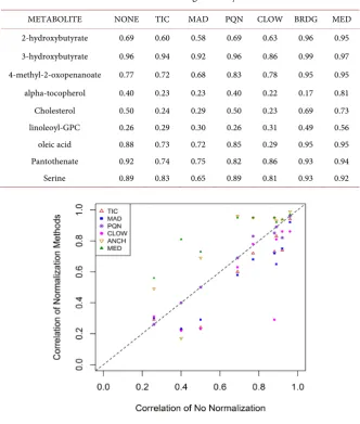
va-riance from the batch is 85% of the total vava-riance. For the metabolites compared to the targeted assays, their batch variance components are shown in Table 2.

The correlations of the normalized data to the targeted assays are shown in Table 3. This is graphically displayed in Figure 1. In Figure 1, those metabolites above the line y = x have correlations better than no transformation, while those

below have worse correlations. “NONE” refers to no normalization, i.e., the raw

(9)

[image:9.595.203.539.88.260.2]

Table 2. Variance Components for BATCH.

METABOLITE % Var from BATCH

2-hydroxybutyrate 96

3-hydroxybutyrate 85

4-methyl-2-oxopentanoate 95

alpha-tocopherol 89

cholesterol 84

linoleoyl-GPC 74

oleic acid 85

pantothenic acid 72

[image:9.595.206.539.285.677.2]

serine 70

Table 3. Correlation of normalized values to targeted assays.

METABOLITE NONE TIC MAD PQN CLOW BRDG MED

2-hydroxybutyrate 0.69 0.60 0.58 0.69 0.63 0.96 0.95 3-hydroxybutyrate 0.96 0.94 0.92 0.96 0.86 0.99 0.97 4-methyl-2-oxopenanoate 0.77 0.72 0.68 0.83 0.78 0.95 0.95 alpha-tocopherol 0.40 0.23 0.23 0.40 0.22 0.17 0.81

Cholesterol 0.50 0.24 0.29 0.50 0.23 0.69 0.73

linoleoyl-GPC 0.26 0.29 0.30 0.26 0.31 0.49 0.56

oleic acid 0.88 0.73 0.72 0.85 0.29 0.95 0.95

Pantothenate 0.92 0.74 0.75 0.82 0.86 0.93 0.94

Serine 0.89 0.83 0.65 0.89 0.81 0.93 0.92

Figure 1. Comparisons of Correlations to the Targeted Assays.

[image:9.595.206.539.294.675.2]

(10)

[image:10.595.206.538.68.379.2]

Figure 2. Comparison of normalized values for 2-hydroxybutryate. Colors represent

in-dividual batches. The values on the y-axis are the normalized values (except “Raw” which are the unnormalized values).

even greater than 0.9. From Table 3 and Figure 1, one can see that in general, the normalization methods that rely on metabolite-specific adjustments (BRDG, MED) significantly outperform the methods that make adjustments across each sample (TIC, MAD, PQN, CLOW). In fact, for many cases the sample-based normalizations performed worse than performing no normalization. For BRDG and MED, many of the resulting correlations are over 0.9. In general, BRDG and MED have similar performance, except for alpha-tocopherol. For al-pha-tocopherol, there were two batches that had a significant drop in peak areas for the bridge samples, but not for the experimental samples. Without these two batches, the correlation is 0.79. The bridge samples were obtained from a differ-ent source than the experimdiffer-ental samples. In general, it is preferable to run bridge samples from the same source as the experimental samples, as the quan-titation of metabolites can be affected by other substances within the sample.

4. Conclusion

(11)

sam-DOI: 10.4236/abb.2018.98022 349 Advances in Bioscience and Biotechnology

ples are known. Many common normalization techniques that make corrections across each sample, such as TIC normalization, often performed worse than performing no normalization at all. The two methods that relied on metabo-lite-specific correlations (BRDG, MED) performed much better than the sam-ple-based normalizations, and many of the resulting correlations were over 0.9. Correcting by the median batch value from the experimental samples (MED) can work well in a variety of applications. However, if one wants to run a very small set and merge into previous data sets or compare the values in two differ-ent data sets, it is probably better to normalize by bridge samples (BRDG). The main drawback of BRDG is that metabolites that are not present in the bridge samples cannot be normalized. Additionally, if the bridge samples are obtained from a different source, there may be some metabolites that have different batch effects in the bridge samples than in the experimental samples. To avoid this is-sue, having the bridge samples as similar as possible to the experimental samples is recommended.

Acknowledgements

The IRASFS was supported by the National Institutes of Health (HL060944, HL061019, HL060919, and DK085175).

Conflicts of Interest

The authors declare no conflicts of interest regarding the publication of this pa-per.

References

[1] Thermo Fisher Scientific (2017) Thermo Scientific Plastics Consumables. https://www.thermofisher.com/us/en/home/brands/thermo-scientific/molecular-bi ology/thermo-scientific-plastics-consumables.html

[2] Tachibana, C. (2014) What’s Next in ’Omics: The Metabolome. Science, 345, 1519-1521. https://doi.org/10.1126/science.345.6203.1519

[3] Dolan, J.W. (2009) Calibration Curves Part I: To b or Not to b? Chromatography Online, 27, 224-230.

[4] Dolan, J.W. (2009) Calibration Curves Part II: What Are the Limits? Chromatogra-phy Online, 27, 306-312.

[5] Dolan, J.W. (2009) Calibration Curves Part III: A Different View. Chromatography Online, 27, 392-400.

[6] Dolan, J.W. (2009) Calibration Curves Part IV: Choosing the Appropriate Model.

Chromatography Online, 27, 472-479.

[7] Dolan, J.W. (2009) Calibration Curves Part V: Curve Weighting. Chromatography Online, 27, 534-540.

[8] Deininger, S.O., et al. (2011) Normalization in MALDI-TOF Imaging Datasets of Proteins: Practical Considerations. Analytical and Bioanalytical Chemistry, 401, 167-181. https://doi.org/10.1007/s00216-011-4929-z

(12)

Bio-DOI: 10.4236/abb.2018.98022 350 Advances in Bioscience and Biotechnology

medical and Life Sciences, 877, 547-552. https://doi.org/10.1016/j.jchromb.2009.01.007

[10] Webb-Robertson, B.J., Matzke, M.M., Jacobs, J.M., Pounds, J.G. and Waters, K.M. (2011) A Statistical Selection Strategy for Normalization Procedures in LC-MS Pro-teomics Experiments through Dataset-Dependent Ranking of Normalization Scal-ing Factors. Proteomics, 11, 4736-4741. https://doi.org/10.1002/pmic.201100078 [11] Dieterle, F., Ross, A., Schlotterbeck, G. and Senn, H. (2006) Probabilistic Quotient

Normalization as Robust Method to Account for Dilution of Complex Biological Mixtures. Application in 1H NMR Metabonomics. Analytical Chemistry, 78, 4281-4290. https://doi.org/10.1021/ac051632c

[12] Yang, Y.H., et al. (2002) Normalization for cDNA Microarray Data: A Robust Composite Method Addressing Single and Multiple Slide Systematic Variation.

Nucleic Acids Research, 30, e15. https://doi.org/10.1093/nar/30.4.e15

[13] Sysi-Aho, M., Katajamaa, M., Yetukuri, L. and Oresic, M. (2007) Normalization Method for Metabolomics Data Using Optimal Selection of Multiple Internal Stan-dards. BMC Bioinformatics, 8, 93. https://doi.org/10.1186/1471-2105-8-93

[14] Nezami Ranjbar, M.R., Zhao, Y., Tadesse, M.G., Wang, Y. and Ressom, H.W. (2013) Gaussian Process Regression Model for Normalization of LC-MS Data Using Scan-Level Information. Proteome Science, 11, S13.

https://doi.org/10.1186/1477-5956-11-S1-S13

[15] Altman, D.G. and Bland, J.M. (1983) Measurement in Medicine: The Analysis of Method Comparison Studies. The Statistician, 32, 307-317.

https://doi.org/10.2307/2987937

[16] Bland, J.M. and Altman, D.G. (1986) Statistical Methods for Assessing Agreement between Two Methods of Clinical Measurement. The Lancet,1, 307-310.

https://doi.org/10.1016/S0140-6736(86)90837-8

[17] Astrand, M. (2003) Contrast Normalization of Oligonucleotide Arrays. Journal of

Computational Biology,10, 95-102.https://doi.org/10.1089/106652703763255697

[18] Bolstad, B.M., Irazarry, R.A., Astrand, M.T. and Speed, P. (2003) A Comparison of Normalization Methods for High Density Oligonucleotide Array Data Based on Va-riance and Bias. Bioinformatics,19, 185-193.

https://doi.org/10.1093/bioinformatics/19.2.185

[19] Rocke, D.M. and Lorenzato, S. (1995) A Two-Component Model for Measurement Error in Analytical Chemistry. Technometrics, 37, 176-184.

https://doi.org/10.1080/00401706.1995.10484302

[20] Peters, F.T. and Maurer, H.H. (2007) Systematic Comparison of Bias and Precision Data Obtained with Multiple-Point and One-Point Calibration in Six Validated Multianalyte Assays for Quantification of Drugs in Human Plasma. Analytical

Chemistry,79, 4967-4976.https://doi.org/10.1021/ac070054s

[21] Kenny,L.C., et al. (2010) Robust Early Pregnancy Prediction of Later Preeclampsia Using Metabolomic Biomarkers. Hypertension,56, 741-749.

https://doi.org/10.1161/HYPERTENSIONAHA.110.157297

[22] Zhou, B., Xiao, J.F., Tuli, L. and Ressom, H.W. (2012) LC-MS-Based Metabolomics.

Molecular BioSystems, 8, 470-481.https://doi.org/10.1039/C1MB05350G

[23] Henkin, et al. (2003) Genetic Epidemiology of Insulin Resistance and Visceral Adi-posity. The IRAS Family Study Design and Methods. Annals of Epidemiology, 13, 211-217. https://doi.org/10.1016/S1047-2797(02)00412-X

(13)

Va-DOI: 10.4236/abb.2018.98022 351 Advances in Bioscience and Biotechnology

riants Associated with Human Blood Metabolites. Nature Genetics, 49, 568-578.

https://doi.org/10.1038/ng.3809

[25] Cobb,J., et al. (2015) A Novel Test for IGT Utilizing Metabolite Markers of Glucose Tolerance. Journal of Diabetes Science and Technology,9, 69-76.

https://doi.org/10.1177/1932296814553622

[26] Kaddurah-Daouk, R., et al. (2011) Enteric Microbiome Metabolites Correlate with Response to Simvastatin Treatment. PLoS ONE,6, e25482.

https://doi.org/10.1371/journal.pone.0025482

[27] R Core Team (2017) R: A Language and Environment for Statistical Computing. R Foundation for Statistical Computing, Vienna. https://www.R-project.org/

[28] Ritchie, M.E., et al. (2015) Limma Powers Differential Expression Analyses for RNA-Sequencing and Microarray Studies. Nucleic Acids Research, 43, e47.

https://doi.org/10.1093/nar/gkv007

[29] Hochrein, J., et al. (2015) Data Normalization of (1)H NMR Metabolite Finger-printing Data Sets in the Presence of Unbalanced Metabolite Regulation. Journal of

Proteome Research,14, 3217-3228.https://doi.org/10.1021/acs.jproteome.5b00192