—AG1 approximation method of conic sections

(1)

G

1 Approximation of Conic Sections by

Bernstein-Jacobi Hybrid Polynomial Curves

Mao Shi

Abstract—A G1 approximation method of conic sections using Bernstein-Jacobi hybrid polynomial curves of arbitrary degree is proposed. Based on the method of weighted-sum-of-objective-function in the multi-objective optimization, the prob-lem can be converted to a scale optimization. Applying weighted least-squares, we obtain the resulting curve. Meanwhile, by the orthogonality of Jacobi polynomials, the inverse of matrix is avoided. Finally, some examples and figures were offered to demonstrate the efficiency and the simplicity of our methods.

Index Terms—Conic sections, Geometric continuity, Hybrid curves, Multi-objective optimization, Least-squares

I. INTRODUCTION

A

LTHOUGH rational Bézier curves are the standard in the Initial Graphics Exchange Specification (IGES), some Computer Aided Design (CAD) systems only use polynomial expressions to deal with parametric curves. This is because rational Bézier curves can’t be differentiated and integrated easily [1]–[6]. Many research papers have been published about approximation of conic sections by Bézier curves since 1980s. Using geometric information such as point positions, tangents and curvatures, De Boor et al. [7] first applied Geometric Hermite Interpolation (GHI) method to accomplish a high accuracy approximation of circular arcs based on cubic Bézier curves. Floater [8] [9] studied approximation by quadratic splines and Bézier curves of odd degree n respectively. Both methods have the optimal approximation order2n. Fang [10] presented methods for ap-proximating conic sections using quintic polynomial curves. The constructed quintic polynomial curve hasG3_-continuity with the conic section at the end points and G1_-continuity at the parametric mid-point. Using the matrix form and the least squares method, Hu [11] researchedG1 _{approximation} of conic sections by Bézier curves of arbitrary degree inL2 norm, but the method requires to compute matrix inversion. In this paper, we mainly interested in theG1 approxima-tion of conic secapproxima-tions by Bézier curves of arbitrary degree. In order to avoid calculating the inverse of matrix in L2 _norm, we construct a Jacobi-Berenstein hybrid polynomial curve. With the help of the weighted sum method in multi-objective optimization [12] [13] [14] and the weighted least squares method we obtain results.

The rest of the paper is organized as follow. In Section 2, some basic definitions and properties on conic sections and Jacobi-Bernstein polynomial curves were given. The problem of G1-constrained approximation of the conic sections is

Manuscript received October 22, 2018; revised January 22, 2019. This work is supported by the Fundamental Research Funds for the Central Universities (GK201703007).

Mao Shi is with the School of Mathematics and Information Sci-ence of Shaanxi Normal University, Xi’an 710062, China. e-mail: [email protected]

described. In Section 3, using the weighted least-squares method we introduce an explicit algorithm to solve the problem. Approximation errors and numerical examples are presented in Section 4 to confirm the effectiveness of the method. Finally, in Section 5 we conclude this paper.

II. PRELIMINARIES

A conic section can be represented in the standard rational B´ezier form by

P(t) = c(t)

ω(t)

=B

2

0(t)p0+B 2

1(t)ω1p1+B 2 2(t)p2

B2

0(t)+B12(t)ω1+B22(t)

, t∈[0,1], (1)

whereω1∈R+ is the weight,pi = (xi, yi) are the control

points and Bn i(t) =

n i

ti₍₁ ₋_t₎n−i _{are the Bernstein}

polynomials.

A Jacobi-Bernstein hybrid curveQ˜(t)of degreencan be expressed as

˜

Q(t) =

r

X

i=0

qiBin(t) +ϕ(t)

N

X

j=0

˜

qjJ_j(r+1,s+1)(u)

+ n

X

i=n−s

qiBin(t), (2)

whereN =n−(r+s+2),u= 2t−1,ϕ(t) =tr+1₍₁₋_t₎s+1_,

qi = (¯xi,y¯i) are the control points of the B´ezier curves,

˜

qi= (˜xi,y˜i)are the control points of the Jacobi curves and

J_j(r+1,s+1)(u)are the Jacobi polynomials.

Setρ(t)>0is a weight function and Fx _and_Fy _{are the}

components of the vector equation

(Fx, Fy) =

Z 1 0

ρ(t)P(t)−_Q˜₍_t₎2_dt.

Based on the method of weighted-sum-of-objective-function, the problem ofG1 _{approximation of the conic section}_P₍_t₎ by B´ezier curves is to find a Jacobi-Bernstein hybrid curve

˜

Q(t)of degreenso that

Fλ, η,{q˜i}n

−(r+s+2)

i=0

= 1 2(F

x

+Fy), (3)

is minimized and the control points at the end points satisfy

q0 =p0, qn=p2,

q₁=p₀+2ω

n λ∆p0, qn−1=p2−

2ω

n η∆p1, (4) whereλandη are free parameters.

Next, we review and derive several of mathematical pre-liminaries on Bernstein polynomials, classical Jacobi poly-nomials and conic sections which are used in the paper.

Lemma 1.Setting Bnj

ij (t) be a Bernstein polynomial of

degreenj, multiplication ofmBernstein polynomials satisfy

IAENG International Journal of Applied Mathematics, 49:2, IJAM_49_2_08

(2)

the following equation [6],

m

Y

j=1

Bnj ij (t) =

M N J

B

N

J(t), (5)

and the corresponding definite integral can be written as Z1

0

m

Y

j=1

Bnj ij(t)dt=

M

(N+ 1) N_J, (6)

whereM =Qm_j₌₁ nj

ij

,N =Pm_j₌₁nj andJ =Pm_j₌₁ij. Lemma 2.Given two B´ezier curvesX(t) =

n P

j=0

xn_jB_jn(t)

of degreenandY(t) = m P

k=0

ym_k B_km(t)of degreem, we have [15]

X(t)Y(t) =

m+n

X

i=0

Ci(ymk,x n j)B

m+n

i (t), (7)

where

Ci(ymk,x n j) =

min(m,i) X

l=max(0,i−n)

m l

n i−l

m+n i

y

m l x

n

i−l. (8)

Lemma 3. A Jacobi polynomial can be represented by Bernstein polynomials as follows [16]

J_j(r+1,s+1)(u) = j X

i=0

aj_iB_ij(t), (9) where

aj_i := (−1)(i+j) j+r+1

i

j+s+1

j−i

j i

. (10)

Furthermore, using (7), (9) and (10), we obtain

¯

Gα,βi,j (α, β, i, j)

=

Z1 0

tα(1−t)βJ_i(r+1,s+1)(u)J_j(r+1,s+1)(u)dt

=

Z1 0

Bαα(t)B β

0(t)

i

X

m=0

aimB i m(t)

j

X

l=0

aj_lB_lj(t)dt

= i+j

X

l=0

Cl(aim, a j l)

Z 1 0

Bαα(t)B β

0(t)B

i+j l (t)dt

= 1

α+β+i+j+ 1 i+j

X

l=0

i+j l

α+β+i+j α+l

Cl(a

i

m, aj_l), (11)

whereCl(aim, a j

l)are scale forms of (8).

Moreover, when α=s+ 1andβ =r+ 1, the equation

¯

Gα,β_i,j (α, β, i, j)has the orthogonality, that is

γ_i(s+1,r+1)= ¯Gα,β_i,j (s+ 1, r+ 1, i, j) =

 

 1 2i+r+s+3

(i+s+1

s+1 )

(i+r+s+2

s+1 )

i=j,

0 i6=j. (12)

Similarly, given a Jacobi polynomialJ_j(r+1,s+1)(u)and a Bernstein polynomialB_kn(t), we have

Gα,β_i,j (α, β, k, j) =

Z1 0

tα(1−t)βBkn(t)J

(r+1,s+1)

j (u)dt

= 1

α+β+n+j+ 1 j

X

i=0

(−1)(i+j) n k

j+r+1

i

j+s+1

j−i

α+β+n+j α+k+i

. (13)

Lemma 4.LetX(t) = n P

i=0

xn

iBin(t)be a B´ezier curve of

degreenandP(t)be a conic section given by equation (1), we have

ξ(n,xni) =

Z1 0

X(t)P(t)dt

= n+2 X

i=2

i−1 X

s=1

n+ 2 i

!

aas∆i_cn+2 0

i−s +aA

×        4 √

4a−1arctan 1 √

4a−1, a > 1 4, 2

√ 1−4aln

1−√1−4a

1+√1−4a

, a <

1 4,

−4, a= 1₄,

(14)

where a=₂₍₁₋1_ω

1), ai= 2−(i−1)

[(i−1)/2]

P

s=0

i

2s+1

(1−4a)s_{, i}

6n+ 2, an+3= 2−(n−2)a

[n/2]

P

s=0

n−1 2s+1

(1−4a)s, and

A=cn0+2+

(n+2)∆cn₀+2

2 +

an+2 2 +an+3

nP+2

i=2

n+2

i

∆icn0+2. Finally, for a Jacobi polynomialJ_j(r+1,s+1)(u)and a conic sectionP(t), by (14), it yields

ξ(r+s+j+ 2, ck)

=

Z 1 0

tr+1(1−t)s+1J_j(r+1,s+1)(u)P(t)dt

=

Z 1 0

P(t)

j

X

i=0

(−1)(i+j) j+r+1

i

j+s+1

j−i

r+s+j+2

r+i+1 B

r+s+j+2

r+i+1 (t)dt

=

Z 1 0

P(t)

r+j+1 X

k=r+1

ckBr_k+s+j+2(t)dt

=

Z 1 0

P(t)

r+s+j+2 X

k=0

ckB_kr+s+j+2(t)dt

where

ck=

 



(−1)(k−r−1+j)( j+r+1

k−r−1)(

j+s+1

j−k+r+1)

(r+s+j+2

k )

, k=r+1, ..., r+j+1,

0, others.

III. G1

POLYNOMIAL APPROXIMATION OF CONIC SECTIONS

The G1 approximation of conic sections means r=s= 1. According to the method of weighted least squares [16], derivatives ofF(·)with respective to pointsq˜k must be zero,

so we have Z 1

0

ρ(t)ϕ(t)P(t)−Q˜(t)J_k(2,2)(2t−1)dt= 0.

Lettingρ(t) = 1

ϕ(t) and substituting (3), (12) and (13) into the above equation, we obtain

˜

qk=

1

γ_k(2,2)

( Z 1

0 "

P(t)−

1 X

i=0

Bni(t)p0+

n

X

i=n−1

Bin(t)p2 !

−2ω n (λB

n

1(t)∆p0−ηBnn−1(t)∆p1)

J_k(2,2)(u)dt

= 1

γ_k(2,2)

"

ξ(k, aki)−

1 X

i=0

p0G0i,k,0− n

X

i=n−1

p2G0i,k,0

−2ω

n λ∆p0G

0,0

1,k−η∆p1G

0,0

n−1,k

.

IAENG International Journal of Applied Mathematics, 49:2, IJAM_49_2_08

(3)

Setting

Ak=

1

γ_k(2,2)

"

ξ(k, aki)−

1 X

i=0

p0G0_i,k,0−

n

X

i=n−1

p2G0_i,k,0 #

,

Bk=

2ω∆p0G0₁,_,k0

nγ_k(2,2) and Ck=

2ω∆p1G0_n−,0₁_,k nγ_k(2,2) ,

˜

qk can be rewritten as

˜

qk =Ak−λBk+ηCk. (15)

From now on, we can calculate all the control points of the approximation curve Q˜(t)by equation (15). In order to obtain the values of λ andη, we substituting (15) into the objective function (3) and letting ρ(t) = 1 yield

(∂Fx ∂λ +

∂Fy ∂λ = 0 ∂Fx

∂η + ∂Fy

∂η = 0

(16)

and

∂(Fx, Fy)

∂λ =λΠ1−ηΠ2−Π3, ∂(Fx, Fy)

∂η =λΠ4−ηΠ5−Π6,

where

Π1=

Z 1 0

2ω n ∆p0B

n

1(t)−ϕ(t)

n−4 X

j=0

BjJ_j(2,2)(u)

!2

dt

=(2ω∆p0)

2

n(4n2₋₁₎−

4ω∆p0

n n−4 X

j=0

BjG21,,j2+ n−4 X

j=0

n−4 X

k=0

BjBkG¯4j,k,4,

Π2=Π4

=

Z 1 0

2ω n ∆p1B

n

n−1(t)−φ(t)

n−4 X

j=0

CjJ_j(2,2)(u)

!

× 2ω n ∆p0B

n

1(t)−φ(t)

n−4 X

j=0

BjJ_j(2,2)(u)

!

dt

=(2ω)

2

∆p0∆p1

(2n+ 1) 2_nn +

n−4 X

j=0

n−4 X

k=0

CjBkG¯4j,k,4

−2ω n

n−4 X

j=0

∆p0CjG21,,j2+ ∆p1BjG2n,−21,j

,

Π3=

Z 1 0

2ω n ∆p0B

n

1(t)−φ(t)

n−4 X

j=0

BjJ_j(2,2)(u)

!

× P(t)−

1 X

i=0

Bni(t)p0−

n

X

i=n−1

Bin(t)p2

−ϕ(t) n−4 X

j=0

AjJj(2,2)(u)

!

dt

=2ω∆p0 n

"

ξ(n, uλi)− n 2n+ 1

1 X i=0 n i p0 2n i+1 + n X

i=n−1

n i p2 2n i+1 ! − n−4 X

j=0

AjG21,,j2

#

− n−4 X

j=0

Bj ξ(j+ 4, ck)−

1 X

i=0

p0G2i,j,2

− n

X

i=n−1

p2G2i,j,2− n−4 X

i=0

AiG¯4i,j,4

!

,

Π5=

Z 1 0

2ω n ∆p1B

n

n−1(t)−ϕ(t)

n−4 X

j=0

CjJ_j(2,2)(u)

!2

dt

=(2ω∆p1)

2

n(4n2₋₁₎−

4ω∆p1

n n−4 X

j=0

CjG2n,−21,j+ n−4 X

j=0

n−4 X

k=0

CjCkG¯4_j,k,4

and

Π6=

Z 1 0

P(t)−

1 X

i=0

p0Bin(t)−

n

X

i=n−1

p2Bin(t)

−φ(t) n−4 X

j=0

CjJ_j(2,2)(u)

!

×

2ω n ∆p1B

n n−1(t)

−φ(t) n−4 X

j=0

CjJ_j(2,2)(u)

!

dt

=2ω∆p1

n ×[ξ(n, u η i)−

n (2n+ 1)

1 X i=0 n i p0 2n n+i−1

+ n

X

i=n−1

n i

p2

2n n+i−1

!

− n−4 X

j=0

AjG2_n,−21,j

#

− n−4 X

j=0

Cj ξ(j+ 4, ck)−

1 X

i=0

p0G2i,j,2

−

1 X

i=0

p2G2i,j,2− n−4 X

k=0

AkG¯4_j,k,4

!

,

where

uλi =

(

1 i=1

0 Others

and

uηi =

(

1 i=n-1

0 Others .

Finally, we can obtain control points˜q_iof equation (2) from the system of linear equations (16).

IV. NUMERICAL EXAMPLES

In this section, we provide two examples to show the effective of our method. For each example, we use discrete Hausdorff distances to express approximation error.

Example 1 (Also Example 1. in [11]) Given a conic sectionP(t)with control points(0,0),(1.2,1.5),(1,0) and the weight ω1 = 3. Table I lists λ,η and error obtained by Hu’s method and ours method, respectively. The resulting curves of degree n = 4 are shown in the left-hand side of Fig. 1 and the corresponding error distance curves are illustrated in the right-hand side of Fig. 1. Fig. 2 shows the resulting curves with degreen= 6 and corresponding error distance curves.

TABLE I

APPROXIMATION OF CONIC SECTIONS WITH POLYNOMIALS OF DEGREE

4AND6

n Hu’s method Our method

λ η ε λ η ε

4 0.8091 0.8273 2.14×10−2 0.8168 0.8368 1.94×10−2

6 0.9438 0.9507 5.1×10−3 0.9503 0.9524 5.1×10−3

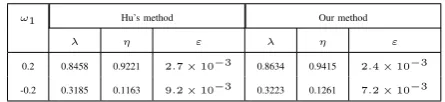
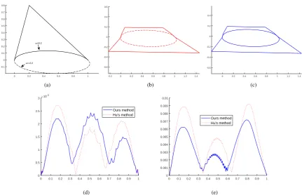
[image:3.595.299.508.51.363.2]

Example 2 (Also Example 2. in [11]) Given a conic sectionP(t)with control points(0,0),(0.2,0.8),(1,0) and the weight ω1 = 0.2 and ω1 = −0.2, respectively. Table II lists λ, η and error obtained by Hu’s method and ours method, respectively. The resulting curves are shown in (a) of Fig. 3 , the corresponding error distance curves forω1= 0.2 are illustrated in (b) of Fig. 3 and the corresponding error distance curves forω1= 0.2 are illustrated in (c) of Fig. 3.

IAENG International Journal of Applied Mathematics, 49:2, IJAM_49_2_08

(4)

-0.2 0 0.2 0.4 0.6 0.8 1 1.2 1.4 0

0.5 1 1.5

(a)

0 0.5 1 1.5

0 0.2 0.4 0.6 0.8 1 1.2 1.4 1.6 1.8

(b)

0 0.5 1 1.5

0 0.2 0.4 0.6 0.8 1 1.2 1.4 1.6 1.8

(c)

0 0.1 0.2 0.3 0.4 0.5 0.6 0.7 0.8 0.9 1

0 0.005 0.01 0.015 0.02 0.025

Ours method Hu's method

[image:4.595.57.280.641.692.2]

(d)

Fig. 1. (a) The conic section. (b) The resulting curve of degree 4 using Hu’s method. (c) The resulting curve of degree 4 using ours method (d) The

corresponding error distance curves. (For interpretation of the references to color in this figure legend, the reader is referred to the web version of this article.)

TABLE II

APPROXIMATION OF CONIC SECTIONS WITH POLYNOMIALS OF DEGREE

5

ω1 Hu’s method Our method

λ η ε λ η ε

0.2 0.8458 0.9221 2.7×10−3 0.8634 0.9415 2.4×10−3

-0.2 0.3185 0.1163 9.2×10−3 0.3223 0.1261 7.2×10−3

V. CONCLUSION

In this paper, we have studied G1-constrained approx-imation of conic section with arbitrary degree Bernstein-Jacobi hybrid polynomial curves. As [11] explained our method is to minimize the L2-error distance rather than to

minimize the bound on the Hausdorff error distance, So Hausdorff error distance is larger than that by the method [18], [19] for the quartic B´ezier curves. One of our work is to generalize our method to conic section approximated by the quartic Bernstein-Jacobi hybrid polynomial curves based on the bound on the Hausdorff error distance.

REFERENCES

[1] T. W. Sederberg, M. Kakimoto, ”Approximating rational curves using

polynomial curves,” in NURBS for curve and surface Design, SIAM,

Philadelphia, 1991, pp. 149-158.

[2] B. G. Lee, Y. B. Park, ”Approximate conversion of rational B´ezier

curves,”The journal of the Korean Society for Industrial and Applied

Mathematics, vol. 2, no. 1, pp. 88-93, 1998.

[3] S. Lewanowicz, P. Wo´zny, P. Keller, ”Polynomial approximation of

rational B´ezier curves with constraints,”Numerical Algorithms, vol.

59, no. 4, pp. 607-622, 2012.

IAENG International Journal of Applied Mathematics, 49:2, IJAM_49_2_08

(5)

-0.2 0 0.2 0.4 0.6 0.8 1 1.2 1.4 0

0.5 1 1.5

(a)

-0.4 -0.2 0 0.2 0.4 0.6 0.8 1 1.2 1.4 1.6 0

0.2 0.4 0.6 0.8 1 1.2 1.4 1.6

(b)

-0.4 -0.2 0 0.2 0.4 0.6 0.8 1 1.2 1.4 1.6 0

0.2 0.4 0.6 0.8 1 1.2 1.4 1.6

(c)

0 0.1 0.2 0.3 0.4 0.5 0.6 0.7 0.8 0.9 1 0

1 2 3 4 5 6 10

-3

[image:5.595.123.477.68.375.2]

(d)

Fig. 2. (a) The conic section. (b) The resulting curve of degree 6 using Hu’s method. (c) The resulting curve of degree 6 using ours method (d) The

corresponding error distance curves. (For interpretation of the references to color in this figure legend, the reader is referred to the web version of this article.)

0 0.2 0.4 0.6 0.8 1 -0.1

0 0.1 0.2 0.3 0.4 0.5 0.6 0.7 0.8

(a)

-0.2 0 0.2 0.4 0.6 0.8 1 1.2 1.4 -0.6

-0.4 -0.2 0 0.2 0.4 0.6

(b)

0 0.2 0.4 0.6 0.8 1 1.2 1.4 -0.6

-0.4 -0.2 0 0.2 0.4

(c)

0 0.1 0.2 0.3 0.4 0.5 0.6 0.7 0.8 0.9 1 0

0.5 1 1.5 2 2.5

3 10

-3

(d)

0 0.1 0.2 0.3 0.4 0.5 0.6 0.7 0.8 0.9 1 0

0.001 0.002 0.003 0.004 0.005 0.006 0.007 0.008 0.009 0.01

(e)

Fig. 3. (a) A whole ellipse. (b) Bzier curves of degree 5 using Hu’s method. (c) Bzier curves of degree 5 using Ours method. (d) The corresponding

error distance curves forω= 0.2. (e)The corresponding error distance curves forω=−0.2. (For interpretation of the references to color in this figure legend, the reader is referred to the web version of this article.)

IAENG International Journal of Applied Mathematics, 49:2, IJAM_49_2_08

[image:5.595.81.513.451.729.2]

(6)

[4] L.A. Piegl, W. Tiller, K. Rajab, ”It is time to drop the ”R” from

NURBS,”Engineering with Computers, vo. 30, no. 4, pp. 703-714,

2014.

[5] Q. Q. Hu, H. X. Xu, ”Constrained polynomial approximation of

ratio-nal B´ezier curves using reparameterization,”Journal of Computational

and Applied Mathematics, vol. 249, pp. 133-143, 2013.

[6] M. Shi, J. S. Deng, ”Polynomial approximation of rational B´ezier

curves,”Journal of Computational Information Systems, vol. 11, no.

20, pp. 7339-7346, 2015.

[7] C. de Boor, K. Hllig, M. A. Sabin, ”High accuracy geometric Hermite

interpolation,”Computer Aided Geometric Design, vol. 4, no. 4, pp.

269-278, 1987.

[8] M. Floater, ”High order approximation of conic sections by quadratic

splines,”Computer Aided Geometric Design, vol. 12, no. 6, pp.

617-637, 1995.

[9] M. Floater, ”An O(h2n_{) Hermite approximation for conic sections,”}

Computer Aided Geometric Design, vol. 14, no. 2, pp. 135-151, 1997.

[10] L. Fang, ”G3 _{approximation of conic sections by quintic polynomial}

curves,”Computer Aided Geometric Design, vol. 16, no. 8,

pp.755-766, 1999.

[11] Q. Q. Hu, ”ExplicitG1_{approximation of conic section using B´ezier}

curves of arbitrary degree,” Journal of Computational and Applied

Mathematics, vol. 292, pp. 505-512, 2016.

[12] K. Deb, ”Multi-Objective Optimization using Evolutionary Algorithm-s,”John Wiley&Sons LTD, 2001.

[13] M. Shi, B. S. Kang, ”Degree Reduction for B´ezier Curve Based on

Genetic Algorithms,”Computer Applications and Software, vol. 15,

no. 9, pp.15-17, 2003 (In Chinese).

[14] M. Shi, ”Degree Reduction of Disk Rational B´ezier Curves Using

Multi-Objective Optimization Techniques,”IAENG International

Jour-nal of Applied Mathematics, vol. 45, no. 4, pp. 392-397, 2015. [15] R. T. Farouki, V. T. Rajan, ”Algorithms for polynomials in Bernstein

form,”Computer Aided Geometric Design, vol. 5, no. 1, pp. 1-26,

1998.

[16] G. Szeg˝o, ”Orthgonal polynomials, 4th.”, American Mathematical

Society, 1975.

[17] Q. Q. Hu, ”Approximating conic sections by constrained B´ezier

curves of arbitrary degree,” Journal of Computational and Applied

Mathematics, vol. 236, pp. 2813-2821, 2012.

[18] Q.Q. Hu, ”G1 _{approximation of conic sections by quartic B´ezier}

curves,”Computers and Mathematics with Applications, vol. 68, no.

12, pp. 1882-1891, 2014.

[19] X. L. Han, X. Guo, ”Optimal parameter values for approximating conic

sections by the quartic B´ezier curves,”Journal of Computational and

Applied Mathematics, vol. 322, pp. 86-95, 2017.