A Preliminary Performance Study on Nonlinear
Regression Models using the Jaya Optimisation
Algorithm
Panagiotis D. Michailidis
Abstract—Parameter estimation in nonlinear regression mod-els (NRMs) represents a major challenge for various scientific computing applications. In this study, we briefly consider a recent population-based metaheuristic algorithm named Jaya, which is used in estimating the parameters of NRMs. The algorithm is experimentally tested on a set of benchmark regression problems of various levels of difficulty. We show that the algorithm can be used as an alternative means of parameter estimation in NRMs. It is efficient in computational time and achieves a high success rate and accuracy.
Index Terms—Nonlinear regression models, Parameter esti-mation, Optimisation, Metaheuristics, Jaya algorithm.
I. INTRODUCTION
Regression analysis is an important statistical method for modelling the relationship between two or more variables using a data set. It has been used extensively in various areas of human and scientific activity to describe social and econometric phenomena [1].
Two major types of regression models exit: linear and nonlinear. In linear (LRM) and nonlinear (NRM) regression models, the regression function is linear and nonlinear, re-spectively, with respect to the parameters [2]. The parameter estimation problem in an LRM can be solved optimally using the method of ordinary least squares. By contrast, the same problem in NRMs cannot be solved easily. It is also a difficult task for traditional optimisation methods such as Gauss - Newton, and Levenberg - Marquardt. This difficulty of parameter estimation in NRMs is mainly due to the increased functional complexity [1].
The parameter estimation problem in NRMs is reduced to an optimisation problem. More specifically, it involves min-imising the nonlinear least squares. Not only can some classic optimisation methods be used to find the optimal values of parameters in NRMs but some population-based modern metaheuristic algorithms. The major problem of classic op-timisation methods is the trapping local minimal (e.g. Gauss - Newton) [3] as well as the required use of considerable mathematical operations such as matrix operations, gradient operation and Jacobean matrix calculation (e.g. Gauss -Newton and Levenberg - Marquardt) [4], [5]. Therefore, metaheuristic methods can be an alternative to nonlinear re-gression parameter estimation. These methods can mainly be classified into two categories: evolutionary algorithms (EA) (e.g. genetic algorithms (GA)) and swarm intelligence based algorithms (SI) (e.g. particle swarm optimisation (PSO)) [6].
Manuscript received June 15, 2018; revised October 5, 2018.
P. Michailidis is with the Department of Balkan, Slavic and Oriental Studies, University of Macedonia, 54636 Thessaloniki, GREECE, e-mail: [email protected].
Recently, Rao [6] introduced a population-based metaheuris-tic, known as Jaya. It is based on the idea that for a given problem the best solution can be obtained while avoiding the worst solution. In this study, we used the Jaya algorithm for the nonlinear regression optimisation problem because it is a straightforward and reliable optimisation algorithm which uses few parameters and is easy to implement [7], [8]. The Jaya algorithm prevents solutions from becoming trapped in local optima, giving it a notable advantage over other population-based optimisation methods [8].
Several studies have proposed using GA and PSO methods to address the parameter estimation problem of NRMs such as [9], [10], [1], [2]. In this study, we consider using the Jaya algorithm for the parameter estimation of NRMs. The Jaya algorithm is evaluated on 14 known nonlinear regression tasks having various levels of difficulty. Experimental results show that the algorithm is stable and reliable in solving the parameter estimation problem.
The remainder of the paper is organized as follow. In Sec-tion II, we briefly describe the Jaya optimizaSec-tion algorithm for nonlinear regression. Section III presents the numerical results and comparisons of the Jaya optimisation algorithm with well-known NRMs. Finally, the conclusions of our study are presented in Section IV.
II. SEQUENTIALJAYAOPTIMISATIONALGORITHM
Originally proposed by Rao [6], [11], the Jaya algorithm is a population-based metaheuristic for solving optimisation problems. The basic idea of the Jaya algorithm is that it consistently (i.e. at every iteration) tries to improve the solution by avoiding the worst possible solution. Through this mechanism, the algorithm aims to be successful or ‘victorious’ (‘jaya’ is a Sanskrit word meaning ‘victory’) [6] by finding the best possible solution. Algorithm 1 presents the framework of the Jaya algorithm.
First, the algorithm accepts the control input parameters, such as the population size n, number of parameters m, lower and upper limits of the parameters (Xmin, Xmax),
and the maximum number of iterations max iter. The algorithm also accepts the objective function f(x) of the optimisation problem. The algorithm then begins by initial-ising the population in the search space which represents candidate solutions (line 2). The population of the solutions is represented by an n×m matrix Xi,j, where n is the
population size, or number of candidate solutions, and m is the number of parameters. The population matrix for the algorithm is expressed as follows:
IAENG International Journal of Applied Mathematics, 48:4, IJAM_48_4_09
Algorithm 1:Sequential Jaya algorithm
Input:Population sizen, number of variablesm, limits of variables (Xmin, Xmax), maximum number
of iterations max iter
Output: Best solution
1 iteration←0
2 Initialize population(X,n,m) 3 Evaluate population(X,n,m,f v) 4 repeat
5 Memorise best and worst solution in the
population(X,n,m,f v,best,worst)
6 Update the population of solutions(X,n,m,f v,
best,worst)
7 iteration←iteration+ 1 8 untiliteration6=max iter 9 Print the best solution
Xi,j=
X11 X12 . . . X1m
X21 X22 . . . X2m
..
. ... . .. ... Xn1 Xn2 . . . Xnm
where i = 1,2, . . . , n and j = 1,2, . . . , m. The values of the matrixX should be within the limits of the parameters, Xmin ≤Xi,j ≤Xmax. During the initialisation phase, the
population matrix is randomly generated using the following equation 1, within the limits of parameters to be optimised:
Xi,j=Xmin+rand(0,1)(Xmax−Xmin) (1)
where i= 1,2, . . . , n andj = 1,2, . . . , m. Here, rand(0,1) is a random number in the range [0,1].
The next step is to evaluate the population of solutions (line 3 of Algorithm 1). In this step, the algorithm calculates the fitness value of each candidate solution of the population based on the objective function f.
At each iteration, the Jaya algorithm performs two steps: it memorises the best and worst solutions in the population (line 5 of Algorithm 1), it updates the population of solutions based on the best and worst solutions (line 6 of Algorithm 1). During the memorisation step, the algorithm examines the fitness values in the entire population and selects the best and the worst fitness values.
During the update phase, a new solution is produced for each candidate solution, as defined in the following equation 2:
Xi,jnew=Xi,j+r1(bestj−|Xi,j|)−r2(worstj−|Xi,j|) (2)
where i = 1,2, . . . , n, j = 1,2, . . . , m, Xnew i,j is the
updated value of Xi,j, and r1 and r2 are the two random numbers in the range [0,1]. The term r1(bestj − |Xi,j|)
indicates the tendency to move closer to the best solution, and −r2(worstj− |Xi,j|) represents the tendency to avoid
the worst solution [6], [11]. At the end of the updating phase, the algorithm examines whether the solution corresponding to Xnew
i,j gives a better fitness function value than that
corresponding to Xi,j. Depending on the outcome, it then
either accepts and replaces the previous solution or retains the previous solution. All accepted solutions at the end of the current iteration are maintained, and these solutions become the input for the next iteration.
The two steps previously mentioned continue to execute until the number of iterations or generations reaches its defined maximum value.
The fitness and objective functions are minimized in the Jaya algorithm to the residual sum of squares (RSS) (i.e., the difference between the real and calculated values with the estimated models). No constraint exists, resulting in an unconstrained optimisation problem.
III. EXPERIMENTALRESULTS
In this section, we analyse the performance of the proposed application of the Jaya optimisation method for estimat-ing nonlinear regression. For our performance analysis of the Jaya optimisation algorithm for parameter estimation in NRMs, we considered some test problems taken from a National Institute of Standards and Technology (NIST) collection of data sets with optimal parameters values [12]. The NRMs of the test problems and their descriptions (including the level of difficulty, model classification, number of parameters and observations) are presented in Table I. Each test problem represented different characteristics based on its functional structure and its corresponding data set. Test problems 1 - 6, 7 - 10 and 11 - 14 had low, medium and high levels of difficulty, respectively.
The proposed Jaya application for estimating nonlinear regression was implemented in the C programming language. The algorithm was compiled using the GNU CC compiler with the “-O3“ optimisation flag. The experiments were executed on a Dual Opteron 6128 CPU with a 2-GHz clock speed and 16 GB of memory in an Ubuntu Linux 10.04 LTS environment. The main parameters of the Jaya algorithm were the population size and number of iterations. The experiments were evaluated based on a population size of 64 and a maximum of 2000 iterations.
Our performance evaluation of the Jaya optimisation al-gorithm was conducted in two phases. First, we evaluated the performance of Jaya using the RSS as an optimisation criterion for each of the regression models. A minimum of 60 runs were performed for each model. We next compared the performance of Jaya with a known optimisation method such as PSO using the following performance measures based on the observations of 60 runs per test problem: success rate, average number of iterations, average search time and accuracy. For each test problem run, we recorded the best RSS value, and an optimisation was deemed successful when the following relation held [13]:
|RSSalg−RSSanal|< rel|RSSmean|+abs (3)
where RSSalg is the best RSS value obtained by the
al-gorithm, RSSanal is the known optimal RSS value, rel = 10−4 is the relative error,
abs= 10−6 is the absolute error
and RSSmean is the empirical average value of the best
RSS values calculated from 60 runs. The success rate was calculated as the ratio between the number of successful optimisations and the number of runs. The average number of iterations was evaluated in relation to only successful optimisations. The average search time was the time spent during the optimisation process to complete 60 runs and was measured in seconds. Accuracy was defined as the deviation between the known optimal RSS and the best RSS value identified by the algorithm.
IAENG International Journal of Applied Mathematics, 48:4, IJAM_48_4_09
TABLE I
NONLINEARREGRESSIONTESTPROBLEMS
Test Data Regression Difficulty Model No of Par.
Problem Set Model Level Classification No of Obs.
1 Misra1a b0(1−exp(−b1x)) Lower Exponential 2/14
2 Chwirut2 exp(−b0x)
b1+b2x Lower Exponential 3/54
3 Chwirut1 exp(−b0x)
b1+b2x Lower Exponential 3/214
4 Gauss1 b0exp(−b1x) +b2exp(−(x−b3)
2
b2 4
) +b5exp(−(x−b6)
2
b2 7
) Lower Exponential 8/250
5 DanWood b0xb1 Lower Miscellaneous 2/6
6 Misra1b b0(1−(1+b1
1x/2)2) Lower Miscellaneous 2/14
7 Misra1c b0(1−√1+21b
1x) Medium Miscellaneous 2/14
8 Misra1d b0b1x
1+b1x Medium Miscellaneous 2/14
9 Roszman1 b0−b1x−
arctan( b2 x−b3)
π Medium Miscellaneous 4/25
10 ENSO b0+b1cos(2πx/12) +b2sin(2πx/12) +b4cos(2πx/b3) Medium Miscellaneous 9/168
+b5sin(2πx/b3) +b7cos(2πx/b6) +b8sin(2πx/b6)
11 MGH09 b0(x2+xb1)
x2+xb2+b3 High Rational 4/11
12 Thurber b0+b1x+b2x2+b3x3
1+b4x+b5x2+b6x3 High Rational 7/37
13 BoxBod b0(1−exp(−b1x)) High Exponential 2/6
14 Rat42 b0
1+exp(b1−b2x) High Exponential 3/9
The experimental results of our Jaya algorithm corre-sponding to each benchmark regression model are presented in Table II for optimal RSS, best RSS, worst RSS, mean RSS and standard deviation. We can be see that the best RSS results obtained by the Jaya algorithm are very close to the optimal RSS values obtained by most regression models. For the test problems, we also observed that the Jaya algorithm was reliable (i.e. had a high success rate) because the standard deviation of RSS was minimum except for five test problems namely, 4, 9, 10, 12 and 14. The stability of the Jaya algorithm for these test problems could be improved by increasing the number of iterations or the population to a reasonable size.
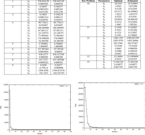
The optimal and estimated parameters of the NRMs ob-tained by the Jaya algorithm are displayed in Table III. These parameters correspond to the best RSS results. These results clearly show that the estimated parameters obtained by the Jaya algorithm are very close to the optimal values of the parameters.
The performance results for each benchmark regression model through various approaches, including PSO and Jaya, and when using four performance metrics are listed in Table IV. In this table, the best results in terms of success rate, average number of iterations, average time and accuracy are shown in bold face. We should note that the PSO method was performed for the control parameters of inertia weight w and acceleration parameters c1 and c2 as 0.4, 2 and 2, respectively. Jaya clearly had a better success rate than PSO in most cases. As a summary, optimisation methods PSO and Jaya achieved success rates of 49.97% and 73.45%, respectively, for all the benchmark regression models. How-ever, these figures, do not consider the required number of iterations. From Table IV, we can observe that the Jaya optimisation method achieved a high success rate for test problems 2, 3, 5, 6, 7, 11 and 13 with fewer iterations than the conventional PSO. Although the Jaya algorithm required a greater number of iterations than PSO for test problems 1, 4 and 8, the success rate with Jaya was far better than that of PSO. However, the PSO method has a high success rate for test problems 9, 10 and 14 with fewer iterations
than Jaya. Table IV also reveals that Jaya had a better computational time in most cases except for test problems 10 and 11, in which there was a small difference between PSO and Jaya. This result was due to the simplicity of the Jaya algorithm. Finally, the Jaya algorithm also produced better computational accuracy in most cases. Although the Jaya and PSO algorithms had low success rates for test problem 12, the computational accuracy with Jaya was better than with PSO.
The advantage by using of the Jaya algorithm to estimation of nonlinear regression parameters is that it produces reliable and high quality results for the RSS values and parameter estimates of the regression models with less computational effort (or time) and high accuracy. Furthermore, the Jaya algorithm requires minimal effort for parameter tuning (such as for population size and several iterations) as compared to other algorithms such as PSO which requires extensive computational experiments to achieve a good performance. However, the major concern of the Jaya algorithm is its slow rate of convergence on some test problems (i.e. 1, 4, 8, 9, 10, 12 and 14) because a sufficient number of iterations were required to reach the optimal value.
It can also be interesting to examine the convergence behavior of two algorithms, PSO and Jaya, against the number of iterations. For this reason, we selected to test the ENSO nonlinear model as a representative case. Figure 1 and Figure 2 show the RSS values of the PSO and Jaya algorithms during the process of optimisation against the first 100 iterations, respectively. From these results show that both algorithms have a similar convergence behavior, i.e., they converge after at most 9-10 iterations to their minimum RSS value. Similar findings are valid for the most nonlinear models.
IV. CONCLUSIONS
In this study, we presented and implemented an application of the Jaya optimisation algorithm for estimating nonlinear regression parameters. We tested the algorithm experimen-tally on a set of NRMs using the RSS as an optimisation criterion. Furthermore, we compared the Jaya algorithm with
IAENG International Journal of Applied Mathematics, 48:4, IJAM_48_4_09
TABLE II
RESULTS OBTAINED BY THEJAYA ALGORITHM FOR14 NRMS
Test Problem Optimal Best Worst Mean Std. Dev.
1 0.124550 0.124551 0.124551 0.124551 0.000000
2 513.048000 513.048029 513.048029 513.048029 0.000000
3 2384.477100 2384.477139 2384.477139 2384.477139 0.000000 4 1315.822243 1315.822243 197566.709165 70262.718043 47959.503464
5 0.004317 0.004317 0.004317 0.004317 0.000000
6 0.075465 0.075465 0.075465 0.075465 0.000000
7 0.040967 0.040967 0.040967 0.040967 0.000000
8 0.056419 0.056419 0.056419 0.056419 0.000000
9 0.000495 0.000496 0.051525 0.011367 0.016920
10 788.539787 788.554655 1151.362195 877.937102 97.793790
11 0.000308 0.000308 0.000308 0.000308 0.000000
12 5642.708240 5644.81766 15040.582619 8462.562326 2825.174219 13 1168.008877 1168.008877 1168.008877 1168.008877 0.000000
14 8.056523 8.056523 1033.305133 383.980950 498.230860
TABLE III
ESTIMATED PARAMETERS OF14 NRMS OBTAINED BY THEJAYA ALGORITHM
Test Problem Parameters Optimal Estimated
1 b0 238.942129 238.942130
b1 0.0005501 0.000550
2 b0 0.16657 0.166577
b1 0.0051653 0.005165
b2 0.012150 0.012150
3 b0 0.19027 0.190278
b1 0.0061314 0.006131
b2 0.010530 0.010531
4 b0 98.778211 98.778211
b1 0.010497 0.010497
b2 100.489906 100.489907 b3 67.481111 67.481111 b4 23.129773 23.129773 b5 71.994503 71.994503 b6 178.998050 178.99805 b7 18.389389 18.389389
5 b0 0.768862 0.768862
b1 3.860405 3.860406
6 b0 337.997461 337.99746
b1 0.0003903 0.00039
7 b0 636.4273 636.427258
b1 0.000208 0.000208
8 b0 437.3737 437.369706
b1 0.0003022 0.000302
9 b0 0.2020 0.20477
b1 -6.195e-6 -0.000006 b2 1204.4556 1184.833335 b3 -181.3427 -182.547197
0 20000 40000 60000 80000 100000 120000
0 10 20 30 40 50 60 70 80 90 100
RSS
Iteration
ENSO
Fig. 1. The RSS behavior of the PSO algorithm for ENSO model
TABLE III
ESTIMATED PARAMETERS OF14 NRMS OBTAINED BY THEJAYA ALGORITHM(CONTINUED)
Test Problem Parameters Optimal Estimated
10 b0 10.5107 10.510004
b1 3.0762 3.073296
b2 0.5328 0.533395
b3 44.3111 44.299963
b4 -1.6231 -1.633337
b5 0.5255 0.51916
b6 26.8876 26.896185
b7 0.2123 0.222564
b8 1.4967 1.502261
11 b0 0.1928 0.192807
b1 0.1913 0.191282
b2 0.1231 0.123057
b3 0.1361 0.136062
12 b0 1288.1397 1288.092709
b1 1491.0793 1492.26984 b2 583.2384 583.97267
b3 75.4166 75.55428
b4 0.9663 0.966956
b5 0.3980 0.398355
b6 0.0497 0.050114
13 b0 213.8094 213.809409
b1 0.5472 0.547237
14 b0 72.462238 72.462238
b1 2.618077 2.618077 b2 0.067359 0.067359
0 50000 100000 150000 200000 250000 300000 350000 400000
0 10 20 30 40 50 60 70 80 90 100
RSS
Iteration
[image:4.595.48.546.295.756.2]ENSO
Fig. 2. The RSS behavior of the Jaya algorithm for ENSO model
IAENG International Journal of Applied Mathematics, 48:4, IJAM_48_4_09
TABLE IV
RESULTS OFPSOANDJAYA ALGORITHMS FOR14 NRMS
Success rate (%) Average number of iterations Average time (in secs) Accuracy
Test Problem PSO Jaya PSO Jaya PSO Jaya PSO Jaya
1 98.33 100 845 1097 0.7070 0.6295 0.000001 0.000001
2 100.00 100.00 928 551 2.8255 1.9471 0.000029 0.000029
3 3.33 100.00 1469 602 10.8258 10.1816 0.510953 0.000039
4 0.00 33.33 380 1294 62.3886 44.8105 98668.688468 0.000000
5 100.00 100.00 697 303 0.3847 0.3763 0.000000 0.000000
6 1.66 100.00 1872 989 0.1480 0.1158 0.000234 0.000000
7 3.33 100.00 1469 959 0.2331 0.1799 0.000000 0.000000
8 20.00 100.00 243 930 0.1314 0.1233 0.000000 0.000000
9 100.00 1.66 975 1718 1.9938 1.1489 0.000000 0.000001
10 66.33 26.67 1520 1601 41.6046 42.9278 0.000013 0.015917 11 100.00 100.00 1183 501 0.1151 0.1152 0.000000 0.000000
12 0.00 0.00 152 1162 3.96 3.8811 318.825760 2.109424
13 6.66 100.00 430 221 0.2318 0.2143 0.006043 0.000000
14 100.00 66.67 1038 1340 0.3586 0.3219 0.000000 0.000000
Average 49.97 73.45
the PSO using several performance measures. We concluded that the Jaya algorithm represents a good candidate algo-rithm for effective parameter estimation with most NRMs because it provides stable and reliable results within less computational time. Furthermore, this proposed method can be applied to regression models that manage big data. Finally, this algorithm could be used to solve complex problems such as time-series analysis, social network analysis, and shape optimisation [14].
ACKNOWLEDGMENT
The author would like to thank the editor and the reviewers for their helpful comments and suggestions, which have improved the presentation of this paper. The computational experiments reported in this paper were performed at the Parallel and Distributed Processing Laboratory (PDP Lab) of the Department of Applied Informatics, University of Macedonia. The author would also like to thank the personnel of the PDP Lab.
REFERENCES
[1] M. Kapanoglu, I. O. Koc, and S. Erdogmus, “Genetic algorithms in parameter estimation for nonlinear regression models: an experimental approach,” Journal of Statistical Computation and Simulation, vol. 77, no. 10, pp. 851–867, 2007. [Online]. Available: https://doi.org/10.1080/10629360600688244
[2] V. S. Ozsoy and H. Orkcu, “Estimating the parameters of nonlinear regression models through particle swarm optimization,”
Gazi University Journal of Science, vol. 29, no. 1, pp. 187–199, 2016. [Online]. Available: http://dergipark.gov.tr/download/article-file/230923
[3] G. C. V. Ramadas and E. M. G. P. Fernandes, “Solving systems of nonlinear equations by Harmony Search,” in Proceedings of the 13th International Conference on Computational and Mathematical Methods in Science and Engineering, CMMSE 2013, 2013. [Online]. Available: https://core.ac.uk/download/pdf/55627383.pdf
[4] A. Minot, Y. M. Lu, and N. Li, “A distributed Gauss-Newton method for power system state estimation,” IEEE Transactions on Power Systems, vol. 31, no. 5, pp. 3804–3815, Sept 2016. [Online]. Available: https://ieeexplore.ieee.org/document/7337467/
[5] S. Liu, A. Bustin, D. Burshka, A. Menini, and F. Odille, “GPU implementation of Levenberg-Marquardt optimization for Ti mapping,” in2017 Computing in Cardiology (CinC), Sept 2017, pp. 1– 4. [Online]. Available: https://ieeexplore.ieee.org/document/8331434/ [6] R. V. Rao, “Jaya: A simple and new optimization algorithm
for solving constrained and unconstrained optimization problems,”
International Journal of Industrial Engineering Computations, vol. 7, no. 1, pp. 19–34, 2016. [Online]. Available: http://www.growingscience.com/ijiec/Vol7/IJIEC 2015 32.pdf
[7] R. V. Rao, D. P. Rai, and J. Balic, “A new optimization algorithm for parameter optimization of nano-finishing processes,” Scientia Iranica, 2016. [Online]. Available: http://scientiairanica.sharif.edu/article 4068.html
[8] W. Warid, H. Hizam, N. Mariun, and N. I. Abdul-Wahab, “Optimal power flow using the Jaya algorithm,”Energies, vol. 9, no. 9, p. 678, 2016. [Online]. Available: http://www.mdpi.com/1996-1073/9/9/678 [9] I. Kiv, J. Tvrdk, and R. Krpec, “Stochastic algorithms in
nonlinear regression,” Computational Statistics and Data Analysis, vol. 33, no. 3, pp. 277 – 290, 2000. [Online]. Available: http://www.sciencedirect.com/science/article/pii/S0167947399000596 [10] L. lai Li, L. Wang, and L. heng Liu, “An effective
hybrid PSOSA strategy for optimization and its application to parameter estimation,” Applied Mathematics and Computation, vol. 179, no. 1, pp. 135 – 146, 2006. [Online]. Available: http://www.sciencedirect.com/science/article/pii/S0096300305010155 [11] R. V. Rao and G. Waghmare, “A new optimization algorithm
for solving complex constrained design optimization problems,”
Engineering Optimization, vol. 49, no. 1, pp. 60–83, 2017. [Online]. Available: https://doi.org/10.1080/0305215X.2016.1164855
[12] NIST, nonlinear regression. [Online]. Available: https://www.itl.nist.gov/div898/strd/nls/nls main.shtml
[13] S. kai S. Fan, Y. chia Liang, and E. Zahara, “Hybrid simplex search and particle swarm optimization for the global optimization of multimodal functions,” Engineering Optimization, vol. 36, no. 4, pp. 401–418, 2004. [Online]. Available: https://doi.org/10.1080/0305215041000168521
[14] S. Skinner and H. Zare-Behtash, “State-of-the-art in aerody-namic shape optimisation methods,” Applied Soft Computing, vol. 62, pp. 933 – 962, 2018. [Online]. Available: http://www.sciencedirect.com/science/article/pii/S1568494617305690