High Fidelity Probe and Mitigation of Mirror Thermal
Fluctuations
Thesis by
Tara Chalermsongsak
In Partial Fulfillment of the Requirements for the Degree of
Doctor of Philosophy
California Institute of Technology Pasadena, California
2014
c 2014
Acknowledgments
Each day, after spending strenuous hours of lab work and about to call it a night, I liked to look around the setup of the work. Not only did I think about what could be improved or what to be fixed, but I also reminded myself about how far I had accomplished with a lot of help from several people who taught me all about the optic mounts on the table, electronic equipments, or even softwares for controlling the setup. I consider myself very fortunate to learn from many of the smartest people I have ever known over the years.
First, I have to thank Rana Adhikari for taking me under his wing and entrusting me to this exciting experiment, and for his patient for teaching someone who’s not the fastest learner like me. I’m also grateful for Eric Gustafson, another boss who always has indispensable advice on my work. I also thank Yanbei Chen, Kenneth Libbrecht, and Alan Weinstein for serving on my committee.
I learned many crucial lab skills from Frank Seifert whose help contributes significantly to my work. Also, I am grateful to Koji Arai, Peter King, Vladimir Degarchev, Matt Abernathy, Nicolas Smith, Steve Vass, Jamie Rollins, Jan Harms, Aidan Brooks, Alastair Heptonstall, Manasa Thirug-nanasambandamand, and Larry Price. They were always ready to answer any questions I had. Without them, I would be like a blind man roaming in a minefield.
The work would not be made possible without all the electronic supports from LIGO engineers, especially, Daniel Sigg, Rich Abbott, and Charles Osthelder. They have been very kind to help me through these years.
Also, I like to thank all the TNI members, Riccardo DeSalvo, Eric Black, Akira Villar, and Greg Ogin from their guidance during my first few years at Caltech. Their researches motivated my study in the following years.
I appreciate all the help from my grad student fellows, David Yeaton–Massey, Jenne Driggers, Kiwamu Izumi, Zach Korth, Eric Quintero, Denis Martynov, and Evan Hall. I used to struggle with problems alone, and it was devastating. They taught me how to help and learn from each others and the value of teamwork.
I’m also indebted to all Physics and LIGO members, especially Donna Driscoll, Julie Hiroto, and Gina Salone for their help and support on various works.
I also have to thank Laura F. Kim, Daniel Yolder and Caltech ISP team who have helped me with all the issues for an international student like me.
I am lucky to know some Caltech Thai students who always share laugh and cry with me. Special thanks to Tichakorn Wongpiromsarn and Piti Ongmongkolkul for several useful helps and discussions in maths and physics.
Abstract
Thermal noise arising from mechanical loss in high reflective dielectric coatings is a significant source of noise in precision optical measurements. In particular, Advanced LIGO, a large scale interferometer aiming to observed gravitational wave, is expected to be limited by coating thermal noise in the most sensitive region around 30–300 Hz. Various theoretical calculations for predicting coating Brownian noise have been proposed. However, due to the relatively limited knowledge of the coating material properties, an accurate approximation of the noise cannot be achieved. A testbed that can directly observed coating thermal noise close to Advanced LIGO band will serve as an indispensable tool to verify the calculations, study material properties of the coating, and estimate the detector’s performance.
This dissertation reports a setup that has sensitivity to observe wide band (10 Hz to 1 kHz) thermal noise from fused silica/tantala coating at room temperature from fixed-spacer Fabry–Perot cavities. Important fundamental noises and technical noises associated with the setup are discussed. The coating loss obtained from the measurement agrees with results reported in the literature.
The setup serves as a testbed to study thermal noise in high reflective mirrors from different materials. One example is a heterostructure of AlxGa1−xAs (AlGaAs). An optimized design to
Contents
Acknowledgments iii
Abstract v
1 Introduction to Thermal Noise 1
1.1 Thermal Noise in Various Measurements . . . 1
1.1.1 The Brownian Movement . . . 1
1.1.2 Johnson-Nyquist Noise. . . 2
1.1.3 Micro Electromechanical Systems: MEMS . . . 3
1.1.4 Torsion Pendulum . . . 3
1.1.5 Optical Clock . . . 4
1.1.6 Laser Interferometer Gravitational Wave Observatory . . . 4
1.1.6.1 A Short Review on Gravitational Wave . . . 5
1.1.6.2 LIGO Setup . . . 6
1.1.6.3 Thermal Noise in LIGO . . . 6
1.2 Direct Observations of Thermal Noise in High Reflective Mirrors . . . 8
1.2.1 Previous Coating Thermal Noise Measurements. . . 8
1.2.2 Coating Brownian Noise from Fixed Spacer Fabry–Perot Cavity . . . 9
2 Thermal Noise in Fixed–Spacer Fabry–Perot Cavity 11 2.1 Fluctuation-Dissipation Theorem . . . 13
2.2 Direct Approach . . . 14
2.3 Two Kinds of Thermal Noise . . . 14
2.3.1 Brownian Thermal Noise . . . 15
2.3.2 Thermodynamic Noise . . . 15
2.4 Thermal Noise in Substrate . . . 16
2.4.1 Brownian Noise in Substrate . . . 17
2.4.2 Thermoelastic Noise in Substrate . . . 17
2.5 Thermal Noise in Coatings . . . 19
2.5.1 Brownian Noise in Coatings . . . 19
2.5.2 Thermo–Optic Noise in Coatings . . . 21
2.6 Thermal Noise in Spacer . . . 23
2.6.1 Brownian Noise in Spacer . . . 23
2.6.2 Thermoelastic Noise in Spacer . . . 24
2.7 Photothermal Noise: Absorption from Shot Noise and Intensity Noise . . . 25
2.8 Noise in the Bonding between a Mirror and a Spacer . . . 26
2.8.1 Optical Contact . . . 27
2.8.2 How to Measure Mechanical Loss in Optical Contact . . . 27
2.9 How to Reduce Thermal Noise . . . 28
2.9.1 Lower Temperature . . . 28
2.9.2 Lower Loss . . . 29
2.9.3 Different Beam Shape . . . 30
2.9.4 No Coating Cavity . . . 30
3 Experimental Setup 32 3.1 Optical Cavity as a Frequency Reference . . . 33
3.2 Prototype Setup . . . 35
3.2.1 8–inch Reference Cavities . . . 35
3.2.2 Setup Layout . . . 37
3.2.3 Result from the Prototype Setup . . . 40
3.3 Two Laser Setup with 1.45 Inch Cavities. . . 42
3.3.1 1.45 Inch Reference Cavities. . . 42
3.3.2 Overall Explanation of The Two–Laser Setup . . . 43
3.3.3 Result from 1.45 Inch Cavities . . . 46
3.4 Discussion . . . 46
4 Technical Noise in the Setups 49 4.1 Seismic Noise . . . 49
4.1.1 Coupling from Seismic to Displacement Noise . . . 49
4.1.2 Scattered Light and Seismic Isolation in the Setup . . . 51
4.2 Mechanical Peaks from Opto–Mechanical Components . . . 51
4.3 PDH Lock: Shot Noise . . . 53
4.4 PDH Lock: Electronic Noise. . . 55
4.5 PDH Lock: Residual Amplitude Modulation. . . 56
4.7 Photothermal Noise . . . 61
4.8 Noise from Ambient Temperature. . . 62
5 AlGaAs Crystalline Coatings 63 5.1 History of AlGaAs Usage . . . 63
5.2 Thermo–Optic Noise and Coatings Optimization . . . 64
5.2.1 Thermal Noise in AlGaAs Coatings. . . 65
5.2.2 Optimization Consideration . . . 66
5.2.3 Uncertainties in Material Parameters. . . 69
5.2.4 Errors Due to Manufacturing Process . . . 70
5.2.5 Optimization Method . . . 71
5.2.6 Cavity Parameters . . . 78
5.3 Implications for Advanced LIGO . . . 78
6 Future Upgrade and Application 83 6.1 Future Upgrade. . . 83
6.1.1 Improvement in Sensitivity at Low Frequency . . . 83
6.1.2 Improvement in Sensitivity at High Frequency . . . 85
6.2 Application: Frequency Stabilized Light Source . . . 87
6.2.1 Laser Gyroscope . . . 87
6.2.2 Crackle . . . 88
6.2.3 External Cavity Diode Laser . . . 89
A Comparison with Other Experiments 91 B Frequency Stabilization Servo 95 C Material parameters for SiO2/Ta2O5 and AlGaAs 99 C.1 Table of Parameters . . . 99
C.2 Uncertainties in Parameters . . . 99
C.3 Note for AlGaAs . . . 100
D High Reflective Coating Structure and its Average Properties 101 D.1 Why Half Wave Cap? . . . 101
D.2 Averaged Material Parameters for Coatings . . . 102
E 1.45 Inch Reference Cavity: Design and Assembly 104 E.1 Choosing Cavity Length . . . 104
E.3 Eigenmode study . . . 110
E.4 Searching for Optimum Support Point with COMSOL . . . 111
E.5 Mount Design and Assembly . . . 111
F Pre-Mode Cleaner Cavity 117 F.1 Eigenmode Study . . . 117
G Mathematical Note 119 G.1 Note About Fabry–Perot Cavity . . . 119
G.2 Temperature Fluctuations for TO Calculation . . . 120
G.3 Error Analysis of the Measurement . . . 122
G.4 Bayesian Analysis. . . 123
Chapter 1
Introduction to Thermal Noise
For a system in thermal equilibrium at temperature T, the Equipartition Theorem tells us that the average kinetic from each degree of freedom will be equal to 12kBT. For example, a 1-D mass-spring
system with only one degree of freedom, will oscillate with an average energy of 12kBT. At first,
it seems that the only movement will be x(t) =x0sin (2πf t), a perfect sinusoidal motion with its
frequencyf determined solely by the massmand the spring constantk. However, if the spring has a mechanical loss which can be written as an imaginary part of the spring constantk=k0(1 +iφ),
whereφ1, this loss will cause an off-resonant motion that creates noise in other frequencies. In the next chapter, we will discuss more about Fluctuation-Dissipation theorem, which explains how loss and fluctuation in a system are related (for this chapter, we can just remember that a system that can dissipate the input energy, can exhibit fluctuations as in the mass-spring system).
This minute motion manifests itself in a larger scale and has been observed in various experiments, and becomes one of the fundamental limiting sensitivity for sensitive measurements. This chapter will give some examples of thermal noise in measurements.
1.1
Thermal Noise in Various Measurements
1.1.1
The Brownian Movement
When small particles (e.g., pollen grains) are suspended in still water with no influence from the sur-rounding, the particles will move randomly. This motion was observed in 1827 by Robert Brown [1] and it was named as Brownian motion. The particle’s movement originates from continuous random collisions from the surrounding water molecules that move due to their thermal energykBT. It had
1.1.2
Johnson-Nyquist Noise
Voltage noise in resistors relating to the temperature had been observed by Johnson in 1928 [5] (Fig. 1.1), and explained by Nyquist in the same year [6]. The cause is electrons’ movement inside a resistor due to thermal agitation. Nyquist proved it using an argument that certain wave pattens can be formed in a system of two resistors joined by two transmission lines together with the Equipartition Theorem stating that each degree of freedom has an energy equal tokBT. In general,
the power spectral density of the voltage noise is
V2(f) = 4hf∆f
exp[khf
BT]−1
(1.1)
Usually, in most cases when hf kBT ( For example, T = 300K, f can be up to 100GHz),
Eq.1.1is reduced to a more familiar form,
[image:11.612.188.464.325.543.2]V2(f) = 4RkBT∆f. (1.2)
Figure 1.1: Apparent power[V2/R] vs. temperature, for Advance wire resistances [5]
1.1.3
Micro Electromechanical Systems: MEMS
Developments in micro-machining process make small tools at micron scale possible. Typically, they consist of simple mechanical devices (e.g., a mass-spring system, a cantilever blade) with sizes of around 100 to 1000 microns, (see Fig.1.2). These devices are suitable for space-limited applications because they are small and light. Similar to any mechanical systems, they are also subject to thermal noise due to intrinsic mechanical losses in the material [13]. Although the devices are usually limited by the related electrical noise and systematic errors, mechanical thermal noise sets the fundamental limit of the devices and it is important to characterize them for the improvement of the higher accuracy devices. Some examples of MEMS devices and their thermal noise considerations can be found in Ref. [14] for a frequency selective device using the mechanical resonance of a small cantilever blade, Ref [15] for a gyroscope, and Ref. [16] for a Fabry–Perot tunable etalon.
Figure 1.2: Left, a schematic diagram of a capacitive MEMS accelerometer. Right, a micrograph of the ADXL50 MEMS accelerometer’s structure. Credit: www.sensorsmag.com
1.1.4
Torsion Pendulum
Torsion pendula can be used to study the influence of solar eclipses on some mechanical processes on earth [22, 23], although, in this case, they are not used for determining any small forces. The oscillation period of the torsion pendulum increases during the solar eclipse. This phenomenon has not been properly explained.
Similar to other sensitive measurements, a torsion pendulum is subject to thermal noise due to loss in the torsion spring. A direct measurement to observe thermal noise in a torsion pendulum was done with a polyamide Nylon wire, and the result was in good agreement with the Fluctuation-Dissipation theorem [24].
1.1.5
Optical Clock
The optical clock [25] has been quickly developed as another frequency standard, which is important in various fields (e.g., primary standards, time distributions services, global navigation satellite sys-tems (GPS)). Three main components of an optical clock are (1) a highly stable reference frequency (a narrow optical absorption line in an atom or ion)1, (2) a laser (local oscillator), which is locked
to that reference frequency, and (3) a femtosecond comb for measuring the frequency of the laser. The laser has two important tasks; it must probe the reference transition (the atomic system) while introducing minimal noise, and it must act temporarily as stable frequency reference to maintain the short to medium term stability of the frequency reference [27]. To do this, the laser is also frequency locked to a reference cavity. Thermal noise in that reference cavity, which will be studied in details in this dissertation, becomes one of the main limiting noise source of the laser’s performance.
1.1.6
Laser Interferometer Gravitational Wave Observatory
The existence of gravitational waves was predicted as a consequence of the theory of general relativ-ity [28,29,30]. As a gravitational wave propagates through space, it contracts and expands the space periodically. Although observations on the displacement due the warped space has never been made because of their extremely weak signals, there is strong evidence suggesting their existence. In 1974, a piece of evidence of gravitational waves was observed from the shrinking orbit of a binary system of two neutron stars, PSR1913+16 (one of which is also a pulsar) due to energy loss in the form of gravitational waves [31,32]. The prediction of general relativity agrees with the measurement to accuracy of about 0.1 percent, after 30 years of data [33].
Another example is recent news at the time of writing this dissertation, researchers from the BICEP2 collaboration [34] have announced they found evidence of cosmic inflation and reported the image of gravitational waves from the Big Bang by observing the B-modes polarization of the cosmic 1For optical lattice clock [26] the atoms are kept into an optical lattice instead of trapped by laser cooling. The
microwave background (CMB) [35]. This new finding is currently under peer review for scientific confirmation. Nevertheless, gravitational wave is real.
In 1990s, scientists proposed a large scale interferometer to measure gravitational wave (LIGO2[36]).
The configuration based on a Michelson interferometer with 4–km arms. Later, a network of ground based observatories (VIRGO3 [37], GEO4 [38], KAGRA5 [39])have been built around the world to
increase the confidence and to pinpoint a location of an event. Some possible GW sources that will be detectable by the observatories are: signals from binaries, coalescing binaries, supernovae, or stochastic signals.
1.1.6.1 A Short Review on Gravitational Wave
In General Relativity, space-time is described by the mass-energy following the Einstein’s field equation:
Rµν−
1
2Rgµν = 8πG
c4 Tµν. (1.3)
Rµν is the Ricci curvature tensor, R is the scalar curvature,gµν is the metric tensor, which explains
the structure of the space-time. The stress-energy tensor Tµν describes the density and flux of
energy, mass, and momentum in space-time. See Ref. [40] for more details. In a place far away from the presence of mass or energy, the space time metricgµν can be approximated as
gµν =ηµν+hµν with|hµν| 1, (1.4)
where ηµν is the flat space-time (Minkowski) metric and hµν is a small perturbation due to the
gravitational wave. In free space (Tµν = 0), substituting this space time metric to Einstein’s field
equations and using an appropriate gauge choice (transverse traceless gauge), the Einstein’s field equation reduces to a wave equation forh:
∇2h
µν =
∂2h
µν
∂t2 (1.5)
Due to the constraints of the choice of gauge and the field equation, hµν can be decomposed into
two linearly independent modes, which areh+ and h×. Conventionally, h+ squeezes and stretches
along the ˆxand ˆy directions while h× will stretch and squeeze along ˆx+ ˆy and ˆx−yˆ directions. If a gravitational wave with h+ polarization propagates along the z-axis, an object with length L
oriented alongxory axes will have the maximum displacement due to the strain equal to
∆L=Lh+. (1.6)
2http://www.ligo.org
3
http://www.ego-gw.it/virgodescription/pag_4.html
4http://www.geo600.org
For a binary system with its orbital plane being parallel to x-y plane, the strainhis [41]:
h(z, t) = −4G
2M 1M2
c4rz cos(2πf(z−ct)/c), (1.7)
M1,M2are the masses of the two bodies separated by distancer. For the binary system PSR1913+16,
M1 = 1.44M, M2 = 1.39M, and M is the solar mass,r = 2.3 light seconds, z = 20,000 light years. Substituting these numbers in Eq.1.7, we get the strain around 1.3×10⁻²². However, the wave frequency is around 0.1 mHz, making it undetectable for the current sensitivity of the ground based observatory, see Fig.1.4.
1.1.6.2 LIGO Setup
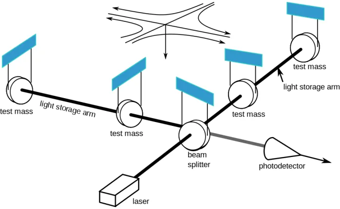
[image:15.612.149.498.381.596.2]Due to the nature of a gravitational wave that warps space-time as it propagates, a Michelson interferometer can be a suitable tool for detecting the wave. A schematic diagram of LIGO is shown in Fig.1.3. The input laser is separated into two directions orthogonal to each other. They bounce off of the high reflective mirrors at the end of each arm and recombine at the output. The differential length between the two arms, induced by the passing wave, results in the varying power of the output monitored by a photodiode.
Figure 1.3: A simplified schematic diagram of LIGO. It is a Michelson interferometer with a Fabry–Perot cavity in each arm. The test masses are suspended for seismic isolations.
1.1.6.3 Thermal Noise in LIGO
motion on the ground that shakes the test masses’ positions will prevent LIGO from detecting gravitational waves at frequencies below 10 Hz. The estimated noise budget of Advanced LIGO is shown in Fig.1.46.
101 102 103
10−24
10−23
10−22
10−21
Frequency [Hz]
Strain [1/
√
Hz]
Quantum noise Seismic noise Gravity Gradients
Suspension thermal noise Coating Brownian noise Coating Thermo−optic noise Substrate Brownian noise Excess Gas
[image:16.612.148.497.136.354.2]Total noise
Figure 1.4: Baseline Advanced LIGO’s noise budget (GWINC v2.0). 125 W input power [43]. Coating Brownian noise is plotted in confidence interval where uncertainties of coatings’ mechanical loss angles and Young’s moduli are taken into consideration.
Thermal noise comes into LIGO sensitivity in two places, the suspensions and the test masses.
• Thermal noise in suspension
To reduce seismic noise due to the ground’s motion, LIGO test masses are suspended with multiple stages for seismic isolations [44]. Similar to thermal noise in a torsion pendulum, the suspension wires joining each stage also come with thermal noise because of the loss in the wires [45]. Another example of thermal noise measurement in a mechanical flexure suspension can be found in Ref. [46]. Not only the losses in the suspension wires that contribute to the displacement noise, but also the dissipation associated with the whole suspension system, e.g., the magnet-coil actuators, joints between a suspension wire and the test mass, maraging blade springs, gas damping due to residual gas molecules, or electrostatic damping due to currents induced in structures and charges. These noise sources must be minimized to achieve the target sensitivity.
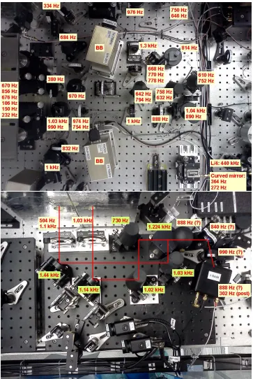
crumbling paper. An experiment to test this phenomenon in maraging steel blades is on going at Caltech [47]. The device under test will be driven at sub hertz frequency in order to observe the noise in audio band interferometrically.
• Thermal Noise in Test Masses
As the output from the asymmetric port of the beam splitter is directly related to the differen-tial arm lengths, thermal noise in the test masses changes the test mass surfaces’ positions and directly couples to the output signal. It is estimated that the sensitivity of Advanced LIGO in the most sensitive band (30 Hz to 300 Hz) will be limited by thermal noise in the high reflective coatings, see Fig. 1.4. Although quantum noise is another dominating noise source that covers the whole measurement bandwidth, it can be reduced below coating thermal noise by frequency dependent squeezed light [48,49]. The radiation pressure noise at low frequencies can be reduced by amplitude squeezing, while the shot noise limit at high frequencies can be reduced by phase squeezing.
Since coating thermal noise has been identified as an important limiting noise source, research on coatings has rapidly grown. Many groups have developed mathematical models to calculate coating thermal noise [50,51,52, 53]. However, due to the coating’s multilayer structure and uncertainties in the thin film material parameters (e.g., Young’s moduli, Poisson ratios, and loss angles), thermal noise in coatings is not thoroughly understood. For this reason, a test facility, which can measure coating thermal noise with high signal-to-noise ratio across a wide frequency band relevant to Advanced LIGO, is necessary for a comprehensive verification. The setup for this coating thermal noise measurement will be the one of the main topics in this dissertation.
1.2
Direct Observations of Thermal Noise in High Reflective
Mirrors
1.2.1
Previous Coating Thermal Noise Measurements
Advanced LIGO performance since it is predicted to be limited by coating thermal noise in this bandwidth. Additionally, the setup similar to that of TNI requires larger, heavier substrates to overcome seismic noise for measurements at lower frequencies. Big custom made substrates are expensive for testing several samples. A setup that uses smaller commercially available substrates is preferred. An alternative setup is needed to overcome such issues.
Figure 1.5: Inside of TNI’s main vacuum chamber, ca. 2007. The suspended test masses are on the left, the triangular Mode Cleaner cavity is on the right. Picture credit: Akira Villar
1.2.2
Coating Brownian Noise from Fixed Spacer Fabry–Perot Cavity
In the field of optical frequency metrology, a fixed–spacer Fabry–Perot cavity (see Fig.1.6) is typically used as a stable reference for locking laser frequency. By designing the shape of the spacer, and searching for vibration insensitive support points, several groups have demonstrated that the total displacement noise of a rigid cavity can be very close to the thermal noise limit from the high mirror coating at frequencies around 0.01 - 1 Hz [56,57,58]. However, none have reported Brownian thermal noise in the frequency band relevant to ground based GW detectors.7
This motivates us to develop a testbed that can directly observe coating thermal noise in the 10 Hz to 1 kHz bandwidth using fixed spacer Fabry–Perot cavities and standard 1 inch diameter substrates. Fortunately, the spacer does not introduce a lot of excess displacement noise. Thermal noise associated with a spacer made from fused silica is predicted to be much smaller than that in dielectric coatings [59,60]. More details are discussed in chapter2.
Another advantage of the fixed spacer setup, besides the lower cost for the samples, is the shorter turnaround time because of commercially available substrates and the less complicated suspension
system. It takes approximately a month for each set of samples to be installed and measured. In addition, as the measurement can be done optically from the transmitted beams, the calibration is relatively simple (cf. section4.6) compared to the readout technique used in TNI measurement [55]. Furthermore, an error related to spot size and cavity’s length in a fixed–spacer cavity will be less than that of a suspended cavity. Better knowledge on the spot size leads to more accurate coating thermal noise calculation. In the next chapter, thermal noise in all parts of a fixed-spacer Fabry–Perot cavity will be discussed in detail.
Chapter 2
Thermal Noise in Fixed–Spacer
Fabry–Perot Cavity
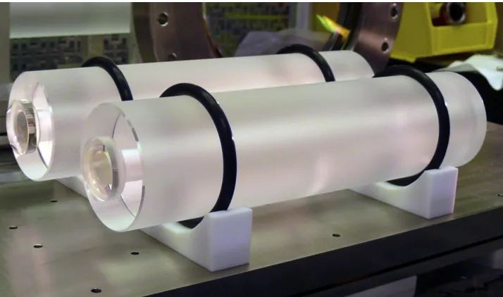
Typically, a Fabry–Perot cavity consists of three parts: two mirror substrates, high reflective coatings deposited on the substrates, and a spacer with a bore hole along the beam line axis for the beam to propagate in vacuum. The substrates are usually optically bonded to the spacer on both ends, as shown in Fig.2.1. To use a fixed-spacer Fabry–Perot cavity in a coating thermal noise measurement, all fundamental noises related to the cavity have to be considered.
Figure 2.1: Assembly of a 1.45-in spacer used in this dissertation. The substrates are optically contacted on both ends of the spacer. The vent hole for using the cavity in a vacuum system can be seen.
Symbol Name unit
f temporal frequency Hz
c light speed in vacuum m/s
Sx(f) single-sided power spectral density m2/Hz
kB Boltzmann constant J/K
T Mean temperature K
C Heat capacity per volume J/Km3
κ Thermal conductivity W/mK
Y Young’s modulus N/m2
σ Poisson’s ratio
α Thermal expansion coefficient 1/K β Thermorefractive coefficient,∂n/∂T 1/K
n Refractive index
λ Beam wavelength m
ν carrier frequency Hz
ω0 Beam radius (1/e2power) m
d Coating thickness m
φ Mechanical loss angle
L cavity length m
2.1
Fluctuation-Dissipation Theorem
Let’s look back to Brownian motion of a particle in water. When the particle is left alone, water molecules randomly and continuously collide with it and move the particle around. On the other hand, if the particle is dragged through the water, these random collisions from the water will act as a frictional force trying to dissipate the particle’s kinetic energy. From these two situations, we see that the fluctuation of the particle’s position (or velocity) and the dissipation of the particle’s energy under the influence of an external force are both caused by the same phenomenon: the collisions with the surrounding water molecules. This implies that the fluctuation and the dissipation are related, as they share the same origin. The coupling between them given by the Fluctuation-Dissipation Theorem (FDT) [61] is1
Sx(f) =
kBT
π2f2Re[Y(f)], (2.1)
wheref is Fourier temporal frequency,Y(f) is the mechanical admittance associated withx(t). The admittance can be computed by looking at a generalized forceF(t) that drives the system in one of the generalized coordinates,x(t). The admittance is the Fourier transform of the derivative ofx(t) divided by the applied force which is
Y(f) = x˙(f)
F(f) =
2πif x(f)
F(f) . (2.2)
Let’s see an example in a mass-spring system. A mass m is attached to a spring with spring constantk(1 +iφ). The equation of motion can be written as
F =k(1 +iφ)x+mx.¨ (2.3)
The equation can be transformed to the frequency domain via a Laplace transformation. Rearrange the equation to get,
Y = x˙
F =
iω
k−ω2m+ikφ (2.4a)
=(iω)(k−ω
2m−ikφ)
(k−ω2m)2+k2φ2 , and (2.4b)
Re[Y] = kφω
(k−ω2m)2+k2φ2, (2.4c)
whereω= 2πf. Substituting this back into Eq. 2.1, in the limit of 2πf qk
m we get
1A comprehensives review about the Fluctuation–Dissipation can be found in Ref. [62], and an introduction to a
Sx(f) =
2kBT
πf φ
k. (2.5)
This equation captures all significant characteristics of thermal Brownian noise. It is directly pro-portional to the temperature and the loss of the system. It is inversely propro-portional to the frequency and the stiffness of the material (spring constant). In general,φcan be frequency and temperature dependent.
2.2
Direct Approach
Thermal noise in a beam-optic system is not as simple as the mass-spring example. Previous calculations to determine thermal noise were done by a modal expansion, for example, in a suspension system [64], or in a mirror of a laser interferometer gravitational-wave detector [65]. This method calculates the admittance and sums up contributions from all vibration modes contributing to the strain of the system. However, it is computationally expensive, complicated, and the result is not guaranteed to converge [66]. Additionally, this method cannot handle non-uniform loss in the substrate. The dielectric coatings turn out to be more lossy than the mirror substrate. As the coating is closer to the beam than the substrate, its effect contributes to the surface fluctuation even more. Instead of using modal expansion, one can use the so-called “direct approach” to compute Re[Y(f)]. This was introduced by Gonz´alez and Saulson [67] for computing thermal noise in suspensions, and was later applied to a laser mirror by Levin [66]. In this approach, one calculates the thermal noise by applying a cyclic force which causes power dissipation in a lossy system. With the FDT, the dissipated powerWdiss and the PSDSxare related by
Sx(f) =
2kBT
π2f2
Wdiss
F2
0
, (2.6)
where F0 is the magnitude of the applied force to calculate the dissipated power. In the case of
mirror whose position is interrogated by a laser beam, the cyclic “force” applied is a pressure with the same profile as the intensity of the beam.
2.3
Two Kinds of Thermal Noise
which create temperature fluctuations in a system.
2.3.1
Brownian Thermal Noise
Mechanical loss arises from the internal structure of a material, such as impurities or dislocations [69]. It is represented by introducing an imaginary part to the Young’s modulus of the material: E =
E0(1 +iφ). The quantity φis referred to as theloss angle, and may be temperature and frequency
dependent. When a sinusoidal force is applied to a system subject to mechanical loss, the dissipated power due to the applied force is given as [66]
Wdiss = 2πf U0φ, (2.7)
whereU0 is the maximum energy of elastic deformation. The loss angleφis equal to 1/Q, whereQ
is the quality factor. In general,Qcan be measured from a ring down measurement: an amplitude of an oscillation with resonant frequencyf0decays over time asA(t) =A(0)Exp[i2πf0t]Exp[−tπf0/Q].
If one is interested only in frequencies f below the first mechanical resonance frequency of the system (as is the case with our reference cavities), it is sufficient to compute the stored energyU0 in
the presence of a static force. The problem of evaluatingWdiss then reduces to a single elastostatic
computation, which can be carried out with finite element analysis (FEA) if necessary. Together with Eq.2.6, one can then calculate the Brownian contribution to the apparent position fluctuation of the mirror as sensed by a laser beam interrogating the mirror surface.
2.3.2
Thermodynamic Noise
In contrast to Brownian noise, thermo–optic noise is related to thermal, rather than mechanical, dissipation; it arises from fluctuations in the temperature field T(r, t) throughout the mirror [70]. In classical solid state thermodynamics, these fluctuations are not correlated with the volume fluc-tuations driven by Brownian noise. The two effects have to be summed incoherently.
In general, for a volume V, the total variance of temperature fluctuations can be described by [71]
< δT2>=kBT
2
CV . (2.8)
With non-zero thermal expansionα, and thermorefractiveβ, in coatings, a mirror and a spacer, the thermal fluctuation is converted into displacement noise or phase noise as the beam is reflected off of the mirror surface.
the mirror through the equation of static stress balance [75]
∇(∇ ·u) + (1−2σ)∇2u=−2α(1 +σ)∇δT, (2.9)
where u is the displacement vector of the mirror body due to the applied pressure. Then, the temperature perturbation evolves according to the thermal diffusion equation as [75]
∂(δT)
∂t −
κ
C∇
2(δT) = −αY T
C(1−2σ)
∂(∇ ·u)
∂t . (2.10)
Finally, the power dissipation due to the heat flow caused by the temperature gradient is given by the expression [75, Eq. 35.1]
Wdiss=
TdS
dt
=
Z
d3rκ
T(∇δT)
2
. (2.11)
Here T is the unperturbed temperature of the system andδT is the temperature perturbation due to the applied forceF0. The entropyS of the system changes due to the heat flux−κ∇(δT), and
the angle brackets denote an average over the period of oscillation of the force. By substituting Eq.2.11into Eq.2.6, we can obtain the temperature fluctuation on the mirror sensed by a Gaussian beam. This fluctuation couples into the electromagnetic response of the mirror viaαandβ.
In the literature, the term “thermoelastic noise” refers to physical displacement noise of the mirror’s surface position due to thermal expansion of the substate and the coating [76,72,77, 78]. In a beam-optic system, the change of the mirror position causes the phase shift of the reflected beam. On the other hand, “thermorefractive noise” refers to the phase fluctuation of the beam as it propagates through or reflects off the mirror (the path length of the beam changes even though the mirror surface position is fixed), and it is a combined effect of bothα and β. This is a slight misnomer, and it will be emphasized again.Since both thermoelastic and thermorefractive noises arise from a common origin, they are computed in a coherent fashion and the combined effect is called thermo–optic noise [74].
2.4
Thermal Noise in Substrate
2.4.1
Brownian Noise in Substrate
By using the direct approach, Brownian noise from a substrate as sensed by a Gaussian beam is given as [66],
Sx(f) =
2kBT
π3/2f
1−σ2s
w0Ys
φs. (2.12)
The result here is obtained from a half-infinite model, where the spot size is much smaller than the mirror size. Corrections for a finite size mirror are given in Ref. [72]. For our case, where spot sizes will be on the order of 200-300 µm, with 1 inch diameter and 0.25 inch thick substrates, the correction is negligible.
2.4.2
Thermoelastic Noise in Substrate
For Initial LIGO, the test masses were made of fused silica. In hopes of improving the sensitivity of the detector, scientists had proposed to switch test masses’ material from fused silica to sapphire due to its lower mechanical loss. However, Braginsky et al. [76] pointed out that thermoelastic noise had to be taken into consideration. As a result, a sapphire substrate was predicted to have higher total thermal noise than that of a fused silica substrate.
For the case of a half-infinite substrate in the adiabatic limitlthw0, wherelth= p
κs/(2πCsf)
is the thermal diffusion length at frequencyf, andκsandCsare, respectively, the thermal
conduc-tivity and the heat capacity per unit volume of the substrate, thermoelastic noise in substrate can be expressed as
SxT Esub(f) =
4kBT2αs2(1 +σs)2κs
√
π5C2
sw30f2
. (2.13)
Later, a non-adiabatic correction for low frequencies and small beam sizes was computed by Cerdonio et al. [77, Eq. 20], with some minor corrections as stated in Ref. [54,79] :
Sx(subTE)(f) = 4kBT
2
√
π
α2s 1 +σs
2
w0
κs
J f /fT
, (2.14)
wherefT=κs/πw2Cs, andJ(f /fT) is a non-elementary function whose asymptotes are 2/ 3 p
πf /fT
forf /fT1 and 1/ f /fT
2
forf /fT1; the full expression is
J(f /fT) =
2
π
1/2Z∞
0 du ∞ Z −∞ dv u
3e−u2/2
(u2+v2)
(u2+v2)2+ (f /f T)2
. (2.15)
At f fT, or in the adiabatic limit, Eq. 2.14 reduces to Eq. 2.13. The simplified equation
presents how thermoelastic noise level changes explicitly with the spot size and frequency.
tempera-ture [79], and found a good agreement with the theoretical calculation, showing that sapphire, even with lower mechanical loss than that of fused silica, has a higher total noise level due to thermoelastic noise.
2.4.3
Thermo–Optic Noise in Substrate
In a Fabry–Perot cavity topology, the beam passes through each substrate only once. Hence, thermo–optic noise in the substrate is usually much smaller than other thermal noise in the cavity. An analytical result for thermo–optic noise in a finite–sized cylindrical substrate sensed by a Gaus-sian beam is given in Ref. [80]. The frequency noise on the signal due to this effect is on the order of 10−7Hz/√Hzwhich will be negligible for our setup.
100 101 102 103 104 105 10−9
10−8 10−7
Frequency [Hz]
Frequency noise [Hz/rtHz]
TR noise in substrate, fused silica 300um beam size
Figure 2.2: Frequency noise of the beam passing through a quarter inch thick fused silica substrate. It is negligible compared to other noise source as shown in Fig.3.5and Fig.3.9.
Note that the “thermo–optic” noise calculation in Ref. [80] only takes the phase noise due toβ
(∂n/∂T) into account (it is also calledthermoref ractivenoise in the original paper). In reality, the
2.5
Thermal Noise in Coatings
One of the most important conclusions derived from the direct approach calculation is that the loss from the reflecting surface contributes to the noise significantly [66]. As a result, attention shifted to study more about the dielectric coatings. The coatings are usually more lossy than the bulk substrate, so they are expected to have higher thermal noise. Additionally, because of the multilayer structure and how light interacts within the coatings, thermal noise inside the coatings becomes more complicated, as we will see in this section.
2.5.1
Brownian Noise in Coatings
Brownian thermal noise in a thin film on a half-infinite substrate can be expressed as [50]
Sx(cBR)(f) =
4kBT
π2f
(1 +σs)(1−2σs)
Es
d
w2
0
φc, (2.16)
wheredis the total thickness of the coating, andφc is the coating’s loss angle.
This equation assumes that the elastic properties of substrate and the thin coating are the same, and that all the coating properties are isotropic. Due to the multilayer structure of the amorphous materials, the coating loss and elastic properties may be anisotropic. For this reason, authors such as Harry et al. [51] decompose coating loss and elastic deformation into parallel (k) and perpendicular (⊥) directions relative to the mirror normal. Then, in accordance with Eq. 2.7, the total dissipated energy can be written asWdiss= 2πf(U⊥φ⊥+Ukφk). The stored elastic energyU⊥ andUk can be calculated in the cylindrical coordinate. The spectral density is given as
Sxcoating(f) =2kBT
π2f
1−σ2
ω2
0Y
× d
Y Yc(1−2σc)(1−σ2)
×
Yc2(1 +σ)2(1−2σ)2φk
+Y Ycσc(1 +σ)(1 +σc)(1−2σ)(φk−φ⊥) +Y2(1 +σc)2(1−2σc)2φ⊥
.
(2.17)
This equation assumes that the coating’s Young’s modulus is isotropic: the modulus is the same in both parallel and perpendicular directions. In the case Yc =Y,σc =σand φ⊥=φk, Eq. 2.17 agrees with Eq.2.16.
Eq.2.17can be rewritten as [82]
Scoatingx (f) =2kBT
π2f
1−σ2
ω2
0Y Y⊥
×d
×
(
Y
1−σ⊥
− 2σ
2
kY Yk
Y⊥(1−σ2)(1−σk)
φ⊥
+ Ykσk(1−2σ) (1−σk)(1−σ)
(φk−φ⊥)
+YkY⊥(1 +σ)(1−2σ)
2
Y(1−σ2
k)(1−σ)
φk
)
,
(2.18)
with averaged coatings parameters:
Y⊥ = (d1+d2)/(
d1
Y1
+d2
Y2
), (2.19a)
Yk=
Y1d1+Y2d2
d1+d2
, (2.19b)
σ⊥ =
σ1Y1d1+σ2Y2d2
Y1d1+Y2d2
, (2.19c)
φ⊥ =Y⊥(
φ1d1
Y1
+φ2d2
Y2
), (2.19d)
φk=Y1φ1d1 +Y2φ2d2
Yk(d1+d2)
, (2.19e)
where subscripts 1 and 2 refer to the two coating materials. Forσk the equivalent equation is more complicated. In general, an averaged values betweenσ1andσ2 is good within 5 %.
However, as argued by Hong et al. [53], φ⊥ and φk are not a suitable choice to be consistently used as the loss angles of a material, since the corresponding energiesU⊥ andUkcan be negative in certain cases. Instead,Wdiss should be decomposed into bulk (“B”) and shear (“S”) contributions:
Wdiss= 2π(UBφB+USφS). If the effect of the light propagating inside the coating layers is omitted,
the power spectral density for a duplex structure of material with high reflective index and low refractive index can be written as,
SxcoatBR=qHBSHB+qHSSHS +qBLSLB+qSLSLS, (2.20) with
SjX= 4kBT λjφ
j
X(1−σj−2σj2)
3π2f Y
j(1−σj)2w02
, X =B, S, andj=H, L (2.21)
The subscripts H and L denote the material with high and low indices respectively, while the superscripts B and L denote the bulk and shear modes.
For SiO2/Ta2O5 coatings, the individual loss angles (eitherφ⊥ and φk, or φB and φS) are not
will propagate forward toward the estimate of the loss angle [53].
It is remarkable that if we assume that ofφB=φS, and elastic parameters of the substrate and
those of the coating are the same, then the results of Harry et al. [51] and Hong et al. [53] reduce to Eq.2.16.
In any case, since there is no fundamental reasons for the assumptions, the “coating loss angle”
φc as defined in Eq. 2.16 should be viewed not as a physical parameter, but as a figure of merit
which is related to the various loss angles and material parameters of each coating material. More details about Brownian noise in coating with finite size substrate is done in Somiya and Yamamoto [52]. Although the loss angles are assumed to be isotropic in the coatings, this mathe-matical treatment explains how the finite size causes the noise level to increase. For our case, the spot size is usually much smaller than the substrate, and the finite size correction is negligible.
2.5.2
Thermo–Optic Noise in Coatings
The term thermo–optic noise includes two effects that occur in the coating, thermoelastic noise and thermorefractive noise. Each noise was calculated independently [78,83,84]. Later, when scientists realized that both effects originated from the same temperature fluctuation, they were computed coherently [74].
Thermoelastic Noise in Coatings
Temperature fluctuations in coatings directly change the position of the mirror surface via thermal expansion coefficient. As the coating expands, the total length of the cavity contracts. This is very similar to thermoelastic noise in substrate discussed in section2.4.2.
Thermorefractive Noise
For a highly reflective mirror with multilayer dielectric coatings used in an interferometric measure-ment, the output phase of the beam reflected from the mirror carries information about the mirror position. However, not all of the electric field of the beam just reflects off the top surface of the mirror. A certain amount of electric field propagates inside the coating layers and reflects off from every coating interface. Ideally, for a quarter wavelength design, all the reflected beams will interfere constructively at the air-coating surface, see Fig. D.1. Because of the non-zero thermo refractive coefficient, the temperature fluctuation adds the random path length in each layer, resulting in the phase noise summed up at the total reflected beam. Even though the surface position is kept sta-tionary, the reflected phase is still varied due to the thermorefractive mechanism resulting in the displacement noise on the mirror surface as interpreted by the probe beam.
It should be emphasized that the term “thermorefractive” used in this context refers to the mechanism that alters the optical path length inside the coatings. As the temperature changes, not
only∂n/∂T that changes the optical path length of the beam propagating inside the layers, but also
Thermo–optic Noise in Coatings: The Combined Effect
Since both thermoelastic noise and thermorefractive noise originate from the same thermal fluc-tuations inside coatings, the effects are summed coherently, and called thermo–optic noise. The calculation is done by injecting Gaussian profile heat (entropy) on the mirror then calculating the heat flow loss [73]. Then the FDT is applied to relate loss to the spectral density of noise in tem-perature. Finally, the temperature fluctuation is converted to displacement noise and phase noise via the thermoelastic coefficient and the thermo refractive coefficient. The unified result is [74]
SxT O(f) =S∆T OT(f)Γtc
¯
αcd−βλ¯ −α¯sd
Cc
Cs
2
, (2.22)
and
S∆T OT(f) = 2
π3/2
kBT2
ω2
0
√
κCf, (2.23)
where ¯αc and ¯β are the effective thermal expansion coefficient of the coating and the effective
thermorefractive coefficient respectively. Their full expressions are shown in AppendixD.
ST O
∆T(f) is the power spectrum of the coating thermal fluctuations sensed by a Gaussian beam.
The parameters used in that factor are those of substrate, whereas the contribution from the coatings are included in the thick coating correction Γtc. The calculation above uses the adiabatic-assumption,
whereδT in the material due to the applied heat does not flow in or out in the orthogonal direction (thermal diffusion length lth spot size w0 ) and solves the heat equation in 1 dimension along
the beam line direction [84, 73,74]. However, this is not true at low frequency, or when the spot size becomes comparable to the thermal length. At such regimes, the heat flow in the orthogonal direction becomes large, causing∇δT to be smaller and the noise is overestimated. The correction for small spot size-low frequency regime is done in Ref. [27], by extending the calculation from Braginsky et al. [84]. The outline for mathematical derivation is shown in appendixG. Hence, in the general case, the temperature fluctuation sensed by a Gaussian beam is
S∆T OT(f) =2
√ 2kBT2
πκω0
K(Ω) (2.24)
with
K(Ω) =R
"
Z ∞
0
du ue−u
2 2
√
u2+iΩ
√
u4+ Ω2
#
(2.25)
The correction is conceptually similar to what is done in Ref. [77] for thermoelastic noise in the substrate. However, the thick coating correction Γtcfrom Ref. [74] treats the heat flow in the coating
be quite large compared to the spot size, see Tab.2.2.
Parameters SiO2
Sub-strate
SiO2/T a2O5
QWL
optimized
AlGaAs
Thermal conductivity,
κ[W/mK]
1.38 2.23 61.5
Heat capacity, C
[J/m3]×106
1.63 1.82 1.72
Thermal diffusion length, lT,
q κ
C2πf
[µm]
37q100fHz 44q100fHz 238q100fHz
beam radius,ω0 [µm] - 182-292 215
coating thickness,
d,[µm]
- 4.5 4.6
Table 2.2: Some parameters for TO noise calculation. Parameters in QWL and optimized AlGaAs columns are averaged based on the coating structure and the material parameters. QWL here is a 27 layer quarter wave thickness stack with a half wave cap of SiO2 on top (a total of 28 layers). The Optimized structure for AlGaAs can be found in chapter5.
2.6
Thermal Noise in Spacer
2.6.1
Brownian Noise in Spacer
Another part of a fixed-spacer Fabry–Perot cavity that has thermal noise is the spacer. Brownian noise in spacer was first calculated by Numata et al. [59] and later refined by Kessler et al. [60] with the effect of the size of the bore hole along the spacer length.
Sspacerx (f) = 4kBT
πf
L
2π(R2−r2)Yφspacer (2.26)
the elastic energy is calculated. The dependence of spacer Brownian noise on the size of the contact surface is shown in Fig.2.4. The smaller area creates more elastic energy and increases the thermal noise level. This explains why the analytical model which assumes the full mirror-spacer contact area underestimates the noise level.
For a fused silica spacer, its Brownian noise will be smaller than the coating noise by at least an order of magnitude.
Figure 2.3: COMSOL model for thermal noise calculation. Left, 1/8 of the model is used with symmetric boundary condition on three planes to reduce the computation time. Since most of the deformation will occur close to the applied force, to further minimize the calculation time, only the small volume at the center of the mirror has very fine mesh size while the mesh size is larger far away from the beam. Right, the deformation on the spacer because of the applied force on the mirror contacted on the spacer (not shown), and the elastic energy in the spacer can be calculated.
2.6.2
Thermoelastic Noise in Spacer
To estimate the level of thermoelastic noise in the spacer, one can follow the method outlined by Liu and Thorne [72]:
Sx(spTE)(f) = 2kBT
π2f2κspT
Y
spαsp
(1−2σsp)Csp
2Z [∇(∇ ·u)]2
F2
0
d3r, (2.27)
where u(r) is the displacement field of the spacer in response to a static pressure of total force F0
applied to the mirror faces. The subscript spdenotes the material parameters of the spacer. For our case, the spacer is made from fused silica similar to the substrates.
We use the same FEA model as described above for computing the spacer Brownian noise to evaluate the integral in Eq.2.27. The calculation is performed under the adiabatic assumption, since the diffusion lengthlthis much smaller than the width of the contact area between the spacer and
the mirror. Due to the thickness of the annulus (≈2 mm), the assumptionlthω0should be valid
down to a few millihertz. At very lower frequencies, where the assumption on lth is not satisfied,
1.5 2 2.5 3 5.1
5.2 5.3 5.4 5.5 5.6 5.7 5.8 5.9
Thickness [mm]
Stored Energy x10
−11
[Joule]
data 1 cubic
y = p1*x3 + p2*x2 + p3*x + p4
Coefficients: p1 = 0.030756 p2 = −0.11503 p3 = −0.35787 p4 = 6.4391
Norm of residuals = 0.01447
Figure 2.4: Maximum elastic energy due to the applied pressure in 1/8 of the cavity vs the annulus thickness. The outer radius of the annulus is fixed at 0.5 inch which is the radius of the mirror. The fit parameters are shown in the plot. The cavity is 1.45 inch long, with outer and inner radii of 0.75 inch and 0.1875 inch, respectively
To validate the result from FEA, the model is used to calculate thermoelastic noise in substrate. This is done by applying a force with Gaussian profile on the mirror and solving Eq. 2.27only in the substrate domain. The FEA result agrees well with the adiabatic calculation within 20 percent. It is certain that both Brownian thermal noise and thermoelastic noise in the spacer will not be a limiting noise source in our cavities.
2.7
Photothermal Noise: Absorption from Shot Noise and
Intensity Noise
et al. [76], and later refined for small beam size and low frequencies, can be written as [77]
Sx(PT)(f) =
2
π2
(1 +σs)2
κ2
s
SabsK(f /fT), (2.28)
where
K(f /fT) =
1 π ∞ Z 0 du ∞ Z −∞
dv u
2e−u2/2
(u2+v2)(u2+v2+if /f
T) 2 , (2.29) and
Sabs =δP(f)
2F/π
1 + (f /fcav)2
χabs, (2.30)
where F is the finesse of the cavity, δP(f) is the input power fluctuation, χabs is an absorption
coefficient of the mirror, andfcav=fFSR/(2F) is the cavity pole.
The effects from the coating (both thermoelastic and thermorefractive effects) were later included in the work of Farsi et al. [85], who treated all the contributions from substrate and coating coher-ently. The effect can be measured directly by modulating the power of the laser and observing the displacement noise of the cavity. The results are complicated and will not be repeated here.
Generally, classical intensity noise in a laser is much higher than the shot noise limit. The relative intensity noise due to shot noise is
δP
P =
√ 2hνP
P = 2×10
−8 "r 1mW P # 1 √
Hz, (2.31)
wherehis the Planck’s constant. On the other hand, other sources of power fluctuations in a laser are relaxation oscillations, power fluctuations in the pump laser, and beam pointing fluctuations2. A
measurement of the relative intensity noise due to these classical effects usually range from 1×10⁻⁶
to 1×10⁻³ √1
Hz between 0.1 Hz and 10 kHz. Since they can be suppressed with intensity stabilization
servo (ISS), we will revisit the issue in section4.7, during technical noise discussion.
2.8
Noise in the Bonding between a Mirror and a Spacer
For a fixed–spacer Fabry–Perot cavity, the interfaces between the spacer and the mirrors are another parts that might introduce displacement noise as well. The level of the noise highly depends on the bonding method. Several bonding methods, for example, epoxy, hydroxide bonds, or optical contact 2When the beam is directed to a reference cavity, the misaligned beam leads to fluctuations in the power coupled into
the cavity. For example, power fluctuations due to beam translationdx, and the angular tiltdαcan be approximated as [86]
δP P ≈exp
" dx w0 2 + dα ΘD 2# , (2.32) wherew0 is the spot size, and ΘD=λ/πw0. Several causes of pointing fluctuations are thermal lensing, vibrations
can be used to make a fixed-spacer cavity. For this experiment, noises associated with the bond has to be low, so the signal from the coating thermal noise is not masked. Plus, the bond has to be vacuum compatible since the cavities are placed in a vacuum chamber. The simplest solution is to optically contact the pieces together. It required no bonding agents, and, if executed correctly, has no noise associated with the bond as the assembly becomes a monolithic piece [87].
2.8.1
Optical Contact
When two objects with flat surfaces are brought to contact, intermolecular force, i.e., van der Waals force becomes large enough to keep the two objects together. In general, different kind of materials can also be bonded [88]. As time goes by, the van der Waals bonds (hydroxyl bonds) turn into covalent bonds (siloxane bonds) making the bond stronger, see Fig. 2.5. Annealing can help accelerating the process. However, care should be taken when the object is heat up or cooled down. The thermal expansion might bend the objects, especially, if the attached pieces are of different material with unequal thermal expansion coefficients, causing a rip in the joint-surfaces that breaks the bond. For this reason, optical contact may not be the most suitable solution for bonding objects used in a space project, (e.g., LISA3), where a large thermal change occurs. Nevertheless, optical
contact is still proved to have the lowest noise compared to other bonding methods [89]. More details about how to optically contact a mirror to a spacer can be found in appendixE.2.
In this experiment, all the cavities were assembled by optical contact. As discussed above, noise in the optical bonds are assumed to be negligible as the spacer and the mirror become monolithic. Furthermore, from the direct approach calculation, the beam is far away from the bonding area, and its noise contribution should be negligible. This assumption, as shown in the measurement results in the next chapter, is consistent with the experimental results.
2.8.2
How to Measure Mechanical Loss in Optical Contact
To measure noise introduced by the optical contact, we can use a setup similar to the setup for measuring loss in KOH bond [90]. First, we measure a mechanical loss from a control sample with lengthL. Then we can compare it with the mechanical loss of a test sample, which is formed by optical contacting two pieces with length ∆L and L−∆L. Since we want to measure the loss associated with perpendicular direction of the bonded surface, the measurement must be done on longitudinal modes. The first longitudinal mode will have a node at the center of the rod, so, in general, ∆Lshould be shorter thanL/2. The thickness of the bond can be determined by the surface grinding specification or it can be measured by optical scattering from the surface [91]. Once the mechanical loss is determined, the loss per area can be estimated and applied to the cavity-substrate
Figure 2.5: Measured bond energy vs time after optical bonding: The bond strengthens as time passes and more van der Waals bonds become covalent bonds. This settling process might take up to several days [87].
situation.
2.9
How to Reduce Thermal Noise
From the discussion above, thermal noise sensed by a Gaussian beam on a dielectric mirror has been explained. For fused silica/tantala coatings, coating Brownian noise will be the dominating noise. Let’s look at Eq.2.16again,
Sx(cBR)(f) =
4kBT
π2f
(1 +σs)(1−2σs)
Es
d
w2
0
φc. (2.33)
This simplified formula captures all significant parameters contributing to coating thermal noise. To reduce thermal noise, we can either decrease the temperature T, reduce loss in the coating φc, or
increase the spot sizew0. Most methods evolving around these concepts are explained below.
2.9.1
Lower Temperature
• Cooling down: The first task is to cool down the setup. Suppose that the goal is to reduce
the power of the noise by a factor of 10. The required temperature will be around 30 Kelvin. Liquid Nitrogen (LN) can cool the setup to 77 K, liquid Helium can cool the setup down to 4 K. But a well designed cryostat is required.
• Material Properties: Most of material parameters are temperature dependent.For fused
silica and tantala deposited by ion beam sputtering process (IBS), their losses are temperature dependent. At temperature between 10 K and 300 K, tantala’s mechanical loss can be varied from 3×10⁻⁴ to 10×10−4 [92,93], and from 1×10⁻⁴to 9×10⁻⁴ for fused silica [93]. These variations due to temperature are not monotonic and usually have peaks around 20–30 K. More importantly, fused silica substrates will have higher loss at lower temperature around 30–40 K [94, 95], making it an unsuitable substrate for a mirror. Other materials that have low loss at cryogenic temperature and have good optical properties are, for instance, sapphire and silicon.
One example of a large scale gravitational wave detector operated at cryogenic temperature will be KAGRA. It will use sapphire test masses during a science run at 20 K. Although sapphire is not a suitable choice for substrates at room temperature because of its high thermoelastic noise, at cryogenic temperature, thermal expansion of sapphire can be very low resulting in the lower level of thermoelastic noise.
2.9.2
Lower Loss
Since Brownian noise is also directly proportional to the material loss, reducing the loss in the coatings can lower the noise, but material with lower mechanical loss is not always the best solution (as in the fused silica/sapphire cause). In addition, the materials must have good optical properties. A few ways to improve the loss without compromising the optical properties are:
• Doping T a2O5 with T iO2: Loss in tantala is usually higher than that of fused silica. Lower
loss in tantala will result in the reduction of the overall loss of the coating. One way to reduce loss in tantala is to mix small amount of T iO2 into it. This method can reduce tantala’s loss
by 40 percent [96] without weakening its optical properties.
• Heat treatment after coating processIon-beam sputtered coatings are often heat treated after deposition to reduce the stress in the film and to reduce the optical absorption. This heat treatment also reduces loss in bothSiO2[97] andT a2O5[98], as a result of a reduction of
internal stresses due to the altered distribution of the potential barrier heights. But the coating can be annealed to around 800 Celsius. At higher temperatureT a2O5starts to crystallize and
• Optimized coating structure: Most of the loss in the dielectric coatings come fromT a2O5.
Ring down measurements show that coatings with moreT a2O5have higher loss [99,100,101].
If the overall physical thickness ofT a2O5in the coatings can be decreased, the overall loss will
be smaller. By adjusting the thickness ofSiO2andT a2O5and the total number of layers [102],
TNI team has shown that the effective loss in the optimized coating can be reduced by about twenty percent while preserving the reflectivity of the mirror [103].
• New Material with lower loss: Recently, thin film of GaAs and AlGaAs and AlGaP has been researched in hope of new low loss coating materials. As crystalline structure has much smaller mechanical loss due to less dislocations and impurities in the material. Its mechanical loss is expected to be one order of magnitude smaller than the conventional fused silica/tantala coatings. More about AlGaAs as coating materials can be found in chapter 5
2.9.3
Different Beam Shape
Using a larger beam size can also reduce thermal noise as the averaged surface is increased, but this method requires larger substrate and coatings to keep the loss from clipping below the acceptable level. By using a different beam shape, the substrate size can be maintained while the effective beam area is larger. Other beam shapes that might be possible to use are mesa beam (flat–top) [104], conical beam [105] or Lagurre–Guass 33 [106]. However, these beam requires special mirror shape and more unstable because of the parametric instability4 [109]. Compared to a Gaussian beam
shape, they are more sensitive to angular misalignments [110]. Because of these drawbacks, using different beam shape to reduce coating thermal noise might not be a practical solution for the current technology.
2.9.4
No Coating Cavity
Another way to reduce coating thermal noise is to get rid of the coating. This raises the question of how to get a high reflective surface. Two examples are:
• Total internal reflection Cavity: Instead of a dielectric mirror, another type of cavity
employs a basic principle of total internal reflection to bounce the beam [111]. Although Brownian noise from coatings is completely removed from the system, thermo–optic noise still persists [112]. However, this can be minimize by choosing materials with low thermal expansion coefficient or tuning the temperature such that αis minimized.
• Grating cavity: The input mirror of a Fabry–Perot cavity can be replaced by a grating [113].
But a lot of power is lost to other diffraction orders.
4Parametric instability occurs when the beat between two optical modes is close to the mechanical frequency of
Figure 2.6: Different kinds of Beam profile. Red: Gaussian, Blue: conical, Green: Mesa [105]
Chapter 3
Experimental Setup
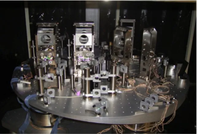
Figure 3.1: A picture taken of the setup for this work. The thermally insulated vacuum chamber that houses the two cavities is at the further end of the optical table.
3.1
Optical Cavity as a Frequency Reference
A Fabry–Perot cavity is formed by two reflecting mirrors facing each other, separated by a distance
L. One useful property of the Fabry–Perot cavity is frequency selection. Only light with certain frequencies can pass through the cavity. The cavity’s Free Spectral Range (FSR) frequencies are given by
ν=n c
2L, (3.1)
where n is an integer denoting the axial mode number. Basically, it is a condition that the laser must form a standing wave pattern in the cavity. This property allows a Fabry–Perot cavity be a useful tool for laser frequency stabilization. One important property of a laser is its highly coherence output, i.e., a single frequency light, but it has frequency noise which can be measured in the spectral density of noise power, Sν(f), inHz2/Hz or the linear spectral density, δν(f), with units
ofHz/√Hz.
The fundamental frequency noise in a laser is placed by the Schawlow-Townes limit [114,115],
SfS−T =δνL
r
2hν
Pout
(3.2)
whereδνL is the laser cold cavity line width andPout is the laser output power. This is the random
frequency noise from spontaneous emission inside a laser. The distribution is flat and can be as low as 0.5Hz/√Hz for 1mW output because of the narrow laser cavity linewidth [116]. However, the actual noise from a laser is far higher than this. Anything that changes the optical path length of the laser cavity affects the laser frequency. Frequency noise in a Non-Planar Ring Oscillator (NPRO) laser can be roughly estimated to be 10 kHz h1Hzf i√Hz
Hz from 1 Hz to 10 kHz. This estimated
frequency noise mostly originates from power fluctuations in its pump laser [117].
If the laser frequency is forced to follow the length of the cavity by means of frequency discrim-ination techniques e.g. Pound–Drever–Hall locking (PDH) [118, 119] (examples for comprehensive reviews of PDH technique can be found in Ref. [117, 120]). The laser frequency noise can be sup-pressed significantly until it matches the displacement noise of the reference cavity. The relation between the two is
δν
ν =−
δL
L . (3.3)
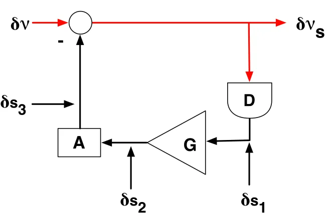
the loop is engaged, the suppressed frequency noiseδνs of the laser becomes
A
D
G
δ
ν
δ
L
-N
e
N
a
δ
ν
s
Figure 3.2: A block diagram of PDH lock. δν is the laser free running noise in Hz/√Hz, δνs is
the suppressed frequency noise, or the frequency noise of the transmitted beam behind the cavity,
δLis the cavity’s displacement noise which converts to the frequency noise via PDH lock. D is the frequency discriminator gain in V/Hz,Gis the servo gain in V/V,A is the actuator gain in Hz/V.
NeandNaare the error signal and the control signal, respectively. The minus sign from the actuator
A, represents the negative feedback. The minus sign fromδL means the displacement noise of the cavity is compared to the laser frequency.
δνs=
δν
1 +H + H
1 +H × c
LλδL (3.4a)
≈ δν
H +
c
LλδL for|H| 1. (3.4b)
Within the loop bandwidth, where the magnitude|H|of the open-loop gain is large, the displacement noiseδLof the cavity is impressed onto the frequency noise of the laser: δνs≈(c/Lλ)δL. The power
spectral density of the frequency noise is given bySν(f) =|δνs|2.
It is impossible to measureδLinside the control loop, asNeis an in-loop sensor,NAwill contain
only the information about the free running noise of the laser which is much larger than δL. To measure δL, we have to measure it optically from δνs as an out-of-loop witness. The transmitted
beam can be compared with a very stable reference, or beat against another identical setup. The latter method is chosen since it offers common mode rejections for disturbance from seismic noise, acoustic noise, ambient temperature noise, and other noises that are coherent between the two setups.
When directed onto an RF photodiode, the combined beam results in a beat note with frequency ˆ
ν =ν1−ν2 (the high frequency portionν1+ν2 is filtered out by a low pass filter). The frequency
noise of this beat note has a power spectral densitySνˆ=Sν1+Sν2 which can be read out using a
phase-locked loop (PLL) technique1which will be discussed in section4.6.
3.2
Prototype Setup
Instead of using two similar setups of a laser locked to a reference cavity as suggested at the beginning of this chapter, the first setup, serving as a prototype for thermal noise experiment, requires only one laser, one high performance frequency stabilizing servo (FSS), and two references cavities.
3.2.1
8–inch Reference Cavities
These referen
![Figure 1.1: Apparent power[V 2/R] vs. temperature, for Advance wire resistances [5]](https://thumb-us.123doks.com/thumbv2/123dok_us/954671.608657/11.612.188.464.325.543/figure-apparent-power-v-temperature-advance-wire-resistances.webp)
![Figure 1.4: Baseline Advanced LIGO’s noise budget (GWINC v2.0).125 W input power [43].Coating Brownian noise is plotted in confidence interval where uncertainties of coatings’ mechanicalloss angles and Young’s moduli are taken into consideration.](https://thumb-us.123doks.com/thumbv2/123dok_us/954671.608657/16.612.148.497.136.354/baseline-advanced-brownian-condence-interval-uncertainties-mechanicalloss-consideration.webp)