Complexity of Spectrum Activity and Benefits of
Reinforcement Learning for Dynamic Channel
Selection
Irene Macaluso, Danny Finn, Barıs¸ ¨
Ozg¨ul and Luiz A. DaSilva
Abstract—We explore the question ofwhenlearning improves the performance of opportunistic dynamic channel selection by characterizing the primary user (PU) activity using the concept of Lempel-Ziv complexity. We evaluate the effectiveness of a reinforcement learning algorithm by testing it with real spectrum occupancy data collected in the GSM, ISM, and DECT bands. Our results show that learning performance is highly correlated with the level of PU activity and the amount of structure in the use of spectrum. For low levels of PU activity and/or high complexity in its utilization of channels, reinforcement learning performs no better than simple random channel selection. We suggest that Lempel-Ziv complexity might be one of the features considered by a cognitive radio when deciding which channels to opportunistically explore.
Index Terms—Dynamic spectrum access, reinforcement learn-ing, Lempel-Ziv complexity.
I. INTRODUCTION
Learning has been a core idea in cognitive radio since its origin, as one of the steps in the cognition cycle proposed by Mitola. The intuition behind it is that by learning (about current uses of the spectrum, about channel conditions, even about a user’s intentions) a radio should be able to better navigate the increasingly complex wireless environment. In this paper, we explore the question ofwhenit is advantageous to bring the power of machine learning to bear on the problem of dynamic channel selection (DCS). In particular, we focus on the reinforcement learning (RL) paradigm, which allows agents to autonomously discover the mapping between situations and actions through a mechanism of trial and error. Machine learning performs sustained observation of an envi-ronment and task and identifies patterns in these observations. In applying RL to dynamic spectrum access (DSA) we must first determine whether the observable spectrum utilization contains enough structure, over an appropriate time scale, to be captured by a learning process. We must also ask ourselves whether RL is justified or whether simpler forms of adaptation suffice. Our objective is to answer these two questions relying on real traces of spectrum use.
Manuscript received Apr 12, 2012; revised Sep 1, 2012 and Nov 23, 2012. This material is based upon works supported by the Science Foundation Ireland under Grants No. 10/CE/I1853 and 10/IN.1/I3007.
I. Macaluso, D. Finn and L. DaSilva are with CTVR, Trinity College Dublin, Ireland (e-mail:[email protected], finnda,[email protected]). L. DaSilva is also with Virginia Tech, USA. Barıs¸ ¨Ozg¨ul contributed to this work while he was with CTVR, Trinity College Dublin, Ireland (e-mail: [email protected]). He is currently working at Xilinx, Dublin, Ireland. The authors gratefully acknowledge the use of wireless data from Spectrum Data Archive of the Institute of Networked Systems at RWTH Aachen University.
To study the first question above, we characterize the observability of spectrum utilization through the prism of Lempel-Ziv (LZ) complexity. To answer the second question, we compare the outcome of RL against the performance of a simple random channel selection scheme. We find out that, in a variety of frequency bands (namely, the 2.4 GHz ISM band, the DECT band, and the GSM900 and GSM1800 bands) the application of RL can be advantageous, but its performance benefits are highly correlated with the level of primary user (PU) activity observed and the amount of structure in these observations, estimated by the LZ complexity. In particular, our study shows that the LZ complexity of the PU’s behavior can account for up to a30%of difference in the probability of success of RL. This result does not just highlight the truism that the effectiveness of learning depends on the level of regularity of the PU activity. It also shows the importance of analyzing the performance of RL algorithms applied to DCS with respect to the complexity of the PU’s activity, a feature that has been overlooked in previous research in DSA. Our results show that the proposed measure of complexity is a theoretically sound and practical metric for predicting the effectiveness of RL for DCS. Moreover the same complexity measure plays a significant role in determining the impact of the number of observed channels on the RL performance.
The research presented in this paper can be situated within the broader perspective of the effectiveness of spectrum reuse mechanisms. This topic has been identified as an open research question in [1]. The primary contributions of this paper are to:
• Explore the effectiveness of reinforcement learning
ap-plied to dynamic channel selection, relying on actual spectrum measurement data;
• Determine the relationship between the effectiveness of
learning and the predictability of spectrum use by the PU, using the LZ complexity, both empirically and theoreti-cally; and
• Determine the relationship between the number of
ob-served channels, the performance of learning and the complexity of the PU’s activity.
of the bands by the PU. Section V presents the analysis of the impact of the number of observed channels on the performance of learning taking into account the complexity of the PU’s activity. Section VI describes the effect that the learned policy has on subsequent SUs attempting to access the same set of channels. We summarize our conclusions and point towards directions for future work in section VII.
II. RELATED WORK
In this paper we study the problem of dynamic channel selection in a vertical spectrum sharing environment. In oppor-tunistically occupying temporarily vacant channels, secondary users attempt to optimize their throughput whilst maintaining their level of interference to the primary user below a certain bound.
Machine learning has been widely applied to DSA [2], [3], [4]. Much of the previous analysis of the effectiveness of machine learning algorithms in DSA relies on simplified theoretical models of PU activity. In some cases, spectrum utilization from one instant in time to the next is assumed to be independent and identically distributed (i.i.d) [2], [3]. This assumption does not take into account the likely sequential patterns in the observations, and should be adopted only when either the analysis of the observed data confirms it or when the corresponding theoretical conditions are clearly satisfied.
In other works on DSA, the PU activity is often assumed to satisfy the Markov property [4], [5], [6]. A first order Markov model is often selected, as the parameter space increases exponentially with the order of the model. These models are mathematically tractable, but again it is important to validate their realism against actual measurement data. In our investigation, we rely instead on real spectrum data collected at RWTH Aachen [7] and by us at Trinity College Dublin (TCD).
There is some work in the cognitive radio literature that relies on empirical measurements to model channel activity. In [8] the authors make use of base station traffic logs collected by a GSM band network operator. Call arrival times and durations, as well as location-based patterns in network usage, were modeled. Here it was observed that the conventional modeling of call duration based on an exponential distribution did not apply. In [9] the authors used a traffic generator to load a WLAN and then characterized the resulting spectrum occu-pancy. In this case, it was found that a continuous-time semi-Markov model was effective in modeling idle periods between bursty transmissions. In [10] the authors verified the adherence to the Markov property for spectrum measurements collected in the paging band (928-948MHz). Most recently, the group at RWTH Aachen University [7], on whose measurements we rely, have derived stochastic models for PU duty cycle. These measurements consist of spectrum measurements of the
wireless environment in the range of20MHz to6GHz. In [11]
the authors used this dataset to validate the Beta distribution assumption for modeling channel occupancy. In [12] the au-thors used the RWTH Aachen dataset to study the effectiveness of opportunistic spectrum access mechanisms with and without knowledge of PU activity patterns. The authors observed how
the extracted spectrum, i.e. the effectiveness of the spectrum access mechanism, is only weakly related to the average spectrum availability. Our work, while confirming this result, moves one step further in proposing a metric to quantify the effects of different levels of regularity in spectrum usage on the performance of spectrum access mechanisms that are based on learning. In [13] we discussed the idea of using Lempel-Ziv complexity to recognise spectrum bands that present an opportunity to be exploited.
III. APPLICATION OFLEMPEL-ZIVCOMPLEXITY TO
PRIMARYUSERACTIVITY
Dynamic channel selection algorithms are usually charac-terized with respect to the duty cycle of the channels, i.e. they are evaluated with respect to the probability of the presence of PUs. Intuitively, the more activity PUs produce, the harder the DCS for SUs will be. However, when using machine learning, the traffic load is not sufficient to characterize the performance of a given DCS algorithm. In fact, the performance of a learning algorithm is influenced by the amount of structure in the data from which the algorithm is learning. In the particular case of an SU attempting to learn about the availability of channels, the success of the learning algorithm is affected by the amount of structure contained in the PU’s activity pattern. The more structured the data is, the more effective we can expect a learning algorithm to be. Therefore, measuring the amount of structure in channel availability, or its complexity, is of primary importance in assessing the usefulness of retaining past information to make better decisions in the future.
In this paper we quantitatively characterize the structure of a spectrum occupancy sequence by making use of a measure of complexity proposed by Lempel and Ziv [14]. In particular, we adopted the normalized Lempel-Ziv complexity, which measures the rate of production of new patterns in a sequence. Lempel and Ziv associated to every sequence a complexity
coefficient c which is computed by scanning the sequence
and incrementingcevery time a new substring of consecutive
symbols is found. Then c is normalized via the asymptotic
limit n/log2(n), wheren is the length of the sequence [15]. Lempel-Ziv complexity is a property of individual sequences and it can be computed without making any assumptions about the underlying process that generated the data. This feature is of the utmost importance when one is dealing with real data (in our case, sensed channel status in a variety of frequency bands). Furthermore, LZ complexity is strongly related to the source entropy. In fact, if the source is ergodic, the normalized LZ complexity has been proven [16] to be equal to the source entropy almost surely.
we conducted the same analysis using real spectrum occu-pancy data. We argue that the adopted measure of complexity provides an effective and new angle for analyzing the learning performance for DCS. Finally in section IV-C we presented a theoretical proof of the relationship between the entropy rate of the process that describes channel occupancy and the effectiveness of RL applied to DCS.
IV. ASTUDY ON THE EFFECTIVENESS OF
REINFORCEMENTLEARNING FORDCS
A learning algorithm applied to DCS aims at exploiting the spectrum occupancy history in order to make better decisions in the future. Reinforcement learning (RL) [17] has been one of the favorite choices for dynamic spectrum access applications [4], [6], [18]. In almost all cases, the performance of the proposed solutions has been studied with respect to PU activity levels. To the best of our knowledge, only [4] points out that the same PU activity level may result in different performance of RL, but the authors do not discuss what causes those differences. Below we will show that the effectiveness of an RL algorithm applied to DCS is strongly correlated with the LZ complexity of the sequence describing PU activity on the channels to be used opportunistically. Our
model considers a single SU that can use one of N
equal-bandwidth frequency channels opportunistically. Time is slot-ted and alternates between a sensing phase and a transmission phase. The SU is allowed to transmit in the time slot if the channel it selected in the sensing phase is still free. We consider a perfect sensing scenario where the local measures performed by the SU exactly represent the PU’s activity. The SU’s choice of which channel to attempt transmission in is made according to the policy determined by an RL algorithm. Full observability of the channels is assumed, and therefore, learning [19] is the most natural candidate. Moreover, as Q-learning does not require a model of the agent’s environment, it is suitable to deal with real spectrum occupancy data.
The goal of Q-learning is to find an optimal policy, i.e. the sequence of actions that maximizes the expected sum of discounted rewards. The agent state at timetis given byst= [X1,t, . . . , XN,t, ct], whereXi,t∈ {0,1}indicates whether the
ithchannel is free (0) or occupied (1) andct∈ {1, . . . , N}is the index of the channel the SU is accessing at timet. At time
t the SU performs an actionat∈ {1, . . . , N}, i.e. it selects a channelct+1. At timet+ 1it receives a rewardr(t+1)(st, at):
r(t+1)(st, at) = (1−Xat,t+1)−e(1at,ct) (1)
where1at,ct is0 ifat=ctand1 otherwise, ande∈[0,0.5].
In other words the SU is rewarded if it selects a free channel, while a cost of switching channels is also included to dis-courage too frequent channel changes. Based on the received reward, the agent updates the Q-values [19]:
Q(st, at) := Q(st, at) +αr(t+1)+
α(γmax at+1
Q(st+1, at+1)−Q(st, at)) (2) where0≤γ <1 is the discount factor andαis the learning rate. A value of γ different from 0 allows the agent to take into account the delayed reward when it selects an action.
In a stationary environment Q-learning is proven to converge to the optimal policy if α→ 0 and all the state-action pairs are visited an infinite number of times. During the learning stage, an exploration strategy is required to allow the agent to visit all the state-action pairs. A randomized strategy is commonly adopted: the agent selects a random action with a
probability and the best estimated action with probability
1 −. At the beginning the algorithm starts with a large
value of, which decreases as the Q-learning converges. For the experiments with the real spectrum occupancy data, the stationarity condition is generally not satisfied. Therefore we fix the learning factor to0.1to allow the agent to adapt to the changes in the environment. Moreover, in order to discover changes in the environment, the agent must be allowed to perform exploratory actions from time to time. Therefore we set the -value to 0.01. In the case of synthetic data, both
andαdecrease linearly with the time step.
A. Reinforcement Learning with Synthetic Data
Our goal here is to study the effect of both the levels of PU activity and the complexity of the PU behavior as defined in section III. To generate the synthetic data we modeled the
N channels as independent random variables. Each channel
is the realization of a 2−state first order Markov chain
(MC). Therefore we generated MCs with different values of stationary distribution and LZ complexity. For a homogeneous MC, the stationary distributionδsatisfies (3) and (4).
δ0=
1−p11 (1−p00) + (1−p11)
(3)
δ1=
1−p00
(1−p00) + (1−p11) (4)
whereP = p00p01
p10p11
is the transition probability matrix. As previously observed, for an ergodic source the Lempel-Ziv complexity equals the entropy rate of the source, which
for a Markov chainX is given by:
h(X) =−X ij
δipijlogpij. (5)
It is easy to verify that (3) and (4) constitute an undetermined system in the two unknownsp00 andp11corresponding to:
δ0p00+ (δ0−1)p11= 2δ0−1. (6) In principle we could fix the stationary distribution and the entropy rate and then compute the corresponding Markov tran-sition probability matrix using equations (5) and (6). However, the result will be a transcendental equation which is hard to solve. To sidestep this we fixed the stationary distributionδ0 and for each value of it we considered a range of values for eitherp11orp00and then we computed the correspondingp00
orp11. In other words, we calculated several entropy rates for
each value of the stationary distribution.
0.2 0.3 0.4 0.5 0.6 0.7 0.8 0.9 1 0.1
0.2 0.3 0.4 0.5 0.6 0.7 0.8 0.9 1
PRLsuc
pf
Average Lempel−Ziv Complexity
0.2 0.3 0.4 0.5 0.6 0.7 0.8 0.9
(a)
0.2 0.3 0.4 0.5 0.6 0.7 0.8 0.9 1
0.1 0.2 0.3 0.4 0.5 0.6 0.7 0.8 0.9 1
PRL
suc − P RCS suc
pf
Average Lempel−Ziv Complexity
0 0.05 0.1 0.15 0.2 0.25 0.3 0.35 0.4 0.45 0.5
(b)
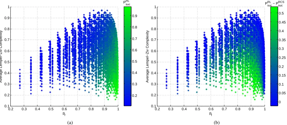
Fig. 1. (a) Probability of success of Q-learning as a function of the average LZ complexity and the probability of at least one free channel existing. Each point represents a particular instance of Q-learning applied toN = 3channels. The total number of possible combinations which we analyzed is 453= 14190. (b) Each point represents the difference between the probability of success of RL and the probability of success of the random channel selection approach applied to same ensemble of channels.
has been applied to all the possible combinations of N = 3
channels over the 45possible transition matrices.
Figure 1(a) shows the probability of success obtained by Q-learning as a function of the average entropy rate and the probabilitypf of at least one free channel existing, defined as:
pf = 1− N
Y
i=1
δ1,i (7)
whereδ1,i is the stationary distribution of theithchannel. Each point in the figure corresponds to one instance of
the RL problem. For each instance, we run 102 independent
simulations. For each simulation, first the optimal policy is computed using the Q-learning algorithm, then the resulting policy is evaluated over102 trials of104time steps each. For each trial the probability of success is computed according to the number of times that a free channel was selected over the length of the trial. Each point in Figure 1(a) represents the average of the results obtained for each of the104experiments.
As expected, the probability of success increases with pf.
However, it can be observed that the performance of RL is also strongly dependent on the complexity of the PU behaviors. For a certain value ofpf, the variation of the probability of success is up to 30%.
Figure 1(b) shows the difference between the probability
of success of RL (PRL
suc) and the probability of success
of a random channel selection (PRCS
suc ) approach. Although
RL always outperforms RCS, the difference in performance
becomes negligible not only when the pf is large, but also
when LZ complexity increases. Indeed it was to be expected that a random action selection algorithm is not influenced by the complexity of the PU behaviors. For a given pf, PsucRL
decreases when LZ complexity increases, while PsucRCS
re-mains almost constant. Therefore the performance gain of RL becomes less significant when LZ complexity increases. It is
worth noting that for a given LZ complexity, the performance gain of RL increases withpf up to a certain point; thereafter the performance of RCS approaches the performance of RL.
B. Reinforcement Learning with Measurement Data
In order to analyze whether the relationship between LZ complexity and the performance of RL for DCS also holds for real spectrum data, we relied on spectrum measurements conducted at RWTH Aachen [7], in frequency bands
rang-ing from 20 MHz to 6 GHz, and by us at TCD. The
RWTH Aachen measurements were recorded using an Agilent E4440A spectrum analyzer set to a resolution bandwidth of
200 kHz [7]. The measurements we recorded in TCD were
taken in the ISM band from 2.401 GHz to 2.433 GHz, in
an indoor location. These measurements were recorded using an Anritsu MS2721B handheld spectrum analyzer set to a
resolution bandwidth of200 KHz.
We considered a number of frequency bands: the 2.4 GHz ISM band, the DECT band, and the GSM900 and GSM1800 bands. For each band, Q-learning was applied to all the
possible combinations of N = 3 channels with duty cycle
DC ∈ [0.3,0.8]. In particular, we considered sequences of
spectrum occupancy over 12 hours (from 11:00 to 23:00)
for both the RWTH and the TCD datasets. Channels with a lower DC were not considered because the resulting DCS is unproblematic and even a random policy will exhibit nearly-optimal performance. On the other hand, channels with a too high DC were not considered because their exploitation will not result in a significant contribution for any kind of DCS approach. To convert the power spectral density estimates into
binary occupancy sequences we used a threshold of−107dBm
or −100 dBm for indoor and outdoor locations respectively,
[image:4.612.76.533.59.259.2](a) GSM900 (b) GSM1800 (c) DECT (d) ISM
Fig. 2. PU activity in indoor location across one day for various bands using a threshold of−107dBm.
0.75 0.8 0.85 0.9 0.95
0.45 0.5 0.55 0.6 0.65 0.7 0.75 0.8 0.85 0.9 0.95
pf
Average Lempel−Ziv Complexity
0.35 0.4 0.45 0.5 0.55 0.6 0.65 0.7 0.75 PRLsuc
(a)
0.76 0.78 0.8 0.82 0.84 0.86 0.88 0.9 0.92 0.94 0.45
0.5 0.55 0.6 0.65 0.7 0.75 0.8 0.85 0.9 0.95
pf
Average Lempel−Ziv Complexity
−0.05 0 0.05 0.1 0.15 0.2 0.25 0.3 P
suc RL
− P
suc Rand
(b)
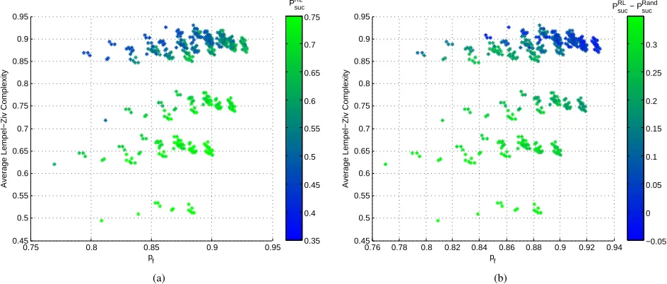
Fig. 3. ISM band (outdoor). (a) Probability of success of Q-learning as a function of the average LZ complexity and the probability of at least one free channel existing. Each point represents a particular instance of Q-learning applied to N = 3channels. The total number of possible combinations which we analyzed is 153= 455, where15is the number of channels withDC∈[0.3,0.8]. (b) Each point represents the difference between the probability of success of RL and the probability of success of the random channel selection approach applied to same ensemble of channels.
GSM 900, GSM 1800, DECT and ISM 2.4 GHz frequency
bands. The DC is displayed for sampled time periods of1000
samples, equivalent to roughly 30minutes.
Each combination of channels corresponds to one instance of the RL problem. For each instance, we run103independent simulations. For each simulation, first the optimal policy is computed using the Q-learning algorithm considering only the first hour of the sequences of spectrum occupancy, then the resulting policy is evaluated over the remaining11hours. For each simulation the probability of success is computed according to the number of times that a free channel was selected over the length of the spectrum occupancy sequences. The probability of success of each RL instance is the average
over the 103 simulations. Analogously, the probability of
success of a random channel selection (PRand
suc ) approach is
computed as the number of times that a free channel was selected by the random channel selection (RCS) scheme over the length of the spectrum occupancy sequences, averaged over 105 simulations. Figures 3(a) and 4(a) show the probability of success obtained by Q-learning as a function of LZ complexity andpffor all the possible combinations of channels in the ISM band and the GSM1800 bands respectively. The probabilitypf
is computed according to (7), where the duty cycle of each channel is used as an estimate of the stationary distribution. The LZ complexity of each channel is computed using the algorithm described in [15], while the average value is used as an approximation of the complexity of each combination of channels.
For the ISM band (see Figure 3(a) and 3(b)), the values for the average LZ complexity span a considerable range and
we can easily observe that, when pf remains constant, the
RL performance decreases when LZ complexity increases. Moreover the difference in performance between RL and RCS
is up to 30% when the average LZ complexity is low. This
is consistent with the results shown for synthetic data. It
should be noted that both the average LZ complexity andpf
do not cover the same range for each band. For example, for the DECT band, the average LZ complexity is always greater than 0.93. Accordingly, the PsucRL is only moderate, and the difference in performance between RL and RCS is
never greater than 10%. The GSM900 and GSM1800 bands
present intermediate values of average LZ complexity and
PRL
suc correspondingly. It can be observed in Figure 4(a) that in
the case of the GSM1800 band thePRL
[image:5.612.71.543.212.413.2]0.65 0.7 0.75 0.8 0.85 0.9 0.95 1 0.75
0.8 0.85 0.9 0.95 1
pf
Average Lempel−Ziv Complexity
0.35 0.4 0.45 0.5 0.55 0.6 0.65 0.7 0.75 PRLsuc
(a)
0.65 0.7 0.75 0.8 0.85 0.9 0.95 1
0.75 0.8 0.85 0.9 0.95 1
pf
Average Lempel−Ziv Complexity
−0.05 0 0.05 0.1 0.15 0.2 0.25 0.3 PsucRL − PsucRand
[image:6.612.71.544.55.257.2](b)
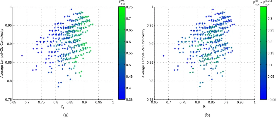
Fig. 4. GSM1800 band (outdoor). (a) Probability of success of Q-learning as a function of the average LZ complexity and the probability of at least one free channel existing. Each point represents a particular instance of Q-learning applied toN= 3channels. The total number of possible combinations which we analyzed is 143= 364, where14is the number of channels withDC∈[0.3,0.8]. (b) Each point represents the difference between the probability of success of RL and the probability of success of the random channel selection approach applied to same ensemble of channels.
70%. The performance in the ISM band is on average better only because the ISM channels exhibit a more structured, i.e. less complex, activity. On the other hand the DC values, and therefore thepf values, span almost the same range of values
for both the ISM band and the GSM1800 band. As thePRand
suc is not affected by the complexity of the PU behavior, but it only depends on the probability of the presence of PUs, this explains the negligible difference between the learned policy and the random policy in the case of the GSM1800 band. The data collected by us at TCD exhibits a significantly lower LZ complexity than the measurements taken in Aachen. Nonetheless, the performance of RL, as well as the difference in performance with respect to RCS, is consistent to what we observed for the Aachen dataset. It should be noted that we cannot draw conclusions aimed at characterizing the PU’s behavior in the various bands. Indeed the same band in different locations and/or using different sensing techniques may exhibit different values of complexity, as demonstrated by the ISM band in our analysis. In any case, all the frequency bands examined by us exhibit the same kind of relationship
between average LZ complexity, pf and the performances of
RL and RCS, confirming that the LZ complexity is a valid metric for the analysis of learning performance.
For given values of LZ complexity andpf, the performance of RL for real spectrum data is usually lower than the corresponding performance for synthetic data. This can be explained by considering two factors. Although Q-learning does not require a model of the agent’s environment, the underlying assumption is that the environment satisfies the Markov property. To verify whether the Markov property holds, we compared the sample autocorrelation function of the binary spectrum occupancy of a channel and the theoretical autocorrelation function of the corresponding (estimated) 2-state first order Markov chain. To remove the probable non-stationarity effects, we considered a sufficiently small analysis
window of two hours for the estimation of both the sample autocorrelation and the Markov chain. For almost all the spectrum occupancy sequences it can be observed that, as the lag increases, the sample autocorrelation deviates significantly from the theoretical one. Moreover, due to the nonstationarity
of the spectrum data, both the learning factor α and the
exploration coefficient do not converge to zero. This way,
Q-learning is able to track the changes in the environment; the cost to be paid is a certain amount of inefficiency due to the necessary random exploration the algorithm has to perform.
C. Theoretical analysis
In this section we conduct a theoretical study of the relationship between the entropy rate of the Markov chain that models the PU’s behavior and the performance of RL, which confirms our empirical findings. Let us denote by
E∗[r] the expected reward of an SU that selects a channel according to the optimal policy estimated by Q-learning using the reinforcement scheme in (1).
Theorem 1. If each of the N channels is the realization of a 2−state first order Markov chain p00 1−p00
1−p11 p11
and the discount factor γ = 0, for any given stationary distribution
[δ0, δ1] of the Markov chain, thearg max of the entropy rate
of the Markov chain is one of the points for whichE∗[r]has a global minimum (when the cost of switching channelse ∈
(0,0.5)).
Proof: For any given stationary distribution, the entropy
rate has a unique global maximum at p00 =δ0. This can be
verified by expressing the entropy rate as a function of p00 using (3) and then writing its first derivative with respect to
p00:
dh dp00
=−δ0
log2
p00
1−p00
+ log2
2δ0−1−δ0p00 δ0(p00−1)
.
E∗[r] =
δ0Np00+δN1 (1−p11) +N1
NX−1
n=1
N!δn
1δ
N−n
0 ((N−n)p00+n(p00−e))
n!(N−n)! ifp00≥δ0+eδ1
δ0Np00+δN1 (1−p11) +N1
NX−1
n=1
N!δn
1δN0−n((N−n)(1−p11−e) +n(1−p11))
n!(N−n)! ifp00≤δ0−eδ1
δN
0 p00+δN1 (1−p11) +N1
NX−1
n=1
N!δn
1δN0−n((N−n)p00+n(1−p11))
n!(N−n)! ifp00∈[δ0−eδ1, δ0+eδ1] (9)
dE∗[r]
dp00 =
1−δN1−1 ifp00≥δ0+eδ1
δ0(δ0N−1−1)
1−δ0
ifp00≤δ0−eδ1
δN0 −δ
N−1
1 δ0+N1
NX−1
n=1
N!δn
1δN0−n n!(N−n−1)!−
N!δn−1 1 δ
N−n+1
0
(n−1)!(N−n)!
ifp00∈[δ0−eδ1, δ0+eδ1]
(10)
E∗[r] =
δN0 p00+δ1N(1−p11) +
NX−1
n=1
N!δn
1δ
N−n
0
n!(N−n)!p00 ifp00≥δ0
δN
0 p00+δ1N(1−p11) +
NX−1
n=1
N!δn
1δN0−n
n!(N−n)!(1−p11) ifp00< δ0
(11)
Under the assumption of independence between channels and identical Markov transition probability matrices, the expected reward of an SU can be written as in (9). By expressing p11 as a function of p00 using (3), it can be verified that (9) is a continuous function of p00, for any given δ0. After some manipulations, the first derivative of (9) is given by (10).
It is easy to verify that, if δ0 ∈ [0,1], the first equation in (10) is positive, the second equation in (10) is negative, and the third equation in (10) is null. All the points p00 ∈ [δ0−eδ1, δ0+eδ1]correspond to global minima of the expected reward. As δ0 ∈ [δ0 −eδ1, δ0 +eδ1], the optimal expected reward has a global minimum at p00=δ0.
Corollary 1. Ife= 0and γ= 0,E∗[r] has a unique global minimum at p00=δ0.
Proof:In this case the optimal expected reward simplifies in (11) which has a unique global minimum at p00=δ0.
The maximum of the entropy rate, which coincides with the LZ complexity for an ergodic source, and the minimum of the optimal expected reward occur for the same value p00 =δ0, confirming the relationship between the LZ complexity and the Q-learning performance.
Although the theoretical analysis presented in this section applies only to myopic agents, i.e. agents that only seek to
maximize the immediate reward (γ = 0), it should be noted
that the results shown in the figures in Section IV refer to
γ= 0.9. Moreover, we run the same experiments discussed in sections IV-A and IV-B using a range of values for γand the results always exhibit the same kind of relationship between
average LZ complexity, pf and the performance of RL.
D. Predicting RL performance for DCS
In the previous sections we analyzed the performance of RL with respect to two features, namely the DC - expressed in terms of pf - and the LZ complexity of a set of channels.
We now turn our attention to using these two features in a proactive way and we show that a cognitive radio can predict the probability of success of RL given the DC and LZ complexity of a set of observed channels, and hence decide whether to adopt RL for DCS.
No definite black-and-white boundary can be given to separate situations, i.e. channel activities, where learning is advantageous from situations where it is not, as this boundary depends on the SU’s requirements. However, if we assume that the SU’s requirements can be expressed in terms of the probability of success of accessing a free channel, it is possible to exploit the results discussed above to design a procedure that allows a cognitive radio to make such decision.
In the remainder of this section we assume that an SU can
observe N = 3 channels and can estimate the corresponding
LZ complexity and DC values. Predicting the PsucRL given
the DC and the LZ complexity of a set of channels can be cast as a regression problem, which we addressed by using a feed-forward neural network with a single hidden layer of 10units. We trained the network over the dataset described in Section IV-A using the Levenberg-Marquardt algorithm [20]. We used70%of the14190channels sets as training data,15% as validation data, and the remaining15%as test data (test set 1). The inputs to the network are the DC and LZ complexity
values of the 3 channels; the output is the corresponding
PRL
suc. Moreover, to further test the prediction accuracy of
the network, we generated additional MCs corresponding to stationary distributions not included in the dataset described
in Section IV-A. We considered 8 additional possible δ0
values in the range 0.15,0.25, . . . ,0.85. For each of these values, we consideredp11 (orp00) values of0.2,0.4,0.6,0.8 if δ0 >= 0.5 (if δ0 <0.5), obtaining 32 different transition probability matrices. Finally Q-learning has been applied to
all the possible combinations of N = 3 channels over the
0 500 1000 1500 2000 2500
Instances
Errors
−0.065 −0.055 −0.045 −0.035 −0.025 −0.015 −0.005 0.005 0.015 0.025 0.035 0.045 0.055
[image:8.612.62.292.51.224.2]Test set 2 Test set 1 Zero Error
Fig. 5. Histogram of the error values. The error is computed as the difference between the actualPsucRLand the output of the network.
channels sets and their corresponding PRL
suc, estimated by
averaging the results of 102 independent simulations, were
used to test the network accuracy (test set2).
Figure 5 shows the histogram of the error values, where the error is the difference between the actualPsucRLand the output of the network. It can be observed that the prediction accuracy of the neural network is extremely high. Indeed in93%of the instances the difference between the network output and the
PRL
suc is less than 2.5% for both test sets. This result shows that the neural network is able to accurately predict thePRL suc even when presented with channels exhibiting new values of stationary distributions and complexity. Hence, an SU can reliably decide whether to adopt RL for DCS by comparing the predicted PRL
suc with its minimum required performance.
V. ON THE IMPACT OF THE NUMBER OF OBSERVED CHANNELS ON THERLPERFORMANCE
In this section we analyse the impact the numberN of chan-nels that the cognitive radio observes has on the performance
of RL. We will also analyse the relationship between N and
the entropy rate.
Theorem 2. If each of the N channels is the realization of a 2−state first order Markov chain p00 1−p00
1−p11 p11
and the discount factor γ = 0, for any given stationary distribution
[δ0, δ1]of the Markov chain, then theE∗[r]does not decrease
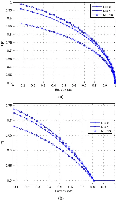
with N (when the cost of switching channelse∈(0.0,1.0)). The increment ofE∗[r]is either null or it decreases exponen-tially withN.
Corollary 2. Ife= 0andγ= 0,E∗[r]increases with N and its increment decreases exponentially withN.
The proofs can be found in the Appendix.
The most interesting aspect of the above result is that the performance improvement that a cognitive radio can achieve by increasing the number of sensed channels exponentially decreases to zero. This result has at least two important con-sequences. First, limiting the number of channels a cognitive radio observes impacts the amount of resources devoted to the sensing stage. For example, this implies the possibility
0 0.1 0.2 0.3 0.4 0.5 0.6 0.7 0.8 0.9 1
0.5 0.55 0.6 0.65 0.7 0.75 0.8 0.85 0.9 0.95 1
Entropy rate
E[r*]
N = 3 N = 5 N = 10
(a)
0.1 0.2 0.3 0.4 0.5 0.6 0.7 0.8 0.9 1
0.5 0.55 0.6 0.65 0.7 0.75
Entropy rate
E[r*]
N = 3 N = 5 N = 10
[image:8.612.334.528.52.389.2](b)
Fig. 6. (a) Optimal expected reward as a function of the entropy rate and the number of channelsN with no cost of switching (e= 0). (b) Optimal expected reward as a function of the entropy rate and the number of channels
Nwithe= 0.5.
of using less sophisticated hardware in the radio front-end as well as a reduction of the energy consumption of the sensing stage. Second, a reduced cardinality of the action space and the state space (N andN2N respectively, assuming a not null cost of switching channel) results in a faster convergence of the learning algorithm.
entropy rate is formalized in the following theorem, whose proof is given in the Appendix.
Theorem 3. If each of the N channels is the realization of a 2−state first order Markov chain p00 1−p00
1−p11 p11
and the discount factor γ = 0, for any given stationary distribution
[δ0, δ1] of the Markov chain and for any N, the arg max of
the entropy rate of the Markov chain is one of the points for which the ∆E∗[rN] has a global minimum (when the cost of
switching channels e∈[0.0,1.0)).
VI. ON THE IMPACT OFRLON SUBSEQUENT CHANNELS
EXPLOITATION
The analysis discussed in this section focuses on a scenario where multiple SUs are operating, but they do not simulta-neously start the learning process. In particular, an additional SU becomes active only after previous SUs have reached a stationary policy. This way, the problem we address remains in the domain of single-agent RL.
Multi-agent RL (MARL) evolved from the single-agent setting. One possibility that has been widely investigated [21] is that of ”independent Q-learning”, where each agent uses the traditional Q-learning algorithm while ignoring the presence of the other agents acting in the same environment and con-sidering the results of this interaction as noise. However, the convergence result no longer holds due to the non-stationarity of the environment caused by the dynamics of the other agents operating in the same environment. As a result, in some cases the agents may exhibit cyclic behavior. Various attempts have been made to find a different paradigm for MARL. In particular, the MARL problem has been modeled as a stochastic game. The reader is referred to [22] for an example of such approaches. A common issue with many of these approaches is that a coordination mechanism is required for all but a restricted class of games where all the agents achieve the maximum expected return in correspondence to the same Nash equilibrium.
A number of MARL algorithms have also been proposed that can only deal with repeated stateless games (see [21] and references therein). In the CR literature independent Q-learning has also been used in this fashion [23]. In the case of repeated games, other RL schemes, such as learning automata [24], can also be adopted. A learning automaton is a reinforcement learning scheme where each agent directly updates its action probabilities based on the environment response. We have recently applied learning automata to the problem of distributed channel selection in a cognitive radio network in the context of frequency-agile radios that are able to operate in multiple frequency bands simultaneously [25]. We formulated the problem as an N-player stochastic game and we proved that, by adopting learning automata, radios will converge to a Nash equilibrium, under the assumption of symmetric interference between the players.
In the remainder of this section we focus our attention on how the policy learned by the SU affects the channels’ char-acteristics. This in turn affects the performance of subsequent SUs trying to access the same set of channels.
We considered a number of combinations of N = 3
channels characterized by the same level of PU activity (δ0 = 0.5) and a range of values of entropy rate. For each combination of channels we run102independent simulations. As in section IV-A, first the optimal policy is computed, then the learned policy is evaluated over102trials of104time steps each. The resulting sequences of spectrum occupancyXi,t of
a channeliare then used to compute the maximum likelihood
estimate of the transition probability matrix of a first order Markov model. The estimated MCs summarize the activity on the channels of both the PUs and the SU. For each set of channels an additional SU has been trained using the estimated MCs to model the channels activity. This means that, from the additional SU’s point of view, there’s no difference between dealing with PUs and SUs or PUs only: it has to learn to select a channel that is free from both PU’s and other SU’s activity.
0.2 0.3 0.4 0.5 0.6 0.7 0.8 0.9 1
0.4 0.5 0.6 0.7 0.8 0.9 1
pf
[image:9.612.325.538.259.426.2]Average Lempel−Ziv Complexity
Fig. 7. Evolution of the channels’ characteristics in the LZ-pf plane. Each
circle corresponds to one combination of channels used only by PUs. Asterisks denote the LZ complexity and thepfof a set of channels when an SU executes
the learned policy. Finally, squares correspond to the channels’ characteristics observed when the PUs and both SUs are active.
Figure 7 represents the evolution of the LZ complexity and thepf of various combination of channels in correspondence to the activity of PUs only, PUs and one SU, PUs and two SUs. Each circle in Figure 7 corresponds to one combination
of 3 channels used only by PUs. Since all the channels are
initially characterized by the same level of PU activity, all the combinations correspond to the same value ofpf = 0.875. By construction they exhibit a range of values for the complexity. The combined activity of the PUs and of an SU executing the learned optimal policy is shown in Figure 7 by the asterisks. Each set of channels shows a decreased value of pf. In par-ticular, according to the results presented in previous sections, the lower the initial complexity, the lower the resultingpf, i.e. the higher thePsucRL.
The complexity of the channel activity resulting from the combined exploitation shows a narrower range of values with respect to the initial values. This can be explained by considering that the range of values allowed for the entropy rate depends on the stationary distribution of the MC (i.e. the
E∗[r] =E∗[rN] =
p00−δN1(p00−1 +p11)−Ne
NX−1
n=1
nN!δ
n
1δ
N−n
0
n!(N−n)! ifp00≥δ0+eδ1
1−p11−δ0N(−p00+ 1−p11)−Ne
NX−1
n=1
N!δn
1δN0−n(N−n)
n!(N−n)! ifp00≤δ0−eδ1
p00−δN1(p00−1 +p11) +N1
NX−1
n=1
nN!δ
n
1δN0−n(1−p00−p11)
n!(N−n)! ifp00∈[δ0−eδ1, δ0+eδ1]
(12)
The squares in Figure 7 correspond to the combined activity of the PUs, an SU executing the policy learned to coexist with the PUs, and an additional SU performing the policy learned to coexist with the PUs and the former SU.
As expected, the PRL
suc of the additional SU decreases, in
accordance with the lower values ofpf. The most interesting aspect of the above results is that the complexity values overall decrease as the exploitation of the channels increase, i.e. when more SUs start using the channels.
VII. CONCLUSIONS ANDFUTUREWORK
While the adoption of learning algorithms is often assumed to be beneficial to SUs seeking to use channels opportunis-tically, in this paper we show that these benefits depend strongly on the pattern of utilization of channels by the
PU. For this purpose, four frequency bands (ISM 2.4 GHz,
GSM900, GSM1800, and DECT) are taken into account, and we show that RL is beneficial, but only for some levels of PU activity and complexity. Although the regularities of the channels’ utilization doubtlessly influence the performance of learning for DCS, this aspect has not been investigated in previous research in DSA. Our study shows that the LZ complexity is a valid measure to quantify those regularities both for experimental utilization data and for data generated by idealized mathematical models of PU activity.
We suggest that the same approach can also be used by cognitive radios in a proactive way and our study shows that a cognitive radio could use LZ complexity to decide whether learning is the appropriate tool to utilize in a given situation. In this respect, we are currently investigating the usage of the LZ complexity as a feature that a cognitive radio could employ to focus its resources on a subset of channels that exhibit a more structured pattern of activity. No definite black-and-white boundary can be given to separate situations, i.e. channel activity, where learning is advantageous from situations where it is not, as this boundary depends on the SU’s requirements. Consider, for example, an SU that is connected to a machine-to-machine application and assume that it can attempt to opportunistically exploit a set of channels each exhibiting a
DC= 0.5 and high values of complexity. As this type of
SU can adjust its traffic schedule to suit the variances in a given band, it might be sufficient in this case to exploit only one channel, i.e. obtaining a Psuc = 0.5, without employing any learning technique. However, for a different SU connected to a time-sensitive application the same value of Psuc could be insufficient and even the small improvement provided by RL in correspondence to high values of complexity would be considered necessary.
APPENDIX
A. Theorem 2
Proof: After some manipulations, the optimal expected reward in (9) can be written as in (12) at the top of the page, where the notation makes explicit the dependence ofE∗[r]on
the number of observed channelsN.
By exploiting the binomial theorem, the first equation in (12) simplifies to:
p00−δN1 (p00−1 +p11)− e N
NX−1
n=1
nN!δ
n
1δN0−n n!(N−n)!
= p00−δN1 (p00−1 +p11)−eδ1
NX−1
n=1
N−1
n−1 !
δn1−1δ
N−n
0
= p00−δ1N(p00−1 +p11)−eδ1(1−δN1−1)
(13)
By analogous manipulations of the second and third equa-tion in (12), we can write the variaequa-tion of the optimal expected reward with respect toN as:
∆E∗[rN] =
δ0δ1N(p11+p00−1−e) ifp00≥δ0+eδ1 δ1δ0N(1−e−p00−p11) ifp00≤δ0−eδ1
0 otherwise
(14) The first and second equation in (14) are always positive
and exponentially decreasing withN.
B. Corollary 2
Proof:In this case, ∆E∗[rN]simplifies to:
∆E∗[rN] =
δN1 (1−δ1)(p11+p00−1) ifp00≥δ0 δN0 (1−δ0)(1−p00−p11) ifp00≤δ0
(15)
which is always positive and exponentially decreasing withN.
C. Theorem 3
Proof:By expressing p11 as a function ofp00 using (3), it can be verified that (14) is a continuous function ofp00, for any givenδ0and for any N. We can write the first derivative of (14) as:
d∆E∗[rN]
dp00
=
δN1−1(1−δ1) ifp00≥δ0+eδ1 −δN
0 ifp00≤δ0−eδ1
0 ifp00∈[δ0−eδ1, δ0+eδ1]
As the first, second and third equations in (16) are positive, negative and null respectively, all the points p00 ∈ [δ0 −
eδ1, δ0+eδ1]correspond to global minima of the increment of the expected reward. Asδ0∈[δ0−eδ1, δ0+eδ1], the∆E∗[rN] has a global minimum atp00=δ0.
REFERENCES
[1] C. Partridge, “Forty data communications research questions,” ACM SIGCOMM Computer Communication Review, vol. 41, no. 5, pp. 24–35, 2011.
[2] U. Berthold, F. Fu, M. van der Schaar, and F. Jondral, “Detection of spectral resources in cognitive radios using reinforcement learning,” in 3rd IEEE Symposium on New Frontiers in Dynamic Spectrum Access Networks, 2008.
[3] L. Lai, H. El Gamal, H. Jiang, and H. Poor, “Cognitive medium access: Exploration, exploitation and competition,”IEEE/ACM Trans. on Networking, 2007.
[4] W. Zhao, L. Tong, A. Swami, and Y. Chen, “Decentralized cognitive MAC for opportunistic spectrum access in ad hoc networks: A POMDP framework,” IEEE Journal on Selected Areas in Communications, vol. 25, no. 3, p. 589, 2007.
[5] A. Motamedi and A. Bahai, “Optimal channel selection for spectrum-agile low-power wireless packet switched networks in unlicensed band,” EURASIP Journal on Wireless Communications and Networking, vol. 2008, pp. 1–10, 2008.
[6] J. Unnikrishnan and V. Veeravalli, “Algorithms for dynamic spectrum access with learning for cognitive radio,”IEEE Transactions on Signal Processing, vol. 58, no. 2, pp. 750–760, 2010.
[7] M. Wellens, J. Riihij¨arvi, and P. M¨ah¨onen, “Empirical time and fre-quency domain models of spectrum use,” Physical Communication, vol. 2, no. 1-2, pp. 10–32, 2009.
[8] D. Willkomm, S. Machiraju, J. Bolot, and A. Wolisz, “Primary user behavior in cellular networks and implications for dynamic spectrum access,”IEEE Communications Magazine, vol. 47, no. 3, pp. 88–95, 2009.
[9] S. Geirhofer, L. Tong, and B. Sadler, “A measurement-based model for dynamic spectrum access in WLAN channels,” inProc. IEEE MILCOM. Citeseer, 2006.
[10] C. Ghosh, C. Cordeiro, D. Agrawal, and M. Rao, “Markov chain existence and hidden markov models in spectrum sensing,” inPervasive Computing and Communications, 2009. PerCom 2009. IEEE Interna-tional Conference on. IEEE, 2009, pp. 1–6.
[11] C. Ghosh, S. Roy, and M. Rao, “Modeling and validation of channel idleness and spectrum availability for cognitive networks,”IEEE Journal on Selected Areas in Communications, vol. 30, no. 10, pp. 2029–2039, 2012.
[12] V. Kone, L. Yang, X. Yang, B. Zhao, and H. Zheng, “On the feasibility of effective opportunistic spectrum access,” inProceedings of the 10th annual conference on Internet measurement. ACM, 2010, pp. 151–164. [13] I. Macaluso, T. Forde, L. DaSilva, and L. Doyle, “Impact of cognitive radio: Recognition and informed exploitation of grey spectrum opportu-nities,”Vehicular Technology Magazine, IEEE, vol. 7, no. 2, pp. 85–90, 2012.
[14] A. Lempel and J. Ziv, “On the complexity of finite sequences,”IEEE Transactions on Information Theory, vol. 22, no. 1, pp. 75–81, 1976. [15] F. Kaspar and H. Schuster, “Easily calculable measure for the complexity
of spatiotemporal patterns,”Physical Review A, vol. 36, no. 2, pp. 842– 848, 1987.
[16] J. Ziv, “Coding theorems for individual sequences,”IEEE Transactions on Information Theory, vol. 24, no. 4, pp. 405–412, 1978.
[17] R. Sutton and A. Barto,Reinforcement learning: An introduction. The MIT press, 1998.
[18] K. Yau, P. Komisarczuk, and P. Teal, “Applications of Reinforcement Learning to Cognitive Radio Networks,” in 2010 IEEE International Conference on Communications Workshops (ICC). IEEE, 2010, pp. 1–6.
[19] C. Watkins and P. Dayan, “Q-learning,”Machine learning, vol. 8, no. 3, pp. 279–292, 1992.
[20] M. Hagan, H. Demuth, and M. Beale, “Neural network design,” 1996. [21] L. Busoniu, R. Babuska, and B. De Schutter, “A comprehensive survey
of multiagent reinforcement learning,”Systems, Man, and Cybernetics, Part C: Applications and Reviews, IEEE Transactions on, vol. 38, no. 2, pp. 156–172, 2008.
[22] M. Bowling and M. Veloso, “An analysis of stochastic game theory for multiagent reinforcement learning. cmu-cs 00-165,” 2000.
[23] K. Yau, P. Komisarczuk, and P. Teal, “Performance analysis of reinforce-ment learning for achieving context awareness and intelligence in mobile cognitive radio networks,” in Advanced Information Networking and Applications (AINA), 2011 IEEE International Conference on. IEEE, 2011, pp. 1–8.
[24] K. Narendra and M. Thathachar,Learning automata: an introduction. Prentice-Hall, Inc., 1989.
[25] I. Macaluso, L. DaSilva, and L. Doyle, “Learning Nash Equilibria in Distributed Channel Selection for Frequency-agile Radios,” in ECAI 2012 Workshop on Artificial Intelligence for Telecommunications and Sensor Networks, 2012.
Irene Macaluso is a Research Fellow at CTVR -The Telecommunications Research Centre based at Trinity College, Dublin. Dr. Macaluso received her Ph.D. in Robotics from the University of Palermo in 2007. Dr. Macaluso’s current research interests are in the area of cognitive radio networks, with particular focus on the application of machine learning to wireless resource management and reconfigurable wireless networks.
Danny Finnreceived B.A. (Mathematics) and B.A.I. (Engineering) degrees from Trinity College Dublin in 2010 where he is currently a Ph.D. candidate with CTVR / The Telecommunications Research Centre. He is a key member of CREW - an FP7 project focusing on the creation of a federated test platform for advanced spectrum sensing and cognitive radio technologies. His research interests include cellular and cognitive radio network optimisation, and ad-vanced physical layer adaptations.
Barıs¸ ¨Ozg ¨ul received the B.S., M.S., and Ph.D. degrees in electrical and electronics engineering from Boˇgazic¸i University, ˙Istanbul, Turkey, in 1998, 2002, and 2008, respectively. From 1998 to 2003, he worked in Nortel Netas¸ as a R&D engineer and soft-ware architect. He joined Turkcell in 2003, where he worked as an expert in the network platform development team until June, 2005. From June 2005 to March 2008, he was a member of the Wire-less Communications Laboratory (WCL) at Boˇgazic¸i University. From May 2006 to November 2006, he was a visiting researcher in the Wireless Systems Laboratory (WSL), Georgia Institute of Technology. In 2008 he joined CTVR, The Telecommunications Research Centre in Trinity College Dublin, where he worked as a postdoctoral researcher focusing on next generation wireless networks. Since September 2011, he has been working as a research scientist at Xilinx, Dublin, Ireland.