An Analysis of Low Complexity Algorithms
for MIMO Antenna Selection
Peter J. Smith
†Tim W. King
†Lee M. Garth
†Mischa Dohler
∗† Department of Electrical and Computer Engineering, University of Canterbury, Christchurch, New Zealand
Email:{p.smith,twk20,l.garth}@elec.canterbury.ac.nz
∗ France T´el´ecom R&D, 28 Chemin du Vieux Chˆene, 38243 Meylan Cedex, France
Email: [email protected]
Abstract— In this paper we consider transmit and receive selection methods designed to achieve high channel capacities in a single-user MIMO link. A variety of radio channels are considered, including i.i.d. Rayleigh, correlated Rayleigh and Ricean fading environments. Also considered is the presence of imperfect channel state information (CSI) and a simplified waterfilling scheme. In all cases, we evaluate the performance of optimal selection, simple norm based selection and other benchmark selection techniques. The major contribution is a general approach to analyzing the capacity of the selection schemes via a simple power scaling factor. We are able to assess the impact of different channels, imperfect CSI and power allocation using this power scaling factor. Furthermore, the analysis is valid for all scenarios: transmit selection, receive selection and joint transmit-receive selection. Results are shown which compare the capacity performance over a wide range of cases. A notable conclusion is that optimal selection, which is computationally intensive, is outperformed at low SNR by the simple, norm based approach with power allocation.
I. INTRODUCTION
Given the advantages of wireless Input Multiple-Output (MIMO) systems, using transmit (TX) and receive (RX) antenna arrays, much attention has been paid to these systems and their potential limits. As the system sizes are increased to utilize the potential of MIMO techniques, the increased hardware requirements become a key issue. Multiple RF chains are needed to optimize performance at the expense of cost and volume. In this paper we consider a simple yet powerful approach for reducing the system complexity whilst retaining a considerable portion of the increased rates from using MIMO technology. Using the principle of antenna selection at the TX and/or RX side, RF chains can be optimally assigned to a subset of the available antennas. This provides greater spatial multiplexing gain without a large increase in the system’s hardware needs.
Many researchers have proposed algorithms for antenna selection [1]–[3]. Some of these approaches focus on selection to minimize outage probabilities or error rates [4], [5]. We con-sider selection methods which target high capacity values as in [2], [6]. Previous work in this area includes simple methods [1], [3], [7], variants of which are discussed in this paper, as well as complex methods [8], which may give slightly better performance than the simple methods but with much greater computational complexity. In this paper we propose to build on the ideas in [1]–[3], analyzing and extending the algorithms
that were discussed. We demonstrate in our statistical analysis of the resulting channel capacities that the selection process can be modeled as a simple scaling of the SNR, resulting in a performance gain. Thus, we propose the SNR scaling factor as a very simple metric which can be used to compare the performances of the algorithms. Note that this approach is extremely general and can be used for a variety of channels, selection scenarios, and also when channel estimation errors are considered.
This paper is organized as follows. In Sec. II we review the MIMO channel model, the channel capacity for antenna selection systems and a model for imperfect channel state in-formation (CSI). We introduce our various selection algorithms in Sec. III, followed by a statistical analysis of the algorithms in Sec. IV. Then we explore the effects of imperfect channel knowledge in Sec. V. We verify our analysis using Monte Carlo simulations in Sec. VI. We conclude in Sec. VII.
II. MIMO CHANNELMODEL ANDCAPACITY
We focus on a single user MIMO link withn transmitters
andmreceivers with channel observations of the form
r=Hu+n (1)
where vectorsr,u, andncontain the received observations, the transmitted symbols and the channel noise, respectively. Without a loss of generality we assume that E{|ni|2} = 1.
The m×nchannel matrix H is used to model a flat-fading
Gaussian channel with elementshij having complex Gaussian
distributions. We focus on the i.i.d. Rayleigh case but do discuss semi-correlated (SC) Rayleigh and Ricean channels. We assume that this CSI, whether perfect or imperfect, is known at both the transmitter and receiver. The signal-to-noise ratio (SNR) has the form E{u2}. If q = min(m, n), the channel capacity for this system is then
Cfull= log2Iq+SNR n W
(2)
where | · |represents the matrix determinant, Iq is theq×q
identity matrix, and theq×qmatrixW is given by
W =
H H†, for m≤n
where (·)† denotes the conjugate transpose. To simplify the notation and without loss of generality, from now on we assume that the number of columns is not less than the number of rows in the channel or selection matrices we define.
If we choose to use onlyrof the receive antennas andt of
the transmit antennas, we are left with a r×t submatrix S
of the main channel matrixH. The channel capacity then has the form
Csel= log2Ir+SNR t SS
†. (4)
We now define the unordered column norms of H to be
Pc(u) = mi=1|hic|2, for c = 1, . . . , n, and the unordered row norms to be Q(u)r = nj=1|hrj|2, for r = 1, . . . , m.
Ordering the column norms of H yields the ordered set
{P1:n > P2:n > · · · > Pn:n}, where Pj:n denotes the j-th
largest column norm. We also define µj:n to be the mean of
Pj:n. For ease of notation in the rest of the paper we usePj
in place of Pj:n andµj in place ofµj:n.
In the case of imperfect CSI the estimated channel matrix
H is commonly modelled as
H=ρH+1−ρ2E (5)
where correlationρ= corr(hij,hij)andEis an error matrix
which is statistically identical to H. The column and row
norms for H are defined as before withPc(u)=mi=1|hic|2,
for c= 1, . . . , n, andQ(u)r =nj=1|hrj|2, for r= 1, . . . , m.
III. SELECTIONALGORITHMS
We now describe a variety of existing and novel transmit and/or receive selection algorithms. All of these algorithms
involve selecting a r × t submatrix S from the m × n
channel matrix H. Equations (2) and (4) define the capacity relationships for the full and selection channels, respectively. We focus on the scenarios where selection is performed either at the TX or at both the TX and RX. Analogous RX-only selection methods can easily be obtained from the respective TX selection methods.
A. Algorithms for Transmit Selection
The optimal selection method involves computing the chan-nel capacity for all possible submatrices ofHand picking the SOSAwhich yields the highest channel capacity. We can write
this Optimal Selection Algorithm (OSA) as
SOSA= arg max {S∈H}log2
Ir+SNR t SS
† (6)
where set {S ∈H} contains allm×t submatrices ofH.
The second case is named the Arbitrary Selection Algorithm
(ASA) in which an arbitrary SASA is chosen. The simplest
way to do this is to take the first t out of then columns of H.
The OSA requires an exhaustive search over all possible submatrices of H, yielding a large computational complexity.
As a simple suboptimal alternative, consider forming SNSA
using the columns of H with the t biggest column norms,
Pj,j= 1. . . t. Many other researchers [1], [3] have proposed this simple selection method, which we call the Norm-Based Selection Algorithm (NSA). We will show, using analysis and simulations, that the capacity for the NSA comes close to that for the OSA.
B. Algorithms for Transmit-Receive Selection
All the TX selection algorithms (OSA, ASA and NSA) can be extended for RX antenna selection. The main difference
is that the calculations are now over the rows of H rather
than the columns as in the TX selection case. When jointly implementing both TX and RX selection, the OSA method involves searches over both the rows and columns. The ASA method is equivalent to selecting the principalr×tsubmatrix
ofH. For the NSA approach, RX selection can be performed
independently of TX selection (i.e., the selection of columns does not affect the selection of rows) or jointly with TX selection. In this joint case the selection of the RX antennas is performed onS before or after the TX selection. Intuitively, we should first select over the dimension with the greatest choice (i.e., select TX antennas first ifm≤nand RX antennas first if m > n). In principle we could also select the rows and columns iteratively. However, the differences observed between such methods are very small. We will show in the analysis and simulation section that joint selection using the NSA slightly outperforms independent selection with the same algorithm.
C. “Poor Man’s Waterfilling”
Note that (2) and (4) assume equal transmit power levels among the TX antennas. For the case of TX selection, if we select t antennas with corresponding norms P1, P2, . . . , Pt, consider the novel power allocation method where the power is allocated to each antenna proportional to its column norm. Hence, if an antenna has column normPj, it is allocated a pro-portionPj/tk=1Pkof the total power. Hence, the norm of a vector containing the column norms becomestPj2/tk=1Pk. Due to its low complexity compared to standard waterfilling techniques, we have dubbed this “Poor Man’s Waterfilling” (PMWF). In Sec. IV-F we will analyze PMWF and show that in conjunction with NSA, it outperforms OSA at low SNRs.
IV. ALGORITHMANALYSIS
In this paper, we do not analyze the OSA method because it is an extremely difficult nonlinear problem. The analytical properties of the ASA method are well known, as the method leads to the standard capacity results [9]. Here we concentrate our analysis primarily on the NSA method. The aim of this analysis is to develop effective methods to calculate the gains made by norm-based antenna selection. Our statistical analysis is based mainly on the fact that capacity, although exactly defined by the joint distributions of the elementsall possible
submatrices of H, is strongly affected by the moments of
A. Norm-Selection Algorithm
Consider the simplest case of a (2,2) Rayleigh channel matrix with column norms P1(u), P2(u). Assuming the first
column[h11, h21]T has the largest norm and we are selecting one TX antenna, then S = [h11, h21]T. Note that the
ele-ments of S are no longer Gaussian since their distribution
is conditioned on P1(u) > P2(u). The exact distribution of S can be obtained by computing the conditional joint density
f(h11, h21|P1(u)> P2(u)). Clearly, the elements ofSwill have a larger variance than those of H, since they were selected to have the largest column norm. It is less clear how the conditioning affects the type of distribution. Some analysis for the (2,2) case and simulations for larger systems show that the elements of S are statistically very similar to the originalH elements but with an increased variance. Certainly they remain zero mean and symmetric. The peak of the density is flattened slightly compared to the Gaussian, which is caused by the selection of large column norms, pushing more probability away from zero.
Hence, we heuristically model the effect of TX selection as a simple scaling of the original elements of H. Columnj
of S has normPj (after rearranging columns). Following the
above approach, we modelSas having elements with the same
distribution as those of H, but with variances E{Pj}/m=
µj/mrather than1for columnj. This gives us a power scaling
due to the selection process. Hence, we approximateS by
S ≈V diag(√µ1,√µ2, . . . ,√µt)/√m (7)
where m × t matrix V is statistically identical to an
m×t submatrix of H picked at random. Defining M =
diag(µ1, µ2, . . . , µt)/m, equation (7) leads to the approximate capacity
Csel,pa≈log2Ir+SNR t V MV
†. (8)
where the subscript, “pa”, denotes the fact that the diagonal matrix,M, can be interpreted as performing power allocation over the antennas. We refer to this technique as the power allocation (PA) approximation.
We can further approximate (8) by replacing the power
allocation matrix M by a single power scaling factor
Pav= 1 m t
t
j=1
µj. (9)
This leads to the capacity
Csel,ps≈log2Ir+PavSNR t V V
† (10)
and a very simple interpretation of the NSA as providing a power scaling ofPav. This technique is referred to as a power scaling (PS) approximation. To implement both the PA and PS approximations, we requireµ1, µ2, . . . , µtand the statistics of (8) and (10) for the various channels. Note that the mean capacity of (10) is known for all the channels considered here [9]–[11]. We now consider these statistics for a variety of channel distributions.
B. Rayleigh Flat-Fading Channels
The Rayleigh channel defined in Sec. II has Gaussian matrix elementshij, and thus its column norm powersPj(u)are i.i.d.
complex χ2 distributed with m degrees of freedom1 and a
mean value of E
Pj(u) =m. The complex χ2 probability density function (pdf) and the cumulative distribution function (cdf) are, respectively
fχ(x;m) = x
m−1
(m−1)! exp(−x) (11)
Fχ(x;m) = 1−exp(−x)
m−1
k=0 xk
k! . (12)
From (11) and (12) we can calculate the means of the ordered column norms using simple order statistics. Hence, we can write [12]
µj=
n j
∞
−∞x F(x)
j−1[1−F(x)]n−jf(x)dx . (13)
The combination of (13) with (11) and (12) gives a compli-cated integral expression which can be solved analytically but is cumbersome. We prefer to evaluate (13) numerically since it converges quickly using a numerical integration routine. In future work, we plan to investigate the use of quantile approximations toµj [12] which lead to even simpler, closed-form expressions.
C. Semi-Correlated Rayleigh Flat Fading Channels
Consider now a SC Rayleigh channel matrix given by:
Hsc=R1/2H (14)
where R1/2 represents the spatial correlation at the the
re-ceiver. The column norms of Hsc are now given by Pj(u)=
h†
jR hj, j = 1, . . . , n, where hj is the j-th column of
H. This is a well known quadratic form [13] and can be
rewritten as Pj(u)=mi=1λi|hij|2 where λ1, . . . , λm are the eigenvalues of R. The density and distribution of Pj(u) are,
respectively
f(x) = m
j=1 bj λj exp
−x λj
(15)
F(x) = m
j=1 bj
1−exp
−x λj
(16)
where
bj =λmj −1 m
k=1,k=j
(λj−λk)−1.
As before, the capacity approximations (8) and (10) can be extended to this case. Note thatV remains semi-correlated. If
we defineV =R1/2U, whereU is an i.i.d. Rayleigh channel matrix, then the capacity approximations can be rewritten as
Csel,pa≈log2Ir+SNR t R
1/2UMU†R1/2 (17)
Csel,ps≈log2Ir+PavSNR t R
1/2UU†R1/2. (18)
Again, we can deriveµ1, . . . , µtand, hence,M andPavusing order statistics, as (13) and (9) are perfectly applicable to this situation, with the χ2 distribution replaced by the quadratic form distribution in (16). Again, analytical results for theµj’s are possible, but we prefer to evaluate (13) numerically.
D. Ricean Channels
An i.i.d. Ricean channel can be expressed as the sum of a line-of-sight (LOS) channel and a Rayleigh flat-fading channel as follows
Hrice=aHLOS+bH (19)
where a2+b2 = 1 and the entries of HLOS and H have
unit variance. If we assume the common model of a unit rank matrix HLOS, then we can assume w.l.o.g. that the elements ofHLOSare all unity. Hence thej-th column norm ofHriceis given byPj(u)= [a1+bhj]†[a1+bhj]where1= [1, . . . ,1]T
andhj is again the j-th column of the i.i.d. Rayleigh matrix H. This is a non-central quadratic form, and its pdf and cdf are respectively given by [13]
f(x) = 1 b2
2x b2δ
(m−1)/2 Im−1
2x√δ b2
×exp
−
2x b2 +δ
2
(20)
F(x) = exp
−δ 2
∞
j=0
(δ/2)j j! (m+j−1)! 2m+j
×
2x/b2
0 u
m+j−1exp−u
2
du (21)
where δ= 2m a2/b2 andIk(·)is a modified Bessel function. Note that the integral in the cdf can be given as a finite sum, but there is no closed-form solution for the cdf which avoids either numerical integration or an infinite series. Again, (13) can be used to obtain µ1, µ2, . . . , µt and the corresponding capacity approximations (7) and (10) can be computed.
E. Transmit-Receive Antenna Selection
As mentioned in Sec. III-B, the TX selection algorithms can be extended for RX antenna selection. We denote the TX and RX selection gains by Pav,t and Pav,r, respectively. If we perform joint TX and RX selection, we can leverage the results from Secs. IV-A and IV-D to approximate the capacity. Assuming that TX selection occurs first, we have the selected matrixSt≈V M1/2as in (7). For the i.i.d. Rayleigh case, the row selection process is then exactly the same as TX selection for the SC Rayleigh channel, since the form of the rows ofSt
match the columns of Hsc in (14). Hence, we can evaluate
both (8) and (10) for the i.i.d. Rayleigh case.
For the SC Rayleigh and i.i.d. Ricean channels similar methods also lead to capacity approximations of the form given in (8). For space reasons these derivations are omit-ted here. However, the SNR scaling approximation (10) is simple to derive for all channels. After TX selection we have St ≈ Pav,t1/2V. Similarly, after RX selection we have
S ≈Pav,r1/2St =Pav,r1/2Pav,t1/2V. Hence, we can use (10) with
the new power scalingPav=Pav,rPav,t.
F. Poor Man’s Waterfilling (for TX Selection)
After the initial antenna selection, other techniques can be used to further enhance the capacity of the system. These include techniques like conventional waterfilling, where the transmit power is allocated along the eigenmodes of the channel. We propose a new simpler algorithm to achieve suboptimal gains, but at a highly reduced complexity level.
“Poor Man’s Waterfilling” (PMWF) employs the values of the column normsPjto allocate power to the system. We focus on a power scaling approximation to the effect of PMWF.
After TX selection has been performed, column j in S has
normPj. Using PMWF this norm is scaled bytPj/tk=1Pk
and the resulting matrix is denoted Spmwf. The total norm
of Spmwf isSpmwf2=tj=1tPj2/tk=1Pk. The average
modulus squared value of any element in Spmwf is therefore
Spmwf2/(mt), and the mean value of this gives the power
scaling factor:
Pav,pmwf = 1 mE
t
j=1Pj2
t
k=1Pk
. (22)
For TX-RX selection using PMWF we have Pav =
Pav,rPav,pmwf. At present (22) has to be evaluated via sim-ulation. An analytical investigation of (22) is part of ongoing work.
V. EFFECTS OFIMPERFECTCHANNELSTATE
INFORMATION
In this section we assess the impact of imperfect CSI on TX selection via a simple power scaling approach. Taking column
j of (5) gives
hj=ρhj+1−ρ2ej (23) with hj, hj, ej being the jth columns of H, H and E respectively. Taking the norms of the columns in (23) gives
Pj(u)=ρ2Pj(u)+ (1−ρ2)ej2+ ∆ (24)
where ∆ is the cross product term. Since E{Pj(u)} =
E{ej2}=m, we can rewrite (24) as
Pj(u)=ρ2(Pj(u)−m) +m+j (25)
where j = ∆ + (1−ρ2)(ej2 −m). In the process of
TX selection we are selecting columns ofH on the basis of
model, and in the situation where j is independent of Pj(u)
we have [12]
µ[j] =ρ2(µj−m) +m (26)
where µj is as before but µ[j] represents the mean norm of
the column ofH selected on the basis ofH. In our scenario,
j is uncorrelated with Pj(u) but not independent. Hence we apply (26) as an approximate result. Since the column norms
now have means µ[j] we can adjustPav,t to givePav,CSI =
t
j=1µ[j]/(mt)which can be rewritten as
Pav,CSI = 1−ρ2+ρ2Pav,t. (27)
Again the effect of another system factor, i.e. CSI, is simply accommodated in the power scaling factor.
VI. RESULTS
Figure 1 shows a comparison of the key selection algorithms OSA, NSA, ASA for three different channels: i.i.d. Rayleigh, SC Rayleigh and Ricean. All curves are for a SNR of 10dB and show capacity vs.N in a (N,N+2) system where an (N,
N) subsystem is to be selected. Parameter values are selected for ease of comparison rather than physical reasons. The SC Rayleigh channel has an exponential correlation structure [14] at the receiver with r = 0.8 giving the correlation between
adjacent antennas. The Ricean channel has K-factor, K =
10dB and is defined in [11]. Figure 1 shows that NSA offers a reasonable proportion of the benefits of OSA at a much reduced complexity. This holds true for all of the channel models.
Figure 2 shows the PA and PS approximations to NSA for the same three channels and SNR value as in Fig. 1. Note that both approximations are very accurate and PS performs at least as well as PA for all cases. Hence, since PS is simpler we concentrate on this approximation in the following simulations.
Results in Figs. 1 and 2 show performance at a SNR of 10dB. In Fig. 3 we look at the low SNR case (SNR = 0dB) and show that NSA with PMWF is superior to OSA here. In addition, the PS approximation is excellent and so we may also approximate the OSA performance using our simple power scaling approach for the mixture of NSA and PMWF. We simulate an i.i.d. Rayleigh channel. Note that NSA with PMWF outperforms OSA for low SNR, but for SNRs between 5 and 10dB OSA becomes superior again, although the difference is small.
In (27) we showed a quadratic relationship between the PS
factor and ρ, which is a measure of the CSI quality. This
result is verified in Fig. 4 which shows the PS approximation lower bounding the simulated values and a quadratic shape. Results here are for two scenarios and the plot is of the relative capacity increase due to NSA to show both cases on the same scale. Note the increased benefits due to selection as the number of redundant antennas increases from 2 to 4. Again the low SNR region is considered.
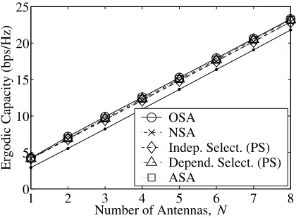
Finally, in Fig. 5 we look at the behavior of joint TX-RX selection at a SNR of 10dB. As shown, the benefit of joint
selection at the TX and RX rather than independent selection at both ends is very slight. Again, the PS approximation is excellent and the improvement over TX selection is only marginal.
The NSA and PMWF by design are low complexity algo-rithms involving the computation of column norms and order-ing only. OSA, on the other hand, is highly intensive requirorder-ing
m
r
×n t
matrix determinants, in addition to ordering and other matrix operations. Hence, the superior performance of of NSA with PMWF at low SNR is quite notable.
VII. CONCLUSION
The NSA is seen to be an important selection method, since its complexity is far less than OSA, its performance is close to OSA and, with the addition of PMWF, it can outperform OSA at low SNR levels. Hence, an analysis method for NSA is important and the power scaling method we have developed is able to approximate capacity for NSA over a variety of channels and system scenarios. The beauty of the PS approach is its generality and its ability to gauge the effect of selection in a single number. In particular, analytical results clearly show the effects of PMWF and imperfect CSI in simple closed-form expressions.
REFERENCES
[1] S. Sanayei and A. Nosratinia, “Antenna selection in MIMO systems,”
IEEE Commun. Mag., vol. 42, no. 10, pp. 68–73, Oct. 2004.
[2] R. S. Blum and J. H. Winters, “On optimum MIMO with antenna selection,”IEEE Commun. Lett., vol. 6, no. 8, pp. 322–324, Aug. 2002. [3] Z. Zhou, Y. Dong, X. Zhang, W. Wang, and Y. Zhang, “A novel antenna selection scheme in MIMO systems,” in Proc. Int’l. Conf. on Communications, Circuits and Systems, Chengdu, China, June 27-29, 2004, pp. 190–194.
[4] R. Heath and A. Paulraj, “Antenna selection for spatial multiplexing systems based on minimum error rate,” in Proc. IEEE Int’l. Conf. on Communications, Helsinki, Finland, 2001, pp. 2276–2280.
[5] Z. Chen, B. Vucetic, and J. Yuan, “Space-time trellis codes with transmit antenna selection,”IEE Electronics Letters, vol. 39, pp. 854–855, May 2003.
[6] A. Molisch, M. Win, and J. Winters, “Capacity of MIMO systems with antenna selection,” inProc. IEEE Int’l. Conf. on Communications, Helsinki, Finland, 2001, pp. 570–574.
[7] M. Gharavi-Alkhansari and A. B. Gershman, “Fast antenna subset selection in MIMO systems,” IEEE Trans. Signal Processing, vol. 52, no. 2, pp. 339–347, Feb. 2004.
[8] A. Molisch and X. Zhang, “FFT-based hybrid antenna selection schemes for spatially correlated MIMO channels,”IEEE Commun. Lett., vol. 8, no. 1, pp. 36–38, Jan. 2004.
[9] I. E. Telatar, “Capacity of multi-antenna Gaussian channels,”European Trans. on Telecomm. Related Technol., vol. 10, pp. 585–595, Nov.-Dec. 1999.
[10] P. J. Smith, S. Roy, and M. Shafi, “Capacity of MIMO systems with semicorrelated flat fading,”IEEE Trans. Inform. Theory, vol. 49, no. 10, pp. 2781–2788, Oct. 2003.
[11] M. Kang and M.-S. Alouini, “On the capacity of MIMO Rician channels,” inProc. 40th Annu. Allerton Conf. Communications, Control, and Computing, Allerton Monticello, IL, USA, Oct. 2002, pp. 936–945. [12] H. David and H. Nagaraja, Eds.,Order Statistics. Hoboken, New Jersey,
USA: John Wiley and Sons Inc., 2003.
[13] N. L. Johnson and S. Kotz, Eds.,Continuous Univariate Distributions-2. Hoboken, New Jersey, USA: John Wiley and Sons Inc., 1970. [14] S. Loyka, “Channel capacity of MIMO architecture using the exponential
1 2 3 4 5 6 7 8 5
10 15 20 25
Number of Antennas, N
Ergodic Capacity (bps/Hz)
[image:6.612.54.498.70.226.2]OSA NSA ASA Rayleigh SC Rayleigh Ricean
Fig. 1. Comparison of selection schemes for a (N,N+ 2) choose (N,N) system (SNR = 10dB).
1 2 3 4 5 6 7 8
5 10 15 20 25
Number of Antennas, N
Ergodic Capacity (bps/Hz)
NSA PA Approx. PS Approx. Rayleigh SC Rayleigh Ricean
Fig. 2. Approximations for NSA for a (N,N+ 2) choose (N,N) system (SNR = 10dB).
1 2 3 4 5 6 7 8
0 2 4 6 8
Number of Antennas, N
Ergodic Capacity (bps/Hz)
OSA NSA
NSA w/ PMWF PS Approx. ASA
Fig. 3. PMWF comparison for a (N,N+ 2) choose (N,N) system for an i.i.d. Rayleigh channel (SNR = 0dB).
0 0.2 0.4 0.6 0.8 1
0.9 1 1.1 1.2 1.3 1.4 1.5
CSI Quality Factor, ρ
Capacity Ratio (C
NSA
/C
ASA
) (2,4) choose (2,2)
(2,4) choose (2,2) (PS) (2,6) choose (2,2) (2,6) choose (2,2) (PS)
Fig. 4. Effect of imperfect channel state information on antenna selection for an i.i.d. Rayleigh channel (SNR = 0dB).
1 2 3 4 5 6 7 8
0 5 10 15 20 25
Number of Antennas, N
Ergodic Capacity (bps/Hz)
OSA NSA
Indep. Select. (PS) Depend. Select. (PS) ASA
[image:6.612.54.499.297.454.2] [image:6.612.55.265.524.679.2]