MATTHEW HENNESSY Department of Computer Science, Trinity College Dublin, Ireland e-mail address: [email protected]
Abstract. We develop a version of the picalculus Picostwhere channels are interpreted asresourceswhich have costs associated with them. Code runs under the financial respon-sibility ofowners; they must pay touse resources, but may profit byproviding them.
We provide a proof methodology for processes described inPicost based on bisimula-tions. The underlying behavioural theory is justified via a contextual characterisation. We also demonstrate its usefulness via examples.
1. Introduction
The purpose of this paper is to develop a behavioural theory of processes, in which computations depend on the ability to fund the resources involved. The theory will be based on the well-known concept of bisimulations, [Mil99], which automatically gives a powerful co-inductive proof methodology for establishing properties of processes; here these properties will include the cost of behaviour.
We take as a starting point the well-known picalculus, [SW01, Mil99], a language for describing mobile processes which has a well-developed behavioural theory. In the picalculus a process is described in terms of its ability to input and output oncommunication channels. Here we interpret these channels as resources, or services, as for example in [CGP08]. So input along a channel, written asc?(x).P in the picalculus, is now interpreted asproviding the servicec, while output, written c!hvi.P, is interpreted as a request to use the servicec. A process is now determined by the manner in which itprovides services anduses them.
Viewed from this perspective, we extend the picalculus in two ways. Firstly we associate a cost with resources; specifically for each resource we assume that a certain amount of funds ku is charged to use it, and an amount kp is also required to provide it. Secondly we introduce principals orowners who provide the funds necessary for the functioning of resources. The novel construct in the language is [P]o, representing the (picalculus) process P running under the financial responsibility of o. For example in [c!hvi.Q]o the use of the resource c is only possible if o can fund the charges. Similarly with [c?(x).Q]o, but
1998 ACM Subject Classification: F.3.1 [Specifying and Verifying and Reasoning about pro-grams]: bisimulations for distributed resources, F.3.2 [ Semantics of Programing Languages ]: op-erational semantics, F.3.3 [Studies of Program Constructs]: resource usage.
Key words and phrases: resources, cost, picalculus, bisimulations, amortisation. The financial support of SFI is gratefully acknowledged.
LOGICAL METHODS
IN COMPUTER SCIENCE DOI:10.2168/LMCS-???
c
Matthew Hennessy Creative Commons
here there is also the potential for gain for owner o; in our formulation o profits from any difference between the cost in providing the resource and the charge made to use it.
Our language Picost is presented in Section 2, and is essentially a variation on Dpi, a typed distributed version of the picalculus, [Hen07]. The reduction semantics is given in terms of judgements of the form
(ΓM)−→(∆N)
where Γ,∆ arecost environments. These have a static component, giving the costs associ-ated with resources, and a dynamic part, which gives the funds available to owners and also records expenditure. The usefulness of the language is demonstrated by a series of simple examples.
But the main achievement of the paper is a behavioural theory, expressed as judgements
(ΓM)⊑
awgt (∆N) (1.1)
indicating that, informally speaking,
(i) the processM running relative to the cost environment Γ is bisimilar, in the standard sense [Mil89], with process N running relative to ∆
(ii) the costs associated with (∆N) are no more, and possibly less, than those associated
with (ΓM).
Influenced by [KAK05] we first develop a general framework of weighted labelled tran-sition systems or wLTSs, in which actions, including internal actions, may have multiple weights associated with them. We then define a notion ofamortised weighted bisimulations between their states, giving rise to a preorder s ⊑awgt t, meaning that s, t are bisimilar but in some sense the behaviours of t are lighter than those of s. From this we obtain, in the standard manner, a co-inductive proof methodology for proving that two systems are related; it is sufficient to find, or construct, a particular amortised weighted bisimulation containing the pair (s, t).
This proof methodology is applied to Picost by first interpreting the language as an LTS, in agreement with the reduction semantics, and then interpreting this LTS as a wLTS, giving rise to (parametrised versions of) the judgements (1.1) above. But as we will see these judgements can be interpreted in two ways. If the recorded expenditure represents costs then (∆N) can be considered an improvement on (ΓM). On the other hand if
it representsprofits then we have the reverse; (ΓM) is an improvement on (∆N) as it
has the potential to be heavier.
The details of this theory are given in Section 3, and the resulting proof methodology is illustrated by examples. However in Section 4 we re-examine this proof methodology, in the light of reasonable properties we would expect of it; and these are found wanting. It turns out that the manner in which we generate the wLTS for Picost from its operational semantics is too coarse. We show how to generate a somewhat more abstract wLTS, and prove that the resulting proof methodology is satisfactory, in a precise technical sense, by adapting the notion of reduction barbed congruence, [HT92, SW01, HR04, Hen07].
2. The language Picost
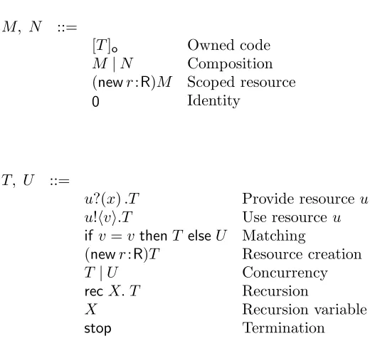
M, N ::=
[T]o Owned code
M|N Composition
(newr:R)M Scoped resource
0 Identity
T, U ::=
u?(x).T Provide resourceu
u!hvi.T Use resourceu
if v=vthenT elseU Matching
(newr:R)T Resource creation
T|U Concurrency
recX. T Recursion
X Recursion variable
[image:3.612.176.436.85.328.2]stop Termination
Figure 1: Syntax ofPicost
identifiers, which may be either resource names or (value) variables. We also assume a set of principals orowners Own containing at least two elements, ranged over by o,u,p, who are implicitly registered for these resources and who finance their provision and use. The syntax of Picost is then given in Figure 1, and is essentially a very minor variation onDpi, [Hen07]. The main syntactic category represents code running under responsibility, with [P]o being the novel construct. As explained in the Introduction this represents the code P running under the responsibility of the owner o; intuitively o is financially responsible for the computation P. Thus in general a system is simply a collection of computation threads each running under the responsibility of an explicit owner, which may share private resources. The syntax for these threads is a version of the well-known picalculus, [SW01].
The type R of a resource describes the costs associated with that resource. There is a cost associated with using a resource, and a cost associated with providing it; therefore types take the form hku, kpi where ku, kp are elements from some cost domain K. Here we take K simply to beN ordered in the standard manner, but most of our results apply
equally well to variations.
We employ the standard abbreviations associated with the picalculus, and associated terminology. In particular we assume Barendregt’s convention, which implies that bound variables used in terms or definitions are distinct, and different from any free variables in use in the current context. In Figure 1 meta-variable vrange overvalue expressions, whose specification we omit; but they include at least resource namesa∈Chan, variables x from
Var, and elements ofK. As usual we omit every occurrence of a trailingstopand abbreviate u?().T, u!hi.T tou?.T, u!.T respectively. We are only interested inclosed code terms, those which contain no free occurrences of variables, which are ranged over by P, Q, . . .; we use
2.2. Cost environments: Since computations have financial implications, the execution of processes is now relative to a cost environment Γ. This records the financial resources available to principals, and the cost of providing and using resources; in order to be able to compare the cost of computations we also assume a component which records the expen-diture as a computation proceeds. Thus judgements of the reduction semantics take the form
ΓM −→ ∆N
where Γ, ∆ are cost environments.
There are many possibilities for cost environments; see [HG08] for an example which directly associates funds with resources. In the present paper we define them in such a way that the owners retain total control over their own funds.
Definition 2.1 (Cost environments). A cost environment Γ consists of a 4-tuple
hΓo,Γu,Γp,Γreciwhere
• Γu:Chan⇀ K
Γu(a) records the cost of using resource a; this is a static component, and will not vary during computations
• Γp:Chan⇀ K
Γp(a) records the cost of providing resource a; again this is a static component
• Γo:Own⇀ K
Γo(o) records the funds available to owner o; this will vary as computations proceed, as owners will need to fund their interactions with resources
• Γrec∈K
Γreckeeps an account of the expenditure occurred during a computation; of course this also will vary as a computation proceeds.
We assume that both functions Γu, Γp have the same finite domain, but not necessarily
that Γu(a)≥Γp(a) whenever these are defined.
We now define some operations on cost environments which will enable us to reflect their impact on the semantics of our language. The most important is a partial function, Γ−−−−→(u,a,p) ∆, which informally means that in Γ owneruhas sufficient funds to cover the cost of using resourceaand ownerphas sufficient funds to provide it. Then ∆ records the result of the expenditure of both o and p of those funds. There is also considerable scope as to what happens to these funds, and how their expenditure is recorded. Here we take the view that the providerp gains the cost which the user expends, to offsetp’s cost in providing the resource.
Definition 2.2 (Resource charging). Let−−−−→(u,a,p) be the partial function over cost environ-ments defined as follows: Γ−−−−→(u,a,p) ∆ if
(i) Γo(u)≥Γu(a) and Γo(p)≥Γp(a)
(ii) ∆ is the cost environment obtained from Γ by (a) decreasing Γo(u) by the amount Γu(a)
(b) increasing Γo(p) by the amount Γu(a)−Γp(a), which may of course be negative (iii) Finally there is considerable flexibility in how this resource expenditure is recorded in
we allow functions reca(−,−), for each resource a, in which case we define ∆rec to be Γrec+rec
a(Γu(a),Γp(a)).
In general we allow the owners u and p in this definition to coincide. So, for example if Γ−−−−→(o,a,o) ∆, then the effect of performing (a) above, followed by (b), is that ∆o(o) is set to Γo(o)−Γp(a).
The use of two independent charges for each resource, Γu and Γp, may seem overly complex. A simpler model can be obtained by having only one combined charge; effec-tively we could assume Γp(a) to be 0 for everya, and so resource charging simply transfers the appropriate amount of funds from the user to the provider; this could be achieved by restricting attention tosimple types, resource types Rof the form hku,0i. Indeed this sim-plification will be quite useful in order to achieve some theoretical properties of our proof methodology; see Definition 4.18 and Section 4.2. Nevertheless the use of the two indepen-dent charges Γp(−) and Γu(−) allows scope for more interesting examples. In particular it provides considerable scope for variation in the manner in which resource expenditure is recorded in the component Γrec; see Example 2.8 for an instance.
We also need to extend cost environments with new resources.
Definition 2.3 (Resource registration). The cost environment Γ, a:R, is only defined if a isfreshto Γ, that is, ifais neither in dom(Γu) nor in dom(Γp). In this case it gives the new cost environment ∆ obtained by adding the new resource, with the capabilities determined by R. Formally the dynamic components of ∆, namely ∆o and ∆rec, are inherited directly from Γ, while the static components have the obvious definition; for example if R is the type hku, kpi then ∆u is given by
∆u(x) = (
ku ifx=a Γu(x) otherwise
We also assume that the resource charging forain (Γ, a:R) is always standard.
Note that every cost environment may be written in the form
Γdyn, a1:R1, . . . an:Rn
where Γdyn is a basic environment; that is the static components Γudyn and Γ p
dyn are both empty, and so it only contains non-trivial dynamic components.
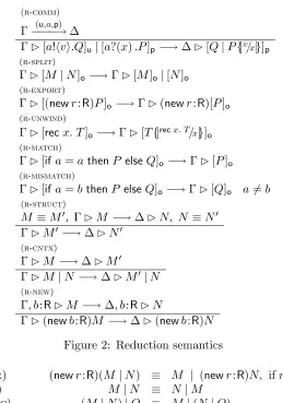
2.3. Reduction semantics: The pair (Γ M) is called a configuration if fn(M) ⊆
dom(Γu) = dom(Γp), that is every free resource name in M is known to the cost envi-ronment Γ. The reduction semantics for Picost is then defined as the least relation over configurations which satisfies the rules in Figure 2. The majority of the rules come directly from the reduction semantics ofDpi, [Hen07], and are housekeeping in nature. The only rule of interest is (r-comm), representing the communication along the channel a, or in Picost
theuse of the resourceaby owneru which isprovided by ownerp. However this reduction is only possible whenever the premise Γ−−−−→(u,a,p) ∆ is satisfied. As we have seen, this means that in Γ owner uhas sufficient funds to cover the cost of using resourceaand ownerphas sufficient funds to provide it; and further ∆ records the result of the expenditure of both u
and p of those funds.
(r-comm)
Γ−−−−→(u,a,p) ∆
Γ[a!hvi.Q]u|[a?(x).P]p−→∆[Q|P{|v/x|}]p
(r-split)
Γ[M|N]o−→Γ[M]o|[N]o
(r-export)
Γ[(newr:R)P]o −→Γ(newr:R)[P]o
(r-unwind)
Γ[recx. T]o −→Γ[T{|recx. T/x|}]o
(r-match)
Γ[ifa=athenP elseQ]o−→Γ[P]o
(r-mismatch)
Γ[ifa=bthenP elseQ]o −→Γ[Q]o a6=b
(r-struct)
M ≡M′, ΓM −→∆N, N ≡N′
ΓM′ −→∆N′
(r-cntx)
ΓM −→∆M′
ΓM|N −→∆M′|N
(r-new)
Γ, b:RM −→∆, b:RN
[image:6.612.173.432.88.457.2]Γ(newb:R)M −→∆(newb:R)N
Figure 2: Reduction semantics
(s-extr) (newr:R)(M |N) ≡ M | (newr:R)N, ifr6∈fn(M)
(s-com) M|N ≡ N|M
(s-assoc) (M|N)|O ≡ M|(N |O)
(s-zero) M |0 ≡ M
[stop]o ≡ 0
(s-flip) (newr:R)(newr′:R′)M ≡ (newr′:R′)(newr:R)M
Figure 3: Structural equivalence of Picost
the standard one from Dpi, the definition of which is given in Figure 3. Also the final rule (r-new) uses the registration operation on cost environments, given in Definition 2.3.
Proposition 2.4. If (Γ1 M1) is a configuration and (Γ1 M1) −→ (Γ2 M2) then
(Γ2M2) is also a configuration.
Proof. Straightforward, by induction on the proof that (Γ1M1) −→ (Γ2M2). When
handling the rule (r-struct) it uses the obvious fact that M ≡ N implies that M and
N have the same set of free names; this in turn means that M ≡ N implies ΓM is a
configuration if and only if ΓN is.
The reductions of a configuration affect its cost environment, and as a sanity check we can describe precisely the kinds of changes which are possible:
Sys⇐( [Reader]pub | [Library|Store]lib) where
Reader⇐recR.goLib?(name).(newr)reqR!hr,namei.
r?(b).goHome!hbi.R
Library⇐recL.reqR?(y, z). y!hbook(z)i.L
⊕(newr)reqS!hr, zi.r?(b).y!hbi.L
Store⇐recS.reqS?(y, z).y!hbook(z)i.S
Figure 4: Running a library
(i) Γ1= Γ2, and (∆M1)−→(∆M2) whenever (∆M1) is a configuration
(ii) or Γ1 (u,a,p)
−−−−→Γ2, for some resource a and owners u, p, and whenever (∆M1) is a
configuration ∆−−−−→(u,a,p) ∆′ implies (∆M1)−→(∆′M2)
(iii) orΓ1, a:R (u,a,p)
−−−−→Γ2, a:R, for some (fresh) resourcea, resource typeRand ownersu, p,
and whenever(∆M1)is a configuration ∆, a:R−−−−→(u,a,p) ∆′, a:Rimplies(∆M1)−→
(∆′M
2)
Proof. Again this is a simple proof by rule induction on the premise (Γ1M1)−→(Γ2M2).
Intuitively possibility (i) corresponds to a move where no communication occurs, (ii) is when the move is a communication along a channel a known to Γ1, and (iii) when the
communication is along a private internal channel.
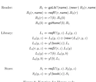
2.4. Examples: FormallyPicosthas only unary communication, but in these examples we will informally allow the communication of tuples along channels. In addition we will use the standard abbreviations associated with the picalculus. We also omit types for channels when they are not relevant; in such cases we assume that they cost nothing to provide, and that there is no charge for using them. It will be convenient to have an internal choice operator, with P⊕Qrepresenting an internal choice between P and Q. This can be taken to be short-hand notation for (newc)(c!hi |c?().P |c?().Q), where c is a fresh channel.
Example 2.6 (Running a library). Consider the system Sysfrom Figure 4, which consists of three recursive components, a library user Reader, running under the responsibility of the principal pub, standing for public, a library interface Library and an auxiliary book depositoryStore, both running under some other principallib.
The programming of these components involves the systematic generation ofreply chan-nels. Thus for example theReadergets the name of a book with which to go to the library, generates a new reply channelr and submits this together with the name of the book via
Let us now consider the behaviour of these systems relative to two cost environments Γlocal, Γcentral representing two different strategies for providing library services. To focus on the relative cost of providing these services let us assume that their use is free, that is Γu
∗(a) = 0 for every resource a, where∗ ranges over local,central, and that the amount of funds available is not an issue, that is Γo
∗(pub) = Γo∗(lib) = ∞. The cost of providing the services, Γp∗ is given in the table below, reflecting on the one hand the relative convenience to theReaderof the local services, and on the other the relative convenience to the authorities in providing central services.
local central
goLib 1 5
goHome 1 5
reqR 3 1
reqS 5 1
Finally let us take the counters Γrec∗ to be initially set to 0. Note that Γlocal can be written as
Γdyn, goLib:Rgl, goHome:Rlh, reqR:Rrl, reqS:Rsl
where Rgl,Rhl,Rrl,Rsl are the types h0,1i,h0,1i,h0,3i,h0,5i respectively, and Γdyn is a basic environment; Γcentralhas a similar representation, with a slightly different sequence of types.
To exercise the system we use
Book⇐[goLib!hstri.goHome?(x).stop]pub
to prod the Reader into action, wherestris the name of some book. Consider the configu-ration
C1 = Γlocal(Book|Sys),
and let us ignore the computation steps involved in generating reply channels, and general housekeeping such as the unwinding of recursive definitions, which in any event cost nothing. Because of the internal non-determinism in the library service there are essentially two computations from C1. If the Store is not used then after three computation steps which
require funds it is in the state ∆localSys, where ∆reclocal = 5. This represents the overall cost of this transaction, 2 of which is paid bypub and 3 bylib.
On the other hand if theStoreis used, then there are four computation steps which re-quire funding, after which the state ΘlocalSysis reached, where Θrec
local = 10. However using
the central cost environment Γcentral the two possibilities are ∆rec
central= 11 and Θreccentral= 12 respectively. In each eventuality the local implementation is more efficient, in the sense
that the costs are systematically lower.
Sys⇐[P]p | [N]n | [A]a | [R]r where
P ⇐recP.(newr1)news!hr1i.(newr2)adv!hr2i.
r1?(n).r2?(d).publish?(z).z!hn, di.P
N ⇐recN.news?(r) (newn)r!hni.N A⇐recA.adv?(r).(newd)r!hdi.A R⇐recR.(newr)publish!hri.r?(n, d).R
Figure 5: Publishing
Example 2.7 (Fund transfer). Consider the systems defined as follows:
Sys⇐[D]dad |[K]kate where
D⇐req?(x).(news:Rs)x!hsi.s!.S K ⇐(newr)req!hri.r?(y).y?.H
The size of the transfer from dadto katedepends on the type Rs at which the new channel sis declared. Suppose this type ish0, ki, and let Γ be a cost environment in which Γo(dad) is at least k. Then there is a computation
(ΓSys) −→∗ (∆[S]dad |[H]kate)
in which ∆o(dad) = Γo(dad)−k and ∆o(kate) = Γo(kate) +k.
Example 2.8 (Publishing). Consider the system Sys in Figure 5, which has four compo-nents:
(a) publisher: uses a news service via the resourcenews,uses an advertising agency via the resource adv and provides the resource publish
(b) news service: provides a service via news
(c) ad agency: provides a service via adv
(d) reader: uses the resourcepublish
The viability of publishing depends of course on the cost associated with these resources. As an example consider an environment Γ327, of the form Γdyn,news:Rn,adv:Ra,publish:Rp, where these types are h3,1i,h2,0i,h7,1i respectively, and let us assume Γrec327 is initialised to 0. Furthermore, since we are concentrating on the publisher, let us assume that the resource charging is defined so that only the effect on the owner p is recorded. Refering to Definition 2.2 this means that resource charging is standard forpublish but we need to set reca(ku, kp) to be−ku, ifa is either newsoradv.
Now consider a computation from the configuration Γ317Sys. Provided the owners
have sufficient funds, specifically Γo(p),Γo(n) and Γo(r) must be at least 5,1,7 respectively, then we have a computation
(Γ317Sys)−→∗ (∆1Sys)
where ∆rec
1 = 1; the record part of the initial environment was set to 0, during the
adv; finally, when the reader uses thepublishresource, this is increased by (7−1) to give 1. Because we have defined expenditure recording to reflect the point of view of the publisher, this represents the fact that the publisher has made a profit of 1 as a result of this sequence of transactions. Note also that at this point ∆o
1(p) is Γo327(p) + 1.
We can also see what happens when the costs of using resources is changed. Let Γ216
be the environment in which the cost of all three resources are decreased by 1. Then we have the computation
(Γ216Sys)−→∗ (∆2Sys)
where now ∆rec2 = 2; this represents an increase in profits for the publisher.
Example 2.9 (Kickbacks). Suppose in Figure 5 we change the situation so that the pub-lisher obtains a kickback from the ad agency when an ad is downloaded. The modified code is given by
PK ⇐recP.(newr1)news!hr1i.(newr2)(newk:K)adv!hk, r2i.
r1?(n).r2?(d).publish?(z).k?.z!hn, di.P
AK ⇐recA.adv?(k, r).(newd)r!hdi.(A|k!)
and letSysK denote the revised system. The size of the kickback depends on the parameters in the type K. In Sys the ad agency receives the benefit 2 for supplying the ad; if we set
K to beh1,0i then inSysK this benefit is split equally with the publisher. Under the same assumptions as in Example 2.8 we have the computations
(Γ327SysK)−→∗(Φ1SysK) and (Γ216SysK)−→∗(Φ2SysK) where now Φrec
1 ,Φrec2 are 2,3 respectively, indicating more profit in each case for the
pub-lisher.
3. Compositional reasoning
The aim of this section is to develop a proof methodology for Picost. The idea is to define abehavioural preorder
(ΓM)⊑(∆N), (3.1)
meaning that in some sense (ΓM) and (∆N) offer the same behaviour, but the latter
is at least as efficient as the former, and possibly more. We follow the standard approach of defining the preorder (3.1) as the largest relation betweenPicostconfigurations satisfying a transfer property, associated with the ability of processes to interact with their peers. We thereby automatically get a co-inductive proof methodology for establishing relationships between configurations.
In fact, referring to (3.1), it is better to move away from terminology such asefficiency as the interpretation depends very much on the nature of the units being recorded. In Example 2.6 these are costs and in such a scenario it is reasonable to interpret (3.1) as saying (∆N) is an improvement on (ΓM) as it potentially involves less cost. On the
other hand in Example 2.8 the units are profit (for the publisher), and here (ΓM) would
be considered to be an improvement on (∆N), as there is potential for more profit (for
We therefore move to the more neutral terminology of weights. However we can not simply base the formulation of (3.1) on the relative weight associated with each individual action, as the following example shows.
Example 3.1 (Amortising costs). Consider the simple system
UD⇐[recx.up!.down!.x]o
and let Γ25 be an environment in which the unique ownerohas unlimited funds, the use of upcosts 2 and the use ofdowncosts 5. If we compare (Γ25UD) with (Γ42UD), where Γ42
is defined analogously, then intuitively the latter is more efficient than the former, despite the fact that in the latter the action up is more expensive; this is compensated for by the
relative costs of the other action down.
The remainder of this section is divided into three subsections. In the first we present a theory of amortised weighted bisimulations, based on so-called weighted labelled transition systems, wLTSs. This gives rise to a parametrised behavioural preorder, which we call the amortised weighted bisimulation preorder. The aim is to apply this theory to Picost; with this in mind, in the second subsection we present a (detailed) labelled transition semantics forPicost, and show that it is in agreement with the reduction semantics given in Figure 2. In the third section we show how this automatically generates a wLTS, which in turn gives us an amortised weighted bisimulation preorder between Picost configurations. We demonstrate the usefulness of the resulting proof methodology by re-examining the examples from Section 2.4.
3.1. Amortised weighted bisimulations: Here we generalise the concepts of [KAK05]; our aim is to apply them toPicost but our formulation is at a more abstract level.
Definition 3.2 (Weighted labelled transition systems). An weighted labelled transition system or wLTS is a 4-tuplehS,Actτ, W,−−→i whereS is a set of states, W set of weights, and −−→ ⊆ S×Actτ ×W ×S. Here Actτ denotes a set of action names Act to which is added an extra distinct name τ which will represent internal action. We normally write s−−→µ ws′ to mean (s, µ, w, s′) ∈ −−→. As a default we take the set of weights to be Z, the
set of integers, both negative and positive.
A wLTS is called standard whenever there is a cost function weight : Act → W with the property that s−−→a ws′ if and only ifw=weight(a) for everya∈Act. So in a standard wLTS there is a unique weight associated with external actions, although internal actions may have multiple possible associated weights, reflecting the different ways in which these actions may be generated from external moves. The wLTS which we will (eventually) generate for Picost will be standard, but the development below will not require that we are working with standard wLTSs.
Relative to a given wLTSweak moves are generated in the standard manner, although the associated weights need to be accumulated: s==µ⇒ws′ is the least relation satisfying:
• s−−→µ ws′ implies s µ = =⇒w s′
• s==µ⇒w s′′, s′′−−→τ vs′ impliess µ =
=⇒(w+v)s′ • s−−→τ ws′′, s′′
µ =
=⇒v s′ impliess µ =
We also use a variation on the standard notation s ==µˆ⇒w t from [Mil89]; when µ is any action other thanτ this denotes s==µ⇒wt, but when it is τ it means either thats
τ =
=⇒wtor thats istand w= 0.
Definition 3.3 (Amortised weighted bisimulations). A family of relations { Rn | n∈N} over the states in a wLTS is called anamortised weighted bisimulation wheneversRnt:
(i) s−−→µ vs′ impliest
ˆ
µ =
=⇒w t′ for somet′, w such thats′R(n+v−w)t′ (ii) conversely,t−−→µ wt′ impliess
ˆ
µ =
=⇒v s′ for somes′, v such that s′R(n+v−w)t′
Here the parametrisation with respect to N puts an extra requirement on the standard
transfer properties associated with bisimulations. In (i) and (ii) above the index (n+v−w) must be in N, that is must be non-negative. So for example if the amortisationnis 0 then
v, the weight of the left hand action, must be greater than or equal to w, the weight of the right hand action. For this reason a standard bisimulation, which ignores the weights, may not be an amortised weighted bisimulation. But the more general effect of the parametern in the definition is to allow a relaxation in the comparison between the actual weights of the actions in the processes being compared; this point is explained in detail in Example 3.6.
We can mimic the standard development of bisimulations and write s ⊑m
wgt s′ to say
that there is some amortised bisimulation { Rn | n ∈ N} such that sRm s′. Weighted bisimulations are (point-wise) closed under unions, and therefore we can mimic the standard development of bisimulation equivalence, [Mil89], to obtain the following:
Proposition 3.4.
(a) The family of relations { ⊑n
wgt| n∈N} is an amortised weighted bisimulation.
(b) This family is the largest (point-wise) amortised weighed bisimulation. (c) If s⊑m
wgtt and s
µ =
=⇒v s′ then t
ˆ
µ =
=⇒w t′ for some t′, v such that s′ ⊑(wgtm+v−w) t′.
Proof. Straightforward, using standard techniques.
When we are uninterested in the exact amortisation used we write simply s ⊑wgt t, meaning that there is some k≥0 such that s⊑k
wgt t, and we refer to this preorder as the
amortised weighted bisimulation preorder.
Proposition 3.5.
(a) The relations ⊑n
wgt are reflexive
(b) s1 ⊑mwgt s2, s2 ⊑nwgt s3 implies s1 ⊑(wgtm+n)s3
(c) ⊑m
wgt ⊆ ⊑nwgt whenever m≤n.
Proof. In each case it is sufficient to exhibit a suitable amortised weighted bisimulation, that is a suitable family of relations over states. For example to prove (b) we let Rk, for k≥0, be the set of pairshs1, s2isuch that s1⊑nwgt s3 and s3 ⊑mwgts2 for some state s3 and
some numbersn, m such thatk=n+m.
To show { Rk | k∈N}is an amortised weighted bisimulation let us supposes
1Rks2
and s1
µ
−
−→vs′1; we have to prove
s2 ˆ
µ =
=⇒ws′2 for somes′2 satisfyings′1R(k+v−w)s′2 (3.2)
(The proof of the symmetric requirement is similar.)
(i) From s1⊑nwgt s3 we know s3 ˆ
µ =
=⇒u s′3 such that s′1 ⊑(
(ii) Froms3 ⊑mwgt s2, and the final part of the previous Proposition, we know s2 ˆ
µ = =⇒w s′2
such thats′3 ⊑(wgtm+u−w)s′2.
But since (n+v−u)+ (m+u−w) = (k+v−w) we haves′1R(k+v−w)s′
2 and the requirement
(3.2) follows.
The proof of part (c) is similar using the family of relations { Rn | n ∈ N}, where sRntwhenever s⊑m
wgtt for somem≤n, while the proof of part (a) uses the family where
each Rn is the identity relation.
Example 3.6 (Amortising costs continued). Here we continue with Example 3.1. Shortly we will see a systematic way of associating weights with actions in Picost. But informally we can simply say
C25
up!
−−→2 D25 −−−→down! 5 C25
where C25, D25 are abbreviations for the configurations (Γ25 UD) and (Γ25
[down!.rec x. up!.down!.x]o) respectively, and analogously for (Γ42 UD). Then relative
to this induced wLTS we can show that the following is a weighted bisimulation:
Rn={hD
25,D42i} ∪ { hC25,C42i | n≥2}
It follows that
(Γ25UD)⊑2wgt (Γ42UD)
However (Γ42UD) 6 ⊑kwgt(Γ25UD) for anyk. To see this suppose{ Rn | n≥0} is
a weighted bisimulation; we prove by induction onk that
hD42,D25i 6∈ R(k+2) (3.3)
hC42,C25i 6∈ Rk
First notice that the pairhD42,D25ican not be inR2; this is because the moveD42
down! −−−→2C42
can not be matched by a move D42 ===down⇒! w C42 such that C42R(2+2−w)C25.The only only possible candidate is the move D42===down⇒5! C42 and R−1 does not exist.
From this fact it follows immediately that the pair hC42,C25i can not be in R0; for
matching the move C42−−→4up! D42 would require the impossible, that hD42,D25i be R2. In other words we have shown (3.3) in the case whenk= 0.
Suppose it is true for k; the proof that it follows for (k+ 1) is also straightforward. This is because
• for hD42,D25i to be in R(k+3) we would require that hC42,C25i be in R(k+3+2−5)
which contradicts the induction hypothesis
• forhC42,C25ito be in R(k+1) we would requirehD42,D25i to be inR(k+3), which we
have just shown not to be possible.
It is important that the set of natural numbersNis used in Definition 3.3, or at least that
the family of relations be parametrised relative to a well-founded order. If instead we allowed families of relations{Rz | z∈Z}, whereZis the set of all integers, positive and negative, then (Γ42UD)⊑0wgt (Γ25UD) would follow. Simply lettingRz ={hC42,C25i,hD42,D25i}
for every z ∈ Z, we would obtain an extended family of relations trivially satisfying the
difference between amortised weighted bisimulations and standard bisimulations (where all
weights are ignored).
3.2. An operational semantics for Picost. As a first step in applying the theory of amortised weighted bisimulationstoPicostwe give an operational semantics for the language in terms of a (standard) LTS.
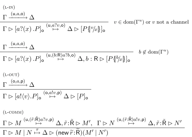
In Figure 6 and Figure 7 we give a set of rules for deriving judgements of the form
(ΓM)7→λ (∆N),
whereλcan take one of the forms (i) internal action, τ
(ii) input, (u,(˜r: ˜R)a?v,p): input by resourceaof a known or fresh name, or value, where
p is the provider of the resource andu the user
(iii) output: (u,(˜r: ˜R)a!v,p): delivery of a known or fresh name, to resourcea, where again
p is the provider of the resource andu the user.
We restrict attention to well-formed λ, that is, in the input and output actions each ri must occur somewhere in v, and applications of the rules must preserve well-formedness. However note that because Picost only uses unary communication the vectors ˜(r),(b) will˜ have length either 0 or 1.
The rules are inherited directly from the corresponding ones for Dpi, [Hen07], and for the sake of clarity obvious symmetric rules, such as for (l-comm) and (l-cntx), are omitted;
Barendregt’s convention is also liberally applied, for example in omitting side-conditions to (l-cntx). The only point of interest is the use of the preconditions Γ−−−−−→(o1,a,o2) ∆ in (l-in)
and (l-out); communication is only deemed to be possible if it can be paid for in some
manner. Note that u in (l-in), and p in (l-out) are free meta-variables. So for example
the simple process [a!hvi.P]o can perform the actions [a!hvi.P]o (o,a!v,o
′)
7→ ∆[P]o for every
owner o′∈Ownsuch that Γ−−−−→(o,a,o′) ∆. Also in the communication rule (l-comm) any new
resources used in the communication, ˜r: ˜Rremain private but in general the resulting cost environment ∆ will be different from Γ; the internal communication involves the use of a resource, and the change from Γ to ∆ will reflect the associated costs.
We can perform a number of sanity checks on these rules. For example one can show that if (Γ1 P1) (b:7→R)α (Γ2 P2) then Γ2 = ∆, b:R for some ∆ such that Γ1−−−−→(u,a,p) ∆,
for some u,p, where a is the channel used in α; a more detailed analysis of the possible judgements is given in the two lemmas below. The actions also preserve configurations:
Proposition 3.7. If(Γ1M1)is a configuration and(Γ1M1)7→λ (Γ2M2)then(Γ2M2)
is also a configuration.
Proof. A straightforward induction on the inference of the judgements.
We also have a consistency check with respect to the reduction semantics of Section 2, stated in the theorem below; the proof requires two technical lemmas.
Lemma 3.8 (Deriv-output). Suppose ΓM (u,(˜r:˜7→R)a!v,p)∆N. Then
(l-in)
Γ−−−−→(u,a,o) ∆
Γ[a?(x).P]o (u,a7→?v,o)∆[P{|v/x|}]o
v∈dom(Γu
) orvnot a channel
Γ−−−−→(u,a,o) ∆
Γ[a?(x).P]o (u,(b:7→R)a?b,o)∆, b:R[P{|b/x|}]o
b6∈dom(Γu )
(l-out)
Γ−−−−→(o,a,p) ∆
Γ[a!hvi.P]o (o,a7→!v,p)∆[P]o
(l-comm)
ΓM (u,(˜r:˜7→R)a?v,p)∆,r˜: ˜RM′, ΓN (u,(˜r:˜7→R)a!v,p)∆,r˜: ˜RN′
ΓM|N 7→τ ∆(newre:Re)(M′|N′)
Figure 6: An action semantics forPicost: main rules
(l-open)
Γ, b:RM (u,a7→!b,p)Γ′M′
Γ(newb:R)M (u,(b:7→R)a!b,p)Γ′M′
a6=b (
l-export)
Γ[(newr:R)P]o 7→τ Γ(newr:R)[P]o
(l-split)
Γ[M|N]o7→τ Γ[M]o|[N]o
(l-unwind)
Γ[recx. T]o 7→τ Γ[T{|recx. T/x|}]o
(l-match)
Γ[if a=athenP elseQ]o 7→τ Γ[P]o
(l-mismatch)
Γ[ifa=bthenP elseQ]o 7→τ Γ[Q]o
a6=b
(l-cntx)
ΓM 7→λ Γ′M′
ΓM|N 7→λ Γ′M′|N
(l-cntx)
Γ, b:RM 7→λ Γ′, b:RM′
Γ(newb:R)M 7→λ Γ′(newb:R)M′
[image:15.612.145.469.87.319.2]b6∈n(λ)
Figure 7: An action semantics forPicost: more rules
(ii) Γ−−−−→(u,a,p) Γ′
(iii) M ≡(newr˜: ˜R)(M′|[a!hvi.Q] u) (iv) N ≡(M′|[Q]u)
(v) ΘM (u,(˜r:˜R)α,p ′)
7→ Θ′,r˜: ˜RN whenever Θ (u,a,p ′)
Proof. By induction on the derivation of ΓM (u,(˜r:˜7→R)a!v,p)∆N.
Lemma 3.9 (Deriv-input). Suppose ΓM (u,(˜r:˜R7→)a?v,p)∆N. Then
(i) ∆ = (Γ′,r˜: ˜R) for some Γ′
(ii) Γ−−−−→(u,a,p) Γ′
(iii) M ≡(new˜c:C)([a?(x).T]p|M′) (iv) N ≡(newc˜:C)([T{|v/x|}]
p|M′)
(v) ΘM (u
′,(˜r: ˜R′)α,p)
7→ Θ′,r˜: ˜R′ N whenever Θ (u ′,a,p)
−−−−→Θ′, for any owner u′, and types ( ˜R′).
Proof. Again a straightforward induction on the derivation ΓM (u,(˜r:˜R7→)a?v,p)∆N. Note
that in part (v) arbitrary types ( ˜R′) can be used because there is no restriction on the type
Rin the second part of the rule (l-in) in Figure 6.
Theorem 3.10. ΓM −→∆N if and only ifΓM 7→τ ∆N′ for some N′ such that
N ≡N′.
(Outline). First we need to show the auxiliary result that structural equivalence is preserved by actions. That is ΓM 7→λ ∆M′ and M ≡ N implies ΓN 7→λ ∆N′ for some
N′ such that M′ ≡ N′; this is proved by induction on the proof of the fact that M ≡N from the rules in Figure 3. Then a straightforward proof by induction on the derivation of ΓM −→∆N from the rules in Figure 2 will show that this implies ΓM 7→τ ∆N′
withN ≡N′; the auxiliary result is required when considering the rule (r-struct). To prove the converse we also employ the two previous lemmas, giving the structure of input and output actions. Suppose ΓM 7→τ ∆N; we prove by rule induction that
ΓM −→ ∆N. The only non-trivial case is when this judgement is inferred using the
rule (l-comm), or its dual. So without loss of generality we know • M =M1|M2
• N = (newr˜: ˜R)(N1|N2)
• ΓM1(u,(˜r:˜R7→)a?v,p)∆,r˜: ˜RN1
• ΓM2(u,(˜r:˜7→R)a!v,p)∆,r˜: ˜RN2
The previous two lemmas can now be applied to obtain the structure ofM1, M2, N1 andN2,
up to structural equivalence; by rearrangingM1|M2, again using the structural equivalence
rules, an application of (r-comm) followed by one of (r-struct) gives the required Γ
M −→∆N.
3.3. A proof methodology for Picost. The operational semantics given in the previous subsection can be used in a straightforward way to obtain a wLTS forPicostconfigurations. It suffices to attach a weight to the actions, which can be done in a systematic manner: we write
(ΓM)−−→µ w(∆N)
whenever
• w= (∆rec−Γrec)
Note that the weight associated with an action is ultimately determined by the manner in which expenditure is recorded in the cost environments; this may reflect the cost of providing the resource in question, as in Example 2.6, the profit to be gained by a particular owner in the use of the resource, as in Example 2.8, or combinations of such concerns.
We can now apply Definition 3.3 to this wLTS to obtain a family of preorders (ΓM)⊑n
wgt (∆N) (3.4)
between Picost configurations. However we must be somewhat careful here, as some of the actions used involve bound names; but by a systematic application of Barendregt’s convention, mentioned on page 3, confusions between these and free names can be avoided. As is well-known, the relations (3.4) come equipped with a powerful co-inductive proof methodology. In order to prove (ΓM) ⊑k
wgt (∆N) for a particular k it is sufficient
to exhibit a family of relations { Rn | n ∈ N} which satisfy the transfer properties of Definition 3.3, such that Rk contains the pair (ΓM,∆N). In the remainder of this section we apply this proof methodology to the examples in Section 2. This allows us to now reason about the behaviour of systems, how they interact with other systems, rather than reason simply about their computation runs.
Example 3.11 (Running a library, revisited). Refering to the definitions in Example 2.6, by exhibiting a witness weighted bisimulation it is possible to show
(Γcentral[Reader]pub)⊑0
wgt (Γlocal[Reader]pub)
This is despite the fact that the local use of the service reqR is more expensive than the central use; this is compensated for by the fact that both goLib and goHome are less ex-pensive locally. It is also worth noting that although the use of resources in both Γcentral and Γlocal is free, in the generated wLTS the output actions actually have non-zero weights associated with them. For example, a typical run in this wLTS from (Γcentral[Reader]pub)
takes the form
(Γcentral[Reader]pub) −−−−−→goLib?n 5. . .−−−−−−−−→(r)reqR!(r,n) 1. . .−−−−−−→goHome!b 5. . .
whereas the corresponding local run is
(Γlocal[Reader]pub)
goLib?n
−−−−−→1. . .
(r)reqR!(r,n) −−−−−−−−→3. . .
goHome!b
−−−−−−→1. . .
To compare the efficiency of the library service itself we consider the following definitions
Liblocal ⇐(new reqS:Rls)([Library|Store]lib)
Libcentral⇐(new reqS:Rcs)([Library|Store]lib)
where, as explained in Example 2.6,Rsl, Rsc, are the typesh0,5i,h0,1irespectively; here the interaction between the library and the store has been internalised, with types reflecting the relative cost of local and central access. Both these configurations simply provide the servicereqR, and viewed in isolation the local service is not more efficient than the central one; no matter what nwe choose, we have
(ΓcentralLibcentral)6 ⊑nwgt(ΓlocalLiblocal) (3.5)
However if we combine the library service with the reader then the overall systems is locally more efficient than the centralised one:
(ΓcentralSys
where
Syslocal ⇐(new reqR:Rlr)([Reader]pub | Liblocal)
Syscentral⇐(new reqR:Rcr)([Reader]pub | Libcentral)
We should point out that in (3.5) and (3.6) we have used the full cost environments
Γlocal, Γcentral, despite the fact that some of the resources have been restricted in the systems;
this is simply in order to avoid the definition of even more environments.
As an example of how such statements can be proved see the Section A.1 in the appendix
for a witness bisimulation which establishes (3.6).
4. Contextual characterisation
In the previous section we have demonstrated that the preorders⊑n
wgt provide a useful
co-inductive methodology for comparing the behaviour of processes, relative to resource costs. In this section we critically review its formulation, revealing some significant inade-quacies, and offer a revised version where these are addressed.
Informally we would expect at least the following two properties of a proof methodology: (a) It should support compositional reasoning, whereby the analysis of process behaviour
can be carried out structurally.
(b) Soundness: Any relationship established between the behaviour of processes using the proof methodology should be justifiable in some independent manner.
Further we could hope for:
(c) Completeness: any pair of processes which are intuitively behaviourally related, should be provably related using our methodology.
Relative to our language Picostthe first criteria, (a), is straightforward to formalise, as a property of the preorders⊑n
wgt.
Definition 4.1 (Compositional). A relation R over Picost configurations is said to be compositional whenever (ΓM) R (∆N) implies
(i) (ΓM|O) Rm (∆N|O), provided (ΓM|O) and (∆N|O) are configurations
(ii) (Γ, r:RM) Rm (∆, r:RN).
We could of course demand that the relationRshould be preserved by all the operators in the language, but for the purposes of the discussion to follow it is sufficient to concentrate on the two most important ones.
Our first remark is that the relations ⊑n
wgt are not compositional, and therefore our
proposed proof methodology does not support compositional reasoning.
Example 4.2 (Non-compositionality). Let Γ be a cost environment with two owners o,p
and two resourcesa, b. Suppose further that Γo(o) = Γo(p) =∞, while Γu(a) = 20, Γu(b) = 10; the remaining fields in Γ are unimportant, but to be definite let us say that Γp(a) = Γp(b) = 0. Let ∆ be another cost environment with the same resources, with both usage costs being 10, and the same owners, but with the difference that ∆o(o) = 10. Then it is easy to check that
Γ[a!]o⊑0
However one can also show that
Γ[a!]o|[b!]o6 ⊑0
wgt∆[a!]o|[b!]o
The problem occurs when we consider the action (Γ[a!]o|[b!]o)(o7→,b!,p)10(Γ1[a!]o|[stop]o).
This can be matched by the action (∆[a!]o |[b!]o) (o7→,b!,p)10 (∆1 [a!]o|[stop]o) but at
the expense of exhausting all of o’s funds. ∆o
1(o) is now set to 0 and therefore the action
(Γ1[a!]o |[stop]o) (o,a!,p)
7→ 20 (Γ1[stop]o|[stop]o) can not be matched by any action from
(∆1[a!]o|[stop]o).
The other criteria, (b) and (c) above, are more difficult to formalise. But even in the absence of a precise formalisation we can also show that our proof methodology runs into difficulties with them, by considering a proposed touchstone family of preorders ⊑n
behav
, n≥0, which incorporate some intuitive properties which we would expect. First an easy example, essentially taken from [HR04].
Example 4.3 (Problem with output types). Consider the two configurations C and D, denoted by
Γ(newr:R1)([a!hri.stop]o), Γ(newr:R2)([a!hri.stop]o)
respectively, where the typesR1, R2 are different, and Γ has sufficient resources for ato be
exercised; that is Γ−−−−→(o,a,p) Γ′ for some owner p and some Γ′. Then it is easy to see thatC 6 ⊑k
wgtDfor any k because the only actions which the
con-figurations can perform are different; they are labelled (p,(r:R1)a!r,o) and (p,(r:R2)a!r,o) respectively.
However it is difficult to envisage any context in which these two configurations can be distinguished; for any reasonable definition of the touchstone relations we would expect
C ⊑k
behavD to be true. Thus our proof methodology will not becomplete.
Our next example focuses on some of the novel features ofPicost.
Example 4.4 (Problem with owner identification). Let C, D denote the configurations Γ[a!]o
1, Γ[a!]o2
respectively, where o1, o2 are two different owners, and Γo(o1) = Γo(o2).
Here again we would expect C ⊑k
behav D to be true because there is no mechanism in Picostwhich would enable an observer to discover who was funding the use of the resource a. However assuming some owner p has sufficient funds in Γ to provide the resource a, we haveC 6 ⊑0
wgtDagain because the configurations perform different actions, labelled (o1, a!,p)
and (o2, a!,p) respectively.
4.1. Behavioural preorders. In order to address the inadequacies with our proof method-ology let us first give one possible formalisation of the touchstone family of behavioural preorders which we have been refering to as⊑n
behav, n≥0; we adapt the theory ofreduction
barbed congruences, [HT92, SW01, HR04] toPicost, often refered to informally ascontextual equivalences. For simplicity we assume that resource charging is always standard, and that the only values used are channel/resource names.
the reduction rules, in Figure 2, and (∆rec−Γrec) =c. This is generalised in the obvious manner to ΓM −→∗
d∆N by the accumulation of costs.
Definition 4.5 (Cost improving). We say that the family of relations { Rn | n∈N}over configurations iscost improving whenever C Rm D for any m, then
(i) C −→c C′ implies D −→∗dD′ such that C′R(m+c−d)D′
(ii) conversely,D −→dD′ impliesC −→∗c C′ such thatC′R(m+c−d)D′.
This is a natural generalisation of the notion ofreduction closure orreduction bisimulation from LTSs to weighted LTSs; for a justification of its use in defining behavioural preorders see Chapter 2 of [SW01].
Definition 4.6(Observations). Let us write (ΓM)⇓a? whenever (ΓM)−→∗(∆N)
where for some ownero
(i) N ≡(newc)([a?(x)˜ .T]o|N′), andadoes not occur in (˜c)
(ii) ∆−−−−→(u,a,o) ∆′ for someu and ∆′.
The predicate (ΓM)⇓a! is defined in an analogous manner. Note that here the ownero
has to be able to pay the appropriate costs for the barb.
Then we say that the family of relations { Rn | n ∈N} over configurationspreserves observations whenever, for any n,C1RnC2 C1⇓oif and only if C2⇓o.
Note that unlike [HG08] we do not record the cost of making observations; nor do we observe the owner responsible for the observation. This means that our notion of barb is more elementary.
Example 4.2 demonstrates that demanding a behavioural preorder to be compositional, in particular that it be preserved by arbitrary parallel contexts, is very problematic as intuitively it gives observers or external users of a system access to all the funds available to owners of the system. Here we address this issue by defining a relativised version of compositionality, relativised to the set of owners whose funds are available to external users.
Definition 4.7 (O-contextual). Let O be a subset of the owners Own. A relation Rover
Picost configurations is said to beO-contextual whenever (ΓM) R (∆N) implies
(i) (ΓM |[P]o) R (∆N |[P]o) for every o ∈ O , provided (ΓM |[P]o) and
(∆N|[P]o) are configurations.
(ii) (Γ, r:RM) R (∆, r:RN).
Combining these three properties we obtain:
Definition 4.8 (The contextual improvement preorder). Let { ⊑n
O:cxt| n ∈ N} be the
largest family (point-wise) of O-contextual relations over configurations which preserves
observations, and is cost improving.
We now set ourselves the task of modifying the proof methodology of Section 3.3 so that the informal properties (a), (b), and (c) are enforced, relative to the touchstone preorders
⊑n
O:cxt. First note that Example 4.4 and Example 4.3 still apply when the informal relations ⊑n
behav are instantiated by the formal⊑nO:cxt. But the problems presented in Example 4.2
depend on the choice of observersO:
Example 4.9 (Unsoundness). Let Γ, ∆ be as defined in Example 4.2. Then we have already argued that Γ[a!]o ⊑0
wgt ∆[a!]o.Here we argue that Γ[a!]o 6 ⊑0O:cxt∆[a!]o.
whenever o∈O. For otherwise, this would imply Γ[a!]o|[P]o⊑0O
:cxt∆[a!]o|[P]o
for any processP which ensures that the configurations are still well-formed.
However for a contradiction take P to bea?.(b!|b?.ω!) where ω is some cost-free fresh channel. Then we can make the observation ω! on the left hand configuration but not on
the right hand one.
This example shows that in generalO-observers can deplete the resources of any owner inO, which is important if those owners have only finite funds. A significant consequence is given in the next proposition, which limits the applicability of this behavioural preorder for arbitrary O.
Proposition 4.10. If (ΓM)⊑n
O:cxt (∆N) for any n, then Γo(o) = ∆o(o) for every o
in O.
Proof. Suppose (ΓM)⊑n
O:cxt(∆N) for some n, witho an owner in O. We prove that
k≤Γo(o) if and only if k≤∆o(o).
Consider the process O = [(newr:R)r!|r?.ω!hi]o, where ω is a fresh cost-free channel, where R is the resource type hk,0i; so r costs k to use but is free to provide. Then by compositionality we know
Γ, ω:EM |O ⊑n
O:cxt ∆, ω :EN|O
whereEdenotes the trivial type h0,0i.
If k ≤ Γo(o), we have Γ, ω : EM |O ⇓ ω! and therefore, by the preservation of observations, ∆, ω:EN |O⇓ω!.But this is only possible if k≤∆o(o).
The converse argument is similar.
In effect this means that the behavioural preorders⊑n
O:cxtcan not be used to differentiate
between configurations in which owners fromOaccrue different levels of funds; a typical case in point occurs with the systems in Example 2.9. For this reason we are primarily interested in the extreme case, when the observers have no access to the funds of the owners in the systems under investigation. Let us introduce some special notation for these situations.
Let e denote some arbitrary owner, intuitively taken to be external to the systems under observation. For an arbitrary cost environment Γ we use Γe to denote the extended cost environment obtained by addinge to the domain of Γo and setting Γo(e) to be ∞; in particular Γe is only defined whenever e is new to the domain of Γo. Finally we use the notation
ΓM ⊑n
ecxt∆N
as an abbreviation for
ΓeM ⊑n
{e}:cxt ∆
Here the observer has no access to the owners’ resources used in the configurations C, D
but has an infinite amount of resources with which to run experiments.
Our revised proof methodology is based on endowing Picost with the structure of a different, more abstract, wLTS, which takes into account the set of owners whose funds are available to observers, and employing Definition 3.3 to obtain a more abstract family of co-inductive preorders. In order to obtain our more abstract wLTS we forget some of the details in the labels of the actions of the operational semantics for Picost, given in Figure 6 and Figure 7, so that they reflect not what processes can do, but rather what external observers with access to the funds in O can observe them doing. This leads to abstract labels of the following form, ranged over by µ:
(a) internal labelτ as before (b) input label (u,(˜r: ˜R)a?v)
(c) output label ((˜r)a!v,p)
Here only one owner is recorded in the external actions; for input we note the user of the resource u while for output it is the producerp.
Definition 4.11 (O-actions). For each abstract label µ let the corresponding O-action
C−→µ O
wD be defined by
(a) (Γ1M)−→τ Ow (Γ2N) whenever (Γ1M)
τ
7→(Γ2N) can be deduced from the rules,
where (Γrec2 −Γrec1 ) =w.
(b) (Γ1M) −−−−−→((˜r)a!b,p)wO (Γ2N) whenever p∈ O and (Γ1M)
(u,(˜r:˜R)a!b,p)
7→ (Γ2N) can
be deduced from the rules for some (˜R), and some owneru, where (Γrec
2 −Γrec1 ) =w.
(c) (Γ1M)−−−−−−−→(u,(˜r:˜R)a?b)Ow (Γ2N) wheneveru ∈O and (Γ1M)
(u,(˜r:˜R)a?b)
7→ (Γ2N) can
be deduced from the rules for some owner p, where (Γrec
2 −Γrec1 ) =w.
Note that in (a) the set of owners O plays no role, but we leave it there for the sake of
uniformity.
This endowsPicostconfigurations with the structure of a more abstract wLTS, whose actions depend on the set of owners O. We refer to this as the O-wLTS and we writeC ⊑n
Owgt D
whenever there is an amortised weighted bisimulation{ Rn | n∈N} in thisO-wLTS such that C RnD. When O is the singleton set {e} where the owner e is fresh, that is external to the configurations being compared, we abbreviate this toC ⊑n
ewgt D.
Example 4.12 (Publishing, revisited). Here we use the notation and definitions from Example 2.8 and Example 2.9.
First we can compare the profits gained by running the publishing system in differ-ent cost environmdiffer-ents. As before let Γ327 represent any cost environment of the form
Γdyn,news:Rn,adv:Ra,publish:Rp, where these types areh3,1i,h2,0i,h7,1i respectively, and let Γ216 be the same environment but with these types changed toh2,1i,h1,0i,h6,1i. Then
it is straightforward to exhibit a witness bisimulation to establish (Γ216[P]p)⊑0ewgt(Γ327[P]p)
To investigate the effect of implementing thekickback we consider the two systems PA⇐(new adv:Ra)([P]p | [A]a)
PAK ⇐(new adv:Ra)([PK]p | [AK]a)
Both these systems use the news resource and provide the publish resource. Here we can show, for example, that
(Γ327PAK)⊑0ewgt(Γ327PA)
provided Γo
327(p) is at least 5. See Section A.2 of the appendix for a description of a witness
bisimulation. Again because of the way in which we have set up the accounting in the cost environments this means that the code PAK is more profitable for the publisher than PA.
The abstract O-wLTS has precisely enough information about actions to characterise the touchstone contextual behavioural preorder, at least in the extreme case ofO={e}.
Theorem 4.13 (Full-abstraction, external case). For everyn∈N, (ΓM)⊑ne
cxt(∆N)
if and only if (ΓM)⊑ne
wgt(∆N).
Proof. This will follow from the more general full-abstraction result, given in Theorem 4.19.
Unfortunately this result is not true for an arbitrary set of external owners O. Ex-ample 4.9 can be used to show that the O-wLTS has not taken into account the fact that observers have access to the funds of arbitrary owners inO.
Example 4.14. We use the notation from Example 4.9, which in turn is inherited from Example 4.2. Let O be a set of owners which includes o and the fresh e. Then it is easy to check that Γ[a!]o ⊑0
Owgt ∆[a!]o. But we have already argued in Example 4.9 that
Γ[a!]o 6 ⊑0
O:cxt∆[a!]o.
So we have to revise theO-wLTS to take into account the access which observers may have to funds being used by the systems under investigation.
Definition 4.15 (Fund transfer). For every k∈Nlet −−−−→(u,k,p) be the partial function over
cost environments defined by letting Γ−−−−→(u,k,p) ∆ whenever ∆ can be obtained from Γ by transferringkfunds from owneruto owner p. Formally this partial function is only defined when Γo(u) ≥ k, in which case ∆o(u) = Γo(u)−k,∆o(p) = Γo(p) +k, when p 6= u and all other components of ∆ are inherited directly from Γ; whenp = u the operation leaves ∆ unchanged. This leads to a new action over configurations, with a new abstract label
ext(u, k,p): we let
(Γ1M)−−−−−→ext(u,k,p)Ow (Γ2M)
whenever Γ1 (u,k,p)
−−−−→Γ2, and u,p are owners in O, wherew= (Γrec2 −Γrec1 ).
This gives rise to yet another LTS whose states are Picost configurations, which we refer to as O-awLTS, which induces another bisimulation preorder. But we also need to take Proposition 4.10 into account.
Definition 4.16 (Abstract weighted bisimulation preorder). A family of relations over
(i) ΓM Rn ∆M′ implies Γo(o) = ∆o(o) for everyo inO
(ii) { Rn | n∈N}is an amortised weighted bisimulation in O-awLTS. We writeC ⊑n
Oawgt D to denote the maximal family of such relations.
Note that these relations { ⊑n
Oawgt| n ∈ N} actually coincide with { ⊑newgt| n ∈ N}
when O is the singleton external observer{e}; this follows because the extra fund transfer actions have no effect: (Γe
1M)−−−−−→ext(u,k,p)
{e}
w (Γe2M) if and only if Γe1 = Γe2.
It also coincides with the preorders used in Section 3.3, under certain conditions.
Proposition 4.17. Let O be the set of owners used in the two configurations Γand ∆and suppose that all owners in O have indefinite funds; that is Γ(o) = ∆(o) = ∞ for every owner o∈O. Then ΓM ⊑n
wgt ∆N implies ΓM ⊑nOawgt ∆N.
Proof. Straightforward. When funds are unlimited the constraint (i) in Definition 4.16 is vacuous, as is the requirement to match the fund actions labelled ext(u, k,p). The result now follows because every concrete action in the wLTS used in Section 3.3 is automatically also an abstract action in O-awLTS.
It follows that the work of Section 3.3 has not been in vain; the proofs in the examples can be taken to be about the more abstract preorders⊑n
Oawgt.
The remainder of this section is devoted to showing that, subject to a minor restriction, the co-inductive proof methodology based on{ ⊑n
Oawgt| n∈N}satisfies the informal criteria
(a), (b), and (c) set out at the begining of this section. It has certain advantages over that used in Section 3.3; in matching input and output moves the principles involved do not have to match up exactly. However in the general case it also has a disadvantage with cost environments in which certain owners have finite funds. If the observer has access to such owners then is necessary to establish that the proposed relations between configurations are invariant under the transfer of funds between them. Of course in the particular case of a purely external observer, whereOis taken to be{e}, which is possibly the most interesting case, then this requirement is vacuous.
Definition 4.18(Simple types). The typeR=hku, kpiissimple wheneverkp= 0, meaning that resources of type R cost nothing to provide. A cost environment is called simple whenever it can be written as Γdyn, a1:R1, . . . an:Rnwhere Γdyn is a basic environment and all Ri are simple.
Restricting attention to simple types we know that for every resource namea there is
somek∈Nsuch that Γ−−−−→(u,a,p) ∆ if and only if Γ−−−−→(u,k,p) ∆.
Theorem 4.19 (Full-abstraction). Assuming simple cost environments, for every set of observersOand everyn∈N,(ΓM)⊑n
O:cxt(∆N)if and only if (ΓM)⊑nOawgt (∆N).
The proof of this result is the subject of the remainder of this section; we will also see how the restriction to simple types can be lifted, at the expense of a generalisation of the fund action from Definition 4.15.
4.2. Full abstraction. First let us consider criteria (a) above, Compositionality. In fact we now have a parametrised version of this, O-contextuality from Definition 4.7, which we tackle in two steps. First we require a lemma.
(1) Suppose ΓM 7→λ ∆N. Then Γ, r:RM 7→λ ∆, r:RN.
(2) Conversely, suppose Γ, r:RM 7→λ ∆, r:RN, where the label λ does not describe
a communication along the channelr. Then (a) ΓM 7→λ ∆N
(b) or the concrete action label λ is of the form (u, a?r,p), in which case Γ
M (u,(r:7→R)a?r,p)∆, r:RN.
(3) ΓM (u,(r:R7→)a?r,p)∆, r:RN implies Γ, r:RM (u,a7→?r,p)∆, r:RN
Proof. Each statement is proved by induction on the derivation of the judgement. Note that for anyain the domain of Γ, Γ−−−−→(u,a,p) ∆ if and only if Γ, r:R−−−−→(u,a,p) ∆, r:R.
Proposition 4.21 (O-contextual). (ΓM)⊑n
Oawgt (∆N) implies (Γ, r:RM)⊑nOawgt
(∆, r:RN).
Proof. Let{ Rn | n∈N} be the family of relations over Picost configurations defined by letting (Γ, r:RM)Rn(∆, r:RN) whenever
(i) either (ΓM)⊑n
Oawgt(∆N)
(ii) or (Γ, r:RM)⊑n
Oawgt (∆, r:RN).
It is sufficient to show that this satisfies the conditions in Definition 4.16. Note that condi-tion (i) of this definicondi-tion is trivial.
So suppose (Γ, r:RM)Rn(∆, r:RN) and (Γ, r:RM)−→µ Ov (Γ′, r:RM′) is an
abstract action. We have to find a matching abstract move (∆, r:RN)=µ⇒ˆ Ow (∆′, r:RN′).
Let us look at the concrete action underlying this abstract action, (Γ, r:RM)7→λ (Γ′, r:R
M′). Since we know (ΓM) is a configuration λcan not describe a communication along
r, and so we can apply part (2) of the previous lemma, to obtain two cases:
(a) ΓM 7→λ Γ′ M′. In this case the required matching move can be obtained using
the fact that (ΓM) ⊑n
Oawgt (∆N), together with an application of part (1) of
Lemma 4.20.
(b) λis the input action (u, a?r,p), and ΓM (u,(r:R7→)a?r,p)Γ′, r:RN. Here we again use
the fact that (ΓM) ⊑n
Oawgt (∆N) to find a matching weak concrete move from
(∆N) labelled (u,(r:R)a?r,p′) for some ownerp′. Part (3) of Lemma 4.20 can now
be used to transform this into a required matching move from (∆, r:RN). In this
case the matching will be because of clause (ii) in the definition of the family Rn.
Theorem 4.22(O-contextual). Suppose(ΓM|[P]o)and(∆N|[P]o)are both
configura-tions, whereo∈O. Then(ΓM)⊑k
Oawgt (∆N)implies(ΓM|[P]o)⊑kOawgt(∆N|[P]o).
Proof. We follow the standard proof structure, see Section 2.3 of [SW01], Proposition 6.4 of [HR04], Proposition 2.21 of [Hen07]; however the precise details are somewhat different. Let{ Rn | n∈N} be the smallest family of relations which satisfies:
(i) ΓM ⊑n
awgt ∆N implies ΓMRn∆N
(ii) ΓMRn∆N implies (ΓM |[P]o)Rn(∆N|[P]o), whenevero∈Oand both
(ΓM|[P]o) and (∆N|[P]o) are configurations <