Development of a fast panoramic face mosaicing
and recognition system
in Press (2005) Optical Engineering, 44, ***–***
Fan Yang Michel Paindavoine Hervé Abdi* Antoine Monopoli
Laboratoire Le2i, Aile de l’Ingénieur - Mirande
Université de Bourgogne, BP 400 - 21011 DIJON cedex
Tél: +33 3 80 39 36 08
Fax: +33 3 80 39 59 10
[email protected], [email protected]
*Program in Cognition and Neurosciences, MS: Gr.4.1
The University of Texas at Dallas, Richardson TX 75083–0688 USA
[email protected]
ABSTRACT
In this article, we present some development results of a system that performs mosaicing (or mosaicking) of panoramic faces. Our objective is to study the feasibility of panoramic face construction in real-time. To do so, we built a simple acquisition system composed of 5 standard cameras which, together, can take simultaneously 5 different views of a face. Then, we chose an easily hardware-achievable algorithm, consisting of successive linear transformations, in order to compose a panoramic face from these 5 views. The method has been tested on a relatively large number of faces.
In order to validate our system of panoramic face mosaicing, we also conducted a prelim-inary study on panoramic faces recognition, based on the principal component method. Ex-perimental results show the feasibility and viability of our system. This results indicate also the feasibility of a possible hardware implantation. We also are considering using our system for other applications such as human expression categorization and fast 3D face reconstruction.
Key words: Artificial vision, Image mosaicing, Face recognition, Principal Component Analy-sis, FFT.
1. INTRODUCTION
Biometry is currently a very active area of research which comprises several sub-disciplines such as image processing, pattern recognition, and computer vision (see, e.g.,1
). The main goal of biometry is to build systems which can identify people from some observable characteristics such
as their face, fingerprints, iris, etc. Faces seem to have a particulary strong appeal for the human users, in part because we routinely use facial information to recognize each other. Different techniques have been used to process faces such as neural network approaches2
,3
eigenfaces,26
,4
,5
and Markov chain.6
As the recent darpa-sponsored vendor test showed, most systems
use frontal facial images as their input patterns.7
As a consequence, most of these methods are sensitive to pose and lighting conditions. One way to override these limitations is to combine modalities (color, depth, 3D facial surface . . . )891011
.12
Most of 3D acquisition systems use professional devices such as a travelling camera or a 3D scanner1011
.13
Typically, these systems require that the subject remains immobile during several seconds in order to obtain a 3D scan, and therefore these systems may not be appropriate for some applications such as human expression categorization using movement estimation or real-time applications. Also, their cost can easily make these systems prohibitive for routine applications. In order to avoid using expensive and time intensive 3D acquisition devices, some face recognition systems generate 3D information from stereo-vision.14
Relatively complex calculations, however, are necessary in order to perform the auto-calibration and 2D projective transformation.15
Another possible approach is to derive some 3D information from a set of face images, but without trying to reconstitute the complete 3D structure of the face8
.16
The goal of the present paper is to describe a system which is simple and efficient and also which can potentially process 3D faces in real-time. Our method creates panoramic face mosaics which give some 3D surface information. The acquisition system is composed of 5 cameras which together can obtain simultaneous 5 different views of a given face. One of its main advantages is an easy setup and very low cost.
This paper is organized as follows. First, we describe our acquisition system. Then, we describe the method for creating panoramic face mosaics using successive linear transformations. Next, we present experimental results of panoramic face recognition. Finally we conclude and explore possible follow-ups and improvements.
2. ACQUISITION SYSTEM PRESENTATION
Our acquisition system is composed of five Logitech 4000 USB cameras with a maximal resolution of 640 ×480 pixels. The parameters of each camera can be adjusted independently. Each
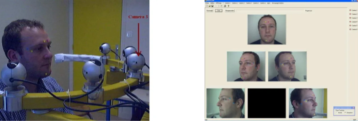
camera is fixed on a height-adjustable sliding support in order to adapt the camera position to each individual (see Figure 1 left). The acquisition program grabs images from the 5 cameras simultaneously (see Figure 1 right). These 5 images are stored in the PC with a frame data rate of 20×5 = 100 images per second.
The human subject sits in front of the acquisition system, directly facing the central camera (Camera 3). Different color markers are placed on the subject’s face. These markers are used later on to define common points between different face views. The position of these color markers corresponds roughly to the face fiduciary points. Figure 2 shows the position of the chosen points. There are 10 markers on each face with at least 3 markers in common between each face view.
Figure 1. The Acquisition system: the left panel shows the 5 cameras and their support, the right panel shows the five images collected from a subject. Each image size is240×320pixels.
With the cameras used, each pixel corresponds to a size of 1 mm2
. The area of each marker used is approximately 20 mm2
, which is sufficient for our application because it does not require a high precision (i.e., a precision of 1 mm in the marker position measurement is sufficient for our purposes).
Figure 2.Distribution of 10 markers in 5 views (clockwise from top left): Image 1, Image 2, Image 3, Image 4, and Image 5.
3. PANORAMIC FACE CONSTRUCTION
Several panoramic image construction algorithms have been already introduced20222324
.16
For example, Jain and Ross24
have developed an image mosaicing technique that constructs a more complete fingerprint template using two impressions of the same finger. In their algorithm, they initially aligned the two impressions using the corresponding minutiae points. Then, this
alignment was used by a modified version of the Iterative Closest Point (ICP) algorithm in order to compute a transformation matrix that defines the spatial relationship between the two impressions. A resulting composite image is generated using the transformation matrix which has 6 independent parameters: three rotation angles (α, β, γ) about the x, y, and z axes, respectively, and three translation components (tx, ty,tz) along the three axes. For faces,
Liu and Chen16
have proposed using facial geometry in order to improve the face mosaicing result. They used a spherical projection (instead of a cylindrical projection) because it works better with the head motion in both horizontal and vertical directions. A geometric matching algorithm has been developed in order to describe the correspondences between the 2D image plane space QU V and the spherical surface space Oαβ. In order to accomplish this, the two matching parameters [∆α,∆β]T are found using the Levenberg-Marquardt algorithm. In order
to improve the computational efficient, Liu and Chen approximated the mapping function with a triangular mesh, representing a face as a set of triangles.
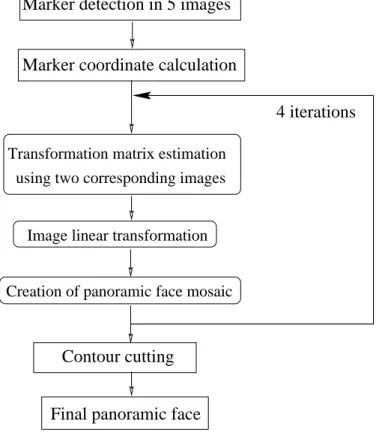
In general, the methods using non-linear transformations and iterative algorithms obtain very correct results in terms of geometric precision. However, these methods require a large number of computations and therefore cannot be easily implemented in real-time. Because we ultimately want to be able to build a real-time system, we decided to use simple (and therefore fast) linear methods. Our panoramic face construction algorithm is performed in three stages (see Figure 3):
1. Marker detection and marker coordinate calculation.
2. Transformation matrix estimation and image linear transformation. 3. Creation of panoramic face mosaics.
3.1. Marker detection and marker coordinate calculation
The first step of the algorithm corresponds to the detection of the markers put on the subject’s face. The markers were made of adhesive paper (so that they would stick to the subject’s face). We used 3 colors to create 10 markers (4 blue, 3 yellow, and 3 violet ones, see Figure 2 for an illustration). These three colors have been chosen after several tests because they are easily identifiable when compared to the face hue. These markers were used as reference points for pasting the different views of the face.
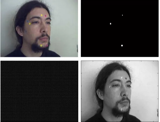
In order to detect the markers, we used color segmentation based upon the hue and saturation components of each image. This procedure allows a strong color selectivity and a small sensitivity to luminosity variation. Figure 4 illustrates the steps used for the yellow marker detection process. First, color segmentation gives, from the original image (Figure 4 top left), a binary image which contains the detected markers (Figure 4 top right). Then, in order to find the marker coordinates we used a logical AND operation which was performed between the binary image and a grid including white pixels separated by a fixed distance (Figure 4 bottom left). This distance has been chosen in relation to the marker area. A distance of 3 pixels allows us to capture all white zones (detected markers). Finally, we computed the centers of the detected zones (Figure 4 bottom right). These centers gives the coordinates of the markers in the image.
Final panoramic face
4 iterations Marker detection in 5 images
Marker coordinate calculation
Transformation matrix estimation using two corresponding images
Image linear transformation
Creation of panoramic face mosaic
Contour cutting
Figure 3. Block diagram of proposed panoramic face construction algorithm.
3.2. Transformation matrix estimation and image linear
transformation
We decided to represent each face as a mosaic. A mosaic face is a face made by concatenation of the different views pasted together as if they were on a flat surface. So, in order to create a panoramic face we combine the five different views. We start with the central view and paste the lateral views one at a time (see Figure 3). Our method consists of transforming the image to be pasted in order to link common points between this image and the target image. We obtain this transformed image by multiplying it by a linear transformation matrix. This matrix is calculated as a function of the coordinates of 3 common markers between 2 images. C1 and C2 represent, respectively, coordinates of the first and second images:
C1 = x1 x2 x3 y1 y2 y3 (1) C2 = x′ 1 x′2 x′3 y′ 1 y2′ y3′ (2) We obtain the transformation matrix as follows:
T=C1 ×(C⋆2)− 1
Figure 4. Yellow marker detection (reading left to right): original image, binary image after color filtering applied on Hue and Saturation components, a grid of white pixels, and marker coordinate localization. with C⋆2 = x′ 1 x′2 x′3 y′ 1 y2′ y3′ 1 1 1 (4) and T= a1 b1 c1 a2 b2 c2 (5) Then, we generalize this transformation to the whole image :
x=a1x′+b1y′+c1
y=a2x′+b2y′+c2
(6)
This linear transformation corresponds to a combination of image rotation, image transla-tion, and image dilation (see Figure 5). Figure 6 displays the superposition of Image 3 (not transformed) and Image 4 (transformed using the coordinates of the yellow markers as common points).
Figure 5.Image 4 before and after the linear transformation: the transformation matrix is computed using Image 4 and Image 3 (central view, see Figures 2 and 6).
Figure 6. Superposition of Images 3 and 4: original Image 3 (left), and superposition of transformed Image 4 and original Image 3 (right).
3.3. Creation of panoramic face mosaics
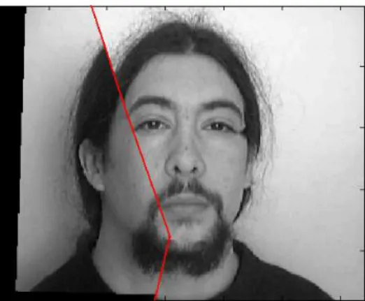
We begin the panoramic face construction with the central view (Image 3, see Figure 2). From the superposition of the original Image 3 and transformed Image 4 (see Figure 6), we remove redundant pixels in order to obtain a temporary panoramic 3-4 image (see Figure 7 left). In order to eliminate redundant pixels, we create a cutting line which goes through two yellow markers. This panoramic 3-4 image temporarily becomes our target image.
We repeat this operation for each view. First, Image 2 is pasted on the temporary panoramic Image 3-4 in order to obtain a new temporary panoramic 2-3-4 image (see Figure 7 right). The corresponding transformation matrix is generated using three common violet markers. Then, we compute the transformation matrix which constructs Image 2-3-4-5 (see Figure 8 left) using two blue markers and one yellow marker (topmost). Finally, Image 1 is pasted to the temporary panoramic Image 2-3-4-5 with the help of two blue markers and one violet marker (topmost) (see Figure 8 right).
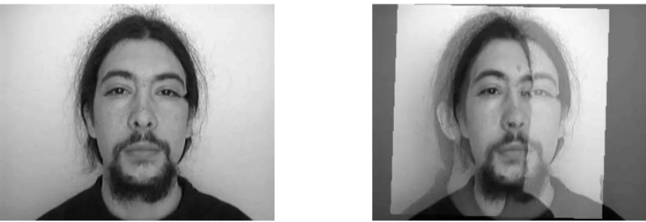
Figure 9 left displays the final panoramic face composition from 5 views. This composi-tion preserves some of the face shape. For example, the chin in a human face possesses more curvature than other parts, therefore the bottom part of the panoramic face is composed of 5
Figure 7. Mosaicing results: Image 3-4 (left), and Image 2-3-4 (right).
Figure 8. Mosaicing results: Image 2-3-4-5 (left), and Image 1-2-3-4-5 (right).
Figure 9. Mosaicing results: Panoramic face composition from 5 views (left), and final mosaic (right).
views: 1, 2, 3, 4, and 5. On the other hand, 3 views (1, 3, and 5) suffice to compose the top part. Figure 9 right shows the final mosaic face obtained after automatical contour cutting. For this, we first surround the panoramic face by a circle that passes by the extreme points of the ears in order to eliminate the background. Then, we replace segments of this circle by polynomial curves using extreme point coordinates located with the help of the marker positions.
Note that these 10 markers allow us to link common points between 5 views. The coordinates of the markers are computed in the marker detection process (see Section 3.1), and arranged in a table. Then, all 10 markers are erased from all 5 views using a simple image processing technique (local smoothing). This table of marker coordinates is regenerated for each temporary panoramic image construction. The goal of marker elimination is to use panoramic faces for face recognition or 3D face reconstruction applications.
As compared to the method proposed by Liu and Chen,16
panoramic faces obtained using our model are less precise in geometry. For example, Liu and Chen used a triangle mesh in order to represent a face. Each triangle possesses its proper transformation parameters. In our system, a single transformation matrix is generated for a complete image. Liu and Chen have also established a statistical modeling containing the mean image and a number of “eigen-images" in order to represent the face mosaic.
Our objective is to create a simple and efficient for later hardware implantations. Therefore, methods necessitating large amounts of computing time and a relatively large memory space are not adapted for the present objective. In order to test and validate our panoramic face mosaicing algorithm, we decided to use an approach based on the principal component analysis model originally proposed by Abdi,26
This method is described in the next section.
4. PANORAMIC FACE RECOGNITION
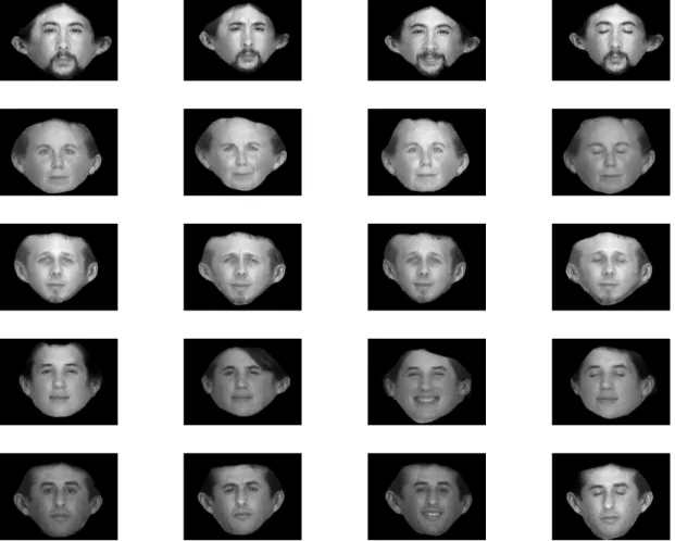
We created a panoramic face database using the method described in Section 3. This database is composed of 12 persons × 4 expressions × 2 sessions creating a total of 96 panoramic faces.
The two acquisition sessions were performed over an interval of one month. The four expressions were: neutral, smile, deepened eyebrows, and eyes closed (see Figure 10). We implemented a face recognition procedure using this database in order to validate our panoramic face mosaicing system.
4.1. Face recognition description : PCA
Over the past 25 years, several face recognition techniques have been proposed, motivated by the increasing number of real world applications and also by the interest in modeling human cognition. One of the most versatile approach is derived from the statistical technique called Principal Component Analysis (PCA) adapted to face images.25
Such an approach has been used, for example, by Abdi26
and Turk and Pentland4
for face detection and identification. PCA is based on the idea that face recognition can be accomplished with a small set of features that best approximates the set of known facial images. Application of PCA for face recognition proceeds by first performing a PCA on a well-defined set of images of known human faces (every person is represented by a number of different images, in which various expressions are captured). From this analysis, a set of L principal components is obtained and the projection of the new faces on these components is used to compute distances between new faces and old faces. These distances, in turn, are used to make predictions about the new faces (i.e., are these new or old faces?).
Figure 10. A sampling of panoramic faces from the first session’s database.
Technically, PCA on face images proceeds as follows. The K face images to be learned are represented by K vectors ak where k is the image number.27 Each vector ak is obtained
by concatenating the rows of the matrix storing the pixel values of the k-th face image. This operation is performed using the vec operation which transforms a matrix into a vector (see,21
for more details).
The complete set of patterns is represented by a I×K matrix notedA, whereI represents the number of pixels of the face images andK the total number of images under consideration. Specifically, the learned matrixA can be expressed as:
A=P∆QT (7)
where P is the matrix of eigenvectors of AAT, Q is the matrix of eigenvectors of ATA, and
∆ is the diagonal matrix of singular values of A, ∆ = Λ1/2 with Λ matrix of eigenvalues of
AAT and ATA. The left singular eigenvectorsP can be re-arranged in order to be displayed as images. In general, these images are somewhat face-like (26
) and are often called “eigen-faces" (4
Given the singular vectors P, every face in the database can be represented as a weight vector in the principal component space. The weights are obtained by projecting the face image onto the left singular vector, and this is achieved by a simple inner product operation (29
): P ROJx=xTP∆−1
(8) wherexis a face vector. It corresponds to a face exemplar in the training process or a test face in the recognition process. Therefore, when a new test image whose identification is required is given, its vector of weights also represents the new image. In general the number of pixels (I) is much larger than the number of face images (K) and therefore the number of singular vectors will be equal (at most) toK, which is also the dimension of the face weight vectors. Therefore, representing a face image by its weight vector corresponds to an important compression of the image.
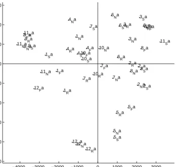
Identification of the test image is done by locating, in the known face database, the image which has the smallest Euclidean distance from the test image (the distances are computed from the weight vectors for greater computational efficiency). This algorithm is called “The nearest neighbor classification rule." Figure 11 displays the projections of the learned faces stored in matrix A on principal components 2 and 3. For this illustration, 48 panoramic faces were analyzed. Each panoramic face is labelled by its identity (12 persons, number 1-12), its expression (4 expressions coded N: neutral, S: smile, R: deepened, F: eyes closed) and its acquisition session (two sessions, a and b). Here only the first session (session a) is displayed.
−4000 −3000 −2000 −1000 0 1000 2000 3000 −5000 −4000 −3000 −2000 −1000 0 1000 2000 3000
Principal Component Number 2
Principal Component Number 3
1 Na 1 Ra 1 Sa 1 Fa 2 Na 2 Ra 2Sa 2 Fa 3 Na 3 Ra 3 Sa 3 Fa 4 Na 4 Ra 4 Sa 4 Fa 5 Na 5 Ra 5Sa 5 Fa 6 Na 6 Ra 6 Sa 6Fa 7Na 7Ra 7 Sa 7Fa 8 Na 8 Ra 8 Sa 8Fa 9 Na 9 Ra 9 Sa 9 Fa 10 Na 10Ra 10 Sa 10 Fa 11 Na 11 Ra 11 Sa 11Fa 12 Na12 Ra 12 Sa 12 Fa
PCA Space faces and expressions. Dimensions 2 and 3
Figure 11. 2D projection representation of learned matrix A on principal component 2 and 3; each panoramic face is differentiated by its identity (number 1-12), its expression (N,S,R,F), and its acqui-sition session (a, b).
5. EXPERIMENTAL RESULTS OF PANORAMIC FACE
RECOGNITION
5.1. Spatial representation
For these first tests, panoramic faces were analyzed using the original 240×320 pixel image
(spatial representation) without pre-processing. The database consisted of 12 persons × 4
expressions × 2 sessions = 96 panoramic faces, and was divided into two subsets. One subset
served as the face training set and the other subset provided the face testing test. As illustrated in Figure 10, all these panoramic faces possess a uniform background, and the ambient lighting varied according to the daylight.
From the panoramic face database, one, two, three, or four images were randomly chosen for each individual in order to create the training set (number of patterns for learning per individual p = 1,2,3,4). The rest of the panoramic faces were used in order to test the face recognition method. For example, when p = 1, the number of total training examples is equal to 1×12
persons =12, and the number of test samples for recognition is equal to96−12 = 84. Therefore,
for each individual, only one panoramic face is learned in order to recognize seven other images of this person. Several executions of our Matlab program were run for each value of p using randomly chosen training and testing sets. Then we computed mean performances, the results are presented in Table 1.
Using the nearest neighbor classification rule, the panoramic face identity test is done by locating the closest image in the known face database. Therefore, the system can make only confusion errors (i.e. associating the face of one person with a test face of another). In Table 1, the recognition rate corresponds to correct panoramic face recognition rate.
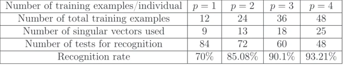
Table 1. Results of panoramic face recognition with spatial representation: the number of singular vectors used corresponds to the mean values obtained with the discriminant analysis algorithm during several executions.
Number of training examples/individual p= 1 p= 2 p= 3 p= 4
Number of total training examples 12 24 36 48 Number of singular vectors used 9 13 18 25 Number of tests for recognition 84 72 60 48
Recognition rate 70% 85.08% 90.1% 93.21%
We added a discriminant analysis stage in the face recognition process so as to determine the number of necessary eigenvectors. This analysis re-orders the eigenvectors, not according to their eigenvalues, but according to their importance for identification. Specifically, we computed the ratio of the between group inertia to the within group inertia for each eigenvector. This ratio expresses the quality of the separation of the identity of the subject performed by this eigenvector (a similar approach was taken by Abdi, Valentin, & O’Toole,5
and by O’Toole, Jiang, Abdi & Haxby, in press30
). The eigenvector with the largest ratio performs the best identity separation, the eigenvector with the second largest ratio performs second best, etc.
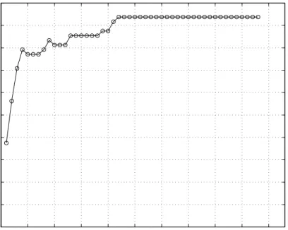
For the example shown in Figure 12, we observe that it suffices to use only 23 eigenvectors to reach the maximum recognition rate (93.75%). Additional eigenvectors do not add to the quality of the identification.
0 5 10 15 20 25 30 35 40 45 50 0 0.1 0.2 0.3 0.4 0.5 0.6 0.7 0.8 0.9 1
Number of Re−ordered eigenvectors
Recognition rate
Figure 12. Recognition rate in function of the number of re-organized eigenvectors. 5.1.1. Frequential representation
We also tested our recognition system in term of spatial frequencies. Figure 13 left displays the FFT amplitude of a panoramic face. We can observe that spectrums are well centered in low frequencies. This allows us to apply a low-pass filter in order to reduce the size of the data to process (see Figure 13 right). Only 80×80FFT amplitude values of low frequencies were used
for the recognition system.
Figure 13. Original FFT amplitude 3D representation (left), and low frequencies, FFT amplitude of only80×80 = 6400values which are presented to the recognition system (right).
We applied the same training and testing process as used in spatial representation. Test results are given in Table 2. We obtain a better recognition rate with the frequential representa-tion (97.46%) than with the spatial representarepresenta-tions (93.21%). This advantage of the frequencial representation is due to the fact that for face images, the spectrum amplitude is less sensitive to noise (or variations) than the spectrum phase. We confirmed this interpretation by using a panoramic face image to which noise was added. Figure 14a shows a original panoramic face. Figure 14b displays the same panoramic face image with added noise. We first performed the FFT of these two images and, then their inverse FFT in the two following manners:
1. Using the spectrum amplitude of the noised image and the spectrum phase of the original image (see Figure 14c).
2. Using the spectrum phase of the noised image and the spectrum amplitude of the original image (see Figure 14d).
These results show that the face obtained with the first configuration is closer to the original face than the face obtained with the second configuration. This confirms that the spectrum amplitude is less sensitive to noise than the spectrum phase.
Table 2. Results of panoramic face recognition with frequential representation
Number of training examples/individual p= 1 p= 2 p= 3 p= 4
Number of total training examples 12 24 36 48 Number of singular vectors used 8 13 18 24 Number of test for recognition 84 72 60 48
Recognition rate 76.83% 91.26% 93.25% 97.46%
5.1.2. Discussion
Tsalakanidou et al.8
described a study designed to evaluate three different approaches (color, depth, combination of color and depth) for face recognition and quantity the contribution of depth. The color images were stored in portable pixmap format (ppm) with a resolution of
720 ×576 pixels. In addition, for each person the “structured light" approach was used for
capturing the 3D facial surface and thus creating the depth map. Their experimental results show significant gains of 5% with the use of depth information. They have obtained a recognition rate of 97.5% using the depth map and color frontal view. The face recognition technique used is based on the implementation of the PCA algorithm (similar to ours). How does our system compare with these results? By using a simple and easily built system, we were able obtain some 3D face information, and we obtained performance levels of panoramic face recognition very close to those reported by Tsalakanidou etal..
Figure 14. Amplitude is less sensitive to noise than phase (from left to right, top to bottow): a).
An original panoramic face image; b). Original image with added Gaussian noise (mean=0 and vari-ance=0.05); c). IFFT image using the spectrum amplitude of b) and the spectrum phase of a); and
d). IFFT image using the spectrum amplitude of a) and the spectrum phase of b). The image c) is more similar to the imagea)than the imaged).
5.2. Panoramic face recognition with negative samples
In order to evaluate the behavior of our system for unknown people, we added 4 people to the test database (see Figure 15). These panoramic faces were obtained as described in Section 3.
Figure 15. Panoramic faces of four unknown persons.
Table 3 displays different test performances. We added 4 persons×4 expressions×2 sessions = 32 panoramic faces in each test set. In order to reject these unknown faces, we established a threshold of Euclidean distance. Because we are working on applications of typical access control, where confusion is more harmful than non-recognition, we decided to use a relatively severe acceptance threshold in order to reject intruders. Note that the acceptance threshold is constant for all tests. Efficiency is defined as follows:
Recognition: correct recognition of a panoramic face,
Non-recognition: a panoramic face has not been recognized,
Confusion: a panoramic face is confused with an intruder.
Table 3.Results of panoramic face recognition with negative samples: these performances were obtained using the frequential representation. Performance declined in comparison with tests without negatives samples.
Number of training examples/individual p= 1 p= 2 p= 3 p= 4
Number of total training examples 12 24 36 48 Number of singular vectors used 8 13 18 24 Number of tests for recognition 116 104 92 80
Non-recognition rate 25.4% 12.74% 7.58% 4.82%
Confusion rate 5.85% 4% 3.5% 2.8%
Recognition rate 68.75% 83.26% 88.92% 92.38%
6. CONCLUSIONS AND PERSPECTIVES
In this paper, we proposed a fast and simple method for panoramic face mosaicing. The ac-quisition system consists of several cameras, and uses a series of fast linear transformations of the images produced by t he cameras. The simplicity of the computations makes it possible to envisage real-time applications.
In order to test the recognition performance of our system, we used the panoramic faces as in-put to a recognition system based upon principal component analysis. We tested two panoramic face representations: spatial and frequential. We found that a frequential representation gives the best performance with a correct recognition rate of 97.46% versus 93.21% for spatial rep-resentation. An additional advantage of the frequential representation is to reduce the data volume to process and this further accelerates calculation speed. We used negative samples for panoramic face recognition system and the correct recognition rate was 92.38%. Experimental results show that our fast mosaicing system provides relevant 3D facial surface information for recognition application. Obtained performance is very close or superior to published levels623
.8
In the future, we plan to simplify our acquisition system by replacing the markers by a structured light. We also hope to use our system without markers. For this, we will detect control points on faces (corners and maximum curvature ...). Another line of development is to improve the geometry quality of our panoramic face mosaic construction16
.31
For this, we will use realistic human face models. We are also exploring processing panoramic face recognition using others classifiers with more variable conditions. Then, 3D face applications are envisaged such as real time human expression categorization using movement estimation and fast 3D facial modeling for compression and synthesis such as in video-conferencing.
REFERENCES
1. S.Y. Kung, M.W. Mak and S.H. Lin, Biometric authentification: A machine learning approach, Prentice-Hall, Supper Saddle River (NJ), 2005.
2. A.J. Howell and H. Buxton,Learning identity with radial basis function networks, Neurocomputing, Vol.20, pp.15-34, 1998.
3. T. Sim, R. Sukthankar and al.,Memory-Based face recognition for visitor Identification, 4th IEEE International Conf. On automatic face and gesture recognition, Grenoble, France, 26-30 March 2000. 4. M. Turk and A. Pentland, Eigenfaces for recognition, Journal Cognitive neuroscience, Vol.3,
pp.71-86, 1991.
5. H. Abdi, D. Valentin and A. O’Toole,A generalized auto-associator model for face semantic process, inOptimization and neural network, edited by D.Levine (Erlbaum, Hillsdale), 1997.
6. M. Slimane, T. Brouard andal.,Unsupervised learning of pictures by genetic hibrydization of hidden Markov chain, Signal Processing, Vol.16, No.6, pp.461-475, 1999.
7. P.J. Phillips, P. Grother and al.,Face recognition Vendor Test 2002, IEEE International workshop on Analysis and Modeling of Faces and Gestures (AMFG), 2003.
8. F. Tsalakanidou, D. Tzovaras and M.G. Strintzis, Use of delth and colour eigenfaces for face recog-nition, Pattern recognition Letters, Vol.24, pp.1427-1435, 2003.
9. C. Beumier, M. Acheroy, Face verification from 3D and grey level clues, Pattern recognition letters, Vol.22, pp.1321-1329, 2001.
10. C. Hehser, A. Srivastava and G. Erlebacher, A nouvel technique for face recognition using range imaging, 7th International Sympoosium on Siganl Processing and its Apllications (ISSPA), 2003. 11. X. Lu, D. Colbry and A.K. Jain, Three-Dimensional model based face recognition, Proc.
Interna-tional Conference on Pattern Recognition, Cambridge, UK, August, 2004.
12. K.W. Bowyer, K. Chang and P. Flynn, A survey of 3D and multi-modal 3D+2D face recognition, International Conference on Pattern Recognition (ICPR), 2004.
13. V. Blanz and T. Vetter, Face recognition based on fitting a 3D morphable model, IEEE Transaction on Pattern Analysis and Machine Intelligence, Vol.25, pp.1063-1074, September, 2003
14. J.G. Wang, R. Venkateswarlu and E.T. Lim, Face tracking and recognition from stereo sequence, Computer Science, Vol. 2688, pp.145-153, 2003.
15. R. Hartly and A. Zisserman, Multiple View Geometry in Computer vision, Cambridge University Press, Second Edition, 2003.
16. X. Liu and T. Chen, Geometry-assisted statistical modeling for face mosaicing, IEEE International Conference on Image Processing (ICIP), Vol.2, pp.883-886, Barcelona, Spain, 2003.
17. F. Yang, M. Paindavoine, and H. AbdiA new filtering technique combining a wavelet transform with a linear neural network: application to face recognition, Optical Engineering SPIE. Vol.39, No.11, 2000.
18. J. Mitéran, J.P. Zimmer, F. Yang and M. Paindavoine, Access control: adaptation and real time implantation of a face recognition method, Optical Engineering SPIE. Vol.40, No.4, 2001.
19. F. Yang, M. Paindavoine, Implementation of a RBF neural network on embedded systems: Real time face tracking and identity verification, IEEE Transactions on Neural Networks, Vol.14, No.5, pp.1162-1175, September 2003.
20. Y. Kanazawa and K. Kanatani, Image mosaicing by stratified matching, Image and Vision comput-ing, Vol.22, pp.93-103, 2004.
21. H. Abdi, D. Valentin, B.E. Edelman, A.J. O’Toole. More about the difference between men and women: Evidence from linear neural networks and the principal component approach. Perception, Vol.24, 539–562, 1995.
22. Y. Zhou, H. Xue and M. Wan, Inverse image alignment methode for image mosaicing and video stabilization in fundus indocyanine green angiography under confocal scanning laser ophthalmoscope, Computerized Medical Imaging and Graphics, Vol.27, pp.513-523, 2003.
23. P.F. McLauchlan and A. Jaenicke,Image mosaicing using sequential bundle adjustment, Image and Vision computing, Vol.20, pp.751-759, 2002.
24. A.K. Jain and A. Ross,Fingerprint Mosaicing, IEEE International Conference on Acoustics, Speech, and Signal Processing (ICASSP), Orlando, Florida, May, 2002.
25. D. Valentin, H. Abdi, A.J. O’Toole and G.W. Cottrell, Connectionist models of face processing: A survey, Pattern Recognition, Vol.27, 1208-1230, 1994.
26. H. Abdi, A generalized approach for connectionist auto-associative memories: interpretation, im-plications and illustration for face processing. In J. Demongeot (Ed.), Artificial Intelligence and Cognitive Sciences. Manchester: Manchester University Press, (1988).
27. H. Abdi, D. Valentin and B. Edelman,Neural Networks, Sage, Thousand Oaks, 1999.
28. M.C.K. Yang and D.H. Robinson,Understanding and learning statistics by computer, World Scien-tific, Singapore, 1986.
29. H. Abdi,Linear algebra for neural networks inInternational Encyclopedia of the Social and Behav-ioral Sciences, edited by N.J. Smelser, P.B. Baltes (Elsevier, Oxford), 2001.
30. A.J. O’Toole, F. Jiang, H. Abdi and J.V. Haxby,Partially distributed representations of objects and faces in ventral temporal cortex, Journal of Cognitive Neuroscience, Vol.17, (in press, 2005). 31. W. Puech, A.G. Bors and al., Projection distortion analysis for flattened image mosaicing from
Fan Yang received a B.S degree in eletrical engineering from the University of Lanzhou (China) in 1982. She was a Scientific Assistant at the Departement of electronics in the University of Lanzhou. She received an M.S. (D.E.A.) degree in computer science and a Ph.D. degree in image processing from the University of Burgundy (France), respectively in 1994 and in 1998. She is currently an Associate Professor and member of LE2I CNRS-UMR (Laboratory of Electronic, Computing and Imaging Sicences). Her research interests are in the areas of patterns recognition, neural network, motion estimation based on spatio-temporal Gabor filters, parallelism and real-time implementation, and more specifically, automatic face image processing: algorithms and architectures.
Michel Paindavoine received a Ph.D. in Electronics and Signal Processing from the Montpellier University, France 1982. He was with Fairchild CCD company for two years as engineer special-ized on CCD sensors. He joined the Burgundy University in 1985 as "Maitre de Conferences" and is currently full professor and director of LE2I UMR-CNRS, Laboratory of Electronic, Com-puting and Imaging Sicences, Burgundy University, France. His main research topics is image acquisition and real time image processing. He is also a member of ISIS (a resarch group in Signal and Image Processing of the French National Scientific Research Committee).
Hervé Abdi received an M.S. in Psychology from the University of Franche-Comté (France) in 1975, an M.S. (D.E.A.) in Economics from the University of Clermond-Ferrand (France) in 1976, an M.S. (D.E.A.) in Neurology from the University Louis Pasteur in Strasbourg (France) in 1977, and a Ph.D. in Mathematical Psychology from the University of Aix-en-Provence (France) in 1980. He was an assistant professor in the University of Franche-Comté (France) in 1979, an associate professor in the University of Bourgogne at Dijon (France) in 1983, a full professor in the University of Bourgogne at Dijon (France) in 1988. He is currently a full professor in the school of behavioral and brain sciences at the University of Texas at Dallas. He was twice a Fulbright scholar and was a visiting professor in Brown University, and the Universities of Dijon (France), Chuo (Japan), and Geneva (Switzerland). His interest includes neural networks and cognitive modeling, experimental design, multivariate statistics, and data analysis of large data sets (such as brain imaging).
List of Tables
1 Results of panoramic face recognition with spatial representation: the number of singular vectors used corresponds to the mean values obtained with the discrimi-nant analysis algorithm during several executions. . . 12 2 Results of panoramic face recognition with frequential representation . . . 14 3 Results of panoramic face recognition with negative samples: these performances
were obtained using the frequential representation. Performance declined in com-parison with tests without negatives samples. . . 16
List of Figures
1 The Acquisition system: the left panel shows the 5 cameras and their support, the right panel shows the five images collected from a subject. Each image size is 240×320 pixels. . . 3
2 Distribution of 10 markers in 5 views (clockwise from top left): Image 1, Image 2, Image 3, Image 4, and Image 5. . . 3 3 Block diagram of proposed panoramic face construction algorithm. . . 5 4 Yellow marker detection (reading left to right): original image, binary image after
color filtering applied on Hue and Saturation components, a grid of white pixels, and marker coordinate localization. . . 6 5 Image 4 before and after the linear transformation: the transformation matrix is
computed using Image 4 and Image 3 (central view, see Figures 2 and 6). . . . 7 6 Superposition of Images 3 and 4: original Image 3 (left), and superposition of
transformed Image 4 and original Image 3 (right). . . 7 7 Mosaicing results: Image 3-4 (left), and Image 2-3-4 (right). . . 8 8 Mosaicing results: Image 2-3-4-5 (left), and Image 1-2-3-4-5 (right). . . 8 9 Mosaicing results: Panoramic face composition from 5 views (left), and final
mosaic (right). . . 8 10 A sampling of panoramic faces from the first session’s database. . . 10 11 2D projection representation of learned matrixAon principal component 2 and 3;
each panoramic face is differentiated by its identity (number 1-12), its expression (N,S,R,F), and its acquisition session (a, b). . . 11 12 Recognition rate in function of the number of re-organized eigenvectors. . . 13 13 Original FFT amplitude 3D representation (left), and low frequencies, FFT
am-plitude of only 80× 80 = 6400 values which are presented to the recognition
system (right). . . 13 14 Amplitude is less sensitive to noise than phase (from left to right, top to bottow):
a). An original panoramic face image; b). Original image with added Gaussian noise (mean=0 and variance=0.05); c). IFFT image using the spectrum ampli-tude ofb)and the spectrum phase ofa); andd). IFFT image using the spectrum amplitude of a) and the spectrum phase of b). The image c) is more similar to the image a) than the image d). . . 15 15 Panoramic faces of four unknown persons. . . 15