A Partial-Closure Canonicity Test to Increase the Efficiency
of CbO-Type Algorithms
ANDREWS, Simon <http://orcid.org/0000-0003-2094-7456>
Available from Sheffield Hallam University Research Archive (SHURA) at:
http://shura.shu.ac.uk/8607/
This document is the author deposited version. You are advised to consult the
publisher's version if you wish to cite from it.
Published version
ANDREWS, Simon (2014). A Partial-Closure Canonicity Test to Increase the
Efficiency of CbO-Type Algorithms. In: HERNANDEZ, Nathalie, JÄSCHKE, Robert
and CROITORU, Madalina, (eds.) Graph-Based Representation and Reasoning.
Lecture Notes in Computer Science (8577). Springer, 37-50.
Copyright and re-use policy
See
http://shura.shu.ac.uk/information.html
Sheffield Hallam University Research Archive
A partial-closure canonicity test to increase the
efficiency of CbO-type algorithms
Simon Andrews
Conceptual Structures Research Group Communication and Computing Research Centre Faculty of Arts, Computing, Engineering and Sciences
Sheffield Hallam University, Sheffield, UK
Abstract. Computing formal concepts is a fundamental part of Formal Concept Analysis and the design of increasingly efficient algorithms to carry out this task is a continuing strand of FCA research. Most ap-proaches suffer from the repeated computation of the same formal con-cepts and, initially, algorithms concentrated on efficient searches through already computed results to detect these repeats, until the so-called canonicity test was introduced. The canonicity test meant that it was sufficient to examine the attributes of a computed concept to determine its newness: searching through previously computed concepts was no longer necessary. The employment of this test in Close-by-One type al-gorithms has proved to be highly effective. The typical CbO approach is to compute (close) a concept and then test its canonicity. This pa-per describes a more efficient approach, whereby a concept need only be partially closed in order to carry out the test. Only if it passes the test does its closure need to be completed. This paper presents this partial-closure canonicity test in the In-Close algorithm and compares this to a traditional CbO algorithm to demonstrate the increase in efficiency.
Keywords: Formal Concept Analysis; FCA; FCA algorithms; Com-puting formal concepts; Canonicity test; Partial-closure canonicity test; Close-by-One; In-Close; CbO
1
Introduction
‘canonicty test’ [11], whereby the attributes concept could be examined to de-termine its uniqueness in the computation. This test has given rise to a number of algorithms based on the Close-by-One (CbO) algorithm [19] and the focus of research has been to develop improvements of the original CbO algorithm. This paper presents one such improvement in the form of a more efficient canonicity test: the partial-closure canonicity test.
The next two sections of the paper briefly describe formal concepts and the main issues involved in their efficient computation, showing how testing a com-puted concept’s canonicity is an efficient means of detecting the computation of repeated results. Section 4 shows a CbO algorithm incorporating a canonicity test that involves the full closure of concept before testing. Section 5 presents a partial-closure canonicity test that avoids the need for full closure before testing and in Section 6 the partial-closure test is realised in the In-CloseI algorithm. Section 7 compares and evaluates the efficiency of the algorithms by carrying out ‘level playing field’ implementations and experiments on variety of data sets. Another recent advance in CbO-type algorithms, that allows the inheritance of failed canonicity tests in the recursion, is included in the evaluations. Finally, the paper makes its conclusions and suggestions for further work in Section 8.
2
Formal Concepts
A description of formal concepts [12] begins with a set of objectsX and a set of attributes Y. A binary relation I ⊆ X ×Y is called the formal context. If x ∈ X and y ∈ Y then xIy says that object x has attribute y. For a set of objectsA⊆X, a derivation operator↑ is defined to obtain the set of attributes
common to the objects in Aas follows:
A↑:={ y∈Y | ∀x∈A:xIy}. (1) Similarly, for a set of attributesB ⊆Y, the ↓ operator is defined to obtain
the set of objects common to the attributes in B as follows:
B↓:={x∈X | ∀y∈B:xIy}. (2)
(A, B) is a formal concept iff A↑ = B and B↓ =A. The relations A×B
are then a closed set of pairs in I. In other words, a formal concept is a set of attributes and a set of objects such that all of the objects have all of the attributes and there are no other objects that have all of the attributes. Similarly, there are no other attributes that all the objects have. A is called the extent of the formal concept andB is called theintent of the formal concept.
A formal context is typically represented as a cross table, with crosses in-dicating binary relations between objects (rows) and attributes (columns). The following is a simple example of a formal context:
0 1 2 3 4
a × × ×
b × × × × c × ×
Formal concepts in a cross table can be visualised as closed rectangles of crosses, where the rows and columns in the rectangle are not necessarily con-tiguous. The formal concepts in the example context are:
C1= ({a, b, c, d},∅) C6 = ({b},{1,2,3,4}) C2= ({a, c},{0}) C7 = ({b, d},{1,2,4}) C3= (∅,{0,1,2,3,4})C8 = ({b, c, d},{2}) C4= ({c},{0,2}) C9 = ({a, b},{3,4}) C5= ({a},{0,3,4}) C10= ({a, b, d},{4})
3
Computation of formal concepts
A formal concept can be computed by applying the ↓ operator to a set of
at-tributes to obtain its extent, and then applying the↑ operator to the extent to
obtain the intent. This is the notion of concept closure. For example, taking an arbitrary set of attributes, say{1,2}, from the the context above,{1,2}↓={b, d}
and {b, d}↑ ={1,2,4}. ({b, d},{1,2,4}) is concept C7 in the list above. If this
procedure is applied to every possible combination of attributes, then all the concepts in the context will be computed.
Thus, if there arenattributes in a formal context there are, potentially, 2n
concepts. It is the exponential nature of the problem that provides the com-putational challenge, compounded by the fact that the same concept can be computed more than once - in the worst case, exponentially many times. For ex-ample, in the context above, the conceptC7will be computed six times because
the extent{b, d} can be obtained from the closure of six different combinations of attributes:{b, d}={1}↓={1,2}↓={1,2,3}↓={1,4}↓={2,4}↓={4}↓.
Thus determining that a concept is a repeat is a key halting condition of the algorithm if we are only interested in obtaining unique concepts. The algorithm
ComputeConceptsOnce, below, illustrates this approach by intersecting a current extentAwith successive attribute closures (successive ‘columns’ in the context), closing the resulting ‘candidate’ new extent C and then testing the newness of the resulting concept. If the concept passes the test it is processed in some way (stored for example) and the algorithm called again, passing the new extent and the next attribute to the next level of recursion. The algorithm is invoked with an extent and a starting attribute, initially (X,0).
ComputeConceptsOnce(A, y)
forj←y upton−1do C←A∩ {j}↓
B←C↑
if NewConcept(C, B)then
ProcessConcept(C, B)
Early algorithms concentrated on finding repeats by efficiently searching the previously generated concepts. Lindig’s algorithm [23], and others like it, use a search tree to quickly find repeated results. Others use a hash function where the cardinality of results is used to divide them into groups, thus narrowing the search [13]. The problem with these approaches is that even an efficient search becomes expensive when there is a large number of repeated concepts.
Ganter noticed [11] that the basic algorithm recursively iterated attribute combinations in the natural combinatorial order, or canon. A concept is thus canonical if, when it is computed, its rank comes after the previous canonical concept. For example, the concepts in Section 2, above, are listed in the nat-ural combinatorial order of their intents: ∅ < {0} < {0,1,2,3,4} < {0,2} <
{0,3,4} <{1,2,3,4}, and so on. If the previous concept to be computed had the intent {0,3,4} and the next concept had the intent {0,2}, it would be re-jected as a repeat: it will have been generated earlier in the computation. It is this canonicity, and the testing thereof, that has become fundamental in detecting the repeated computation of a concept. If concepts are computed in this order, then if a concept is generated that has a rank lower or equal to that of its predeces-sor, it must be a repeat. Kuznetsov specified in Close-by-One (CbO) [19, 21] an efficient means of achieving this with a time complexity ofO(|G||M|2|L|), where
L is the set of concepts, or O(|M|2|G||L|) if the main cycle of the algorithm is
over attributes instead of objects, as in the CbO-type algorithms presented here. CbO has thus formed the basis for several variants and improvements [1, 2, 16, 17, 26] and it has been shown, in numerous tests, that these CbO-type algorithms are significantly faster than previous algorithms [1, 2, 6, 15–17, 22, 26, 28], outperforming algorithms including Chein [9], Norris [24], Next-Closure [11], Bordat [7], Godin [13], Nourine [25] and Add-Intent [30].
4
CbO Algorithm [16]
In the CbO algorithm of Krajca, Outrata and Vychodil [16], the canonicity test for a new concept is carried out by comparing a newly computed intent,D, with its predecessor, B. If they agree in all attributes up to the current attribute,j, then the new concept is canonical. If, however, there is an attribute inDthat is not inBand that comes beforej then the concept is not canonical (it will have been computed earlier). Thus a new concept is canonical if:
B∩Yj=D∩Yj (3)
WhereYj is the set of attributes up to but not includingj:
Yj:={y∈Y |y < j} (4)
The algorithm is written below and is called ComputeConceptsFrom. The
procedure is invoked with the initial concept (A, B) = (X, X↑) and attribute
y= 0.
CbO
ComputeConceptsFrom((A, B), y)
ProcessConcept((A, B))
1
forj←y upton−1do
2
if j /∈B then
3
C←A∩ {j}↓
4
D←C↑
5
if B∩Yj=D∩Yjthen
6
ComputeConceptsFrom((C, D), j+ 1)
7
A line-by-line explanation of the algorithm is as follows:
Line 1 - Pass concept (A, B) to notional procedureProcessConceptto pro-cess it in some way (for example, storing it in a set of concepts).
Line 2 - Iterate across the context, from attributey up to attributen−1. Line 3 - Test if the next attribute is in the current intent,B. If it is, skip it to avoid computing the same concept again.
Line 4 - Otherwise, form an extent,C, by intersecting the current extent,A, with the next column of objects in the context.
Line 5 - Close the extent to form an intent,D. Thus the concept (C, D) is computed (‘fully closed’) before the canonicity test is carried out to determine if it is a new one:
Line 6 - Perform the canonicity test by checking that attributes inBandD agree up to the current attribute. If they do then the concept (C, D), is a new one so:
Line 7 - Recursively compute concepts from the new one, starting from the next attribute in the context.
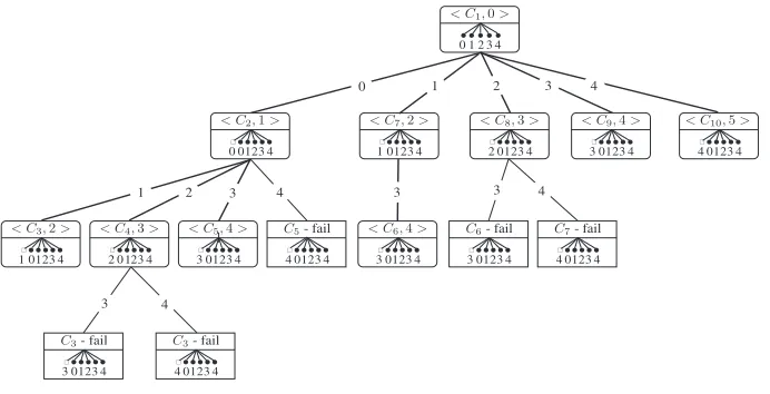
CbO call tree- Figure 1 shows the CbO call tree for the simple example. A rounded box represents the computation of a concept and a square box represents the computation of a repeated concept (that then fails the canonicity test). The lower part of a box shows the intersections carried out in the computation of the corresponding concept: the empty-square arrows are the extent intersections, A∩ {j}↓, and the filled-circle arrows are the closure intersections inC↑. In each case the number pointed to represents the attribute involved. Note that each concept, new or repeat, requires a full closure. The notation< Cx, j >represents
There are a total of 15 closures in the tree, with five intersections required for each closure, plus 14 extent intersections, making a total of 89 intersections for CbO.
1 2 3 4
1 2 3 4 3 4
3 4
3 0
< C1,0>
< C2,1> < C7,2> < C8,3> < C9,4> < C10,5>
< C3,2> < C4,3> < C5,4> < C6,4> 2 1 3 0 ! " 4
0 0123
! " 4 2 2 13 0 ! " 4
1 0123
!
"
4
3 0123
! " 4 4 2 1 3 0 ! " 4
1 2!"01234 3!"01234 4!"01234 3!"01234 3"!01234 4!"01234
2 13 0 ! " 4
3 4!"01234
2 3 4 1 0
C3- fail C3- fail
[image:7.612.137.483.171.348.2]C5- fail C6- fail C7- fail
Fig. 1.CbO Call Tree
5
A partial-closure canonicity test
In the CbO algorithm, above, a concept is fully closed before the canonicity test is applied to it. However, it is sufficient to close a concept only up to the current attribute j to determine its canonicity. Remember that the canonicity test in CbO compares the previous and new intent to see that they agree in all attributes up to the current attribute. Attributes after the current one have no bearing on the canonicity.
Thus in designing a partial-closure canonicity test we define, from 1 and 4, a partial-closure operator↑j as a modification of the original closure operator:
A↑j :={y∈Y
j | ∀x∈A:xIy}. (5)
The partial-closure canonicity test will thus determine if the attributes in the intentB, up toj, agree with the attributes in the closure of C up toj and can be defined from 5 and 3 as:
B∩Yj=C↑j (6)
If there is an attribute inC↑j that is in B beforej then the concept is not
canonical and is a repeat.
The efficiency is that a partial-closure,C↑j, is clearly less expensive to
of intersections equal to the number of attributes, n, whereas the cost of the partial-closure is always< n.
In fact, the implementation of the partial closure test can be even more efficient because the closure can be haltedas soon as an attribute is found that is in B before j, so the cost of the closure will actually be < j for each test failure.
Of course, if the canonicity test is passed, new concepts still need to be fully closed and this can be carried out in the In-Close type of CbO algorithms.
6
In-CloseI algorithm with partial-closure test
This section gives an updated version of the algorithm given in [1]. The key difference to the CbO algorithm in Section 4, above, is that the canonicity test is appliedbeforea concept is fully closed. The closure of a concept that passes the test is completed at the next level of recursion, by adding the current attributej to the intentBwhenever the current extentAis found: i.e. wheneverA∩ {j}↓=
A. This test of equality can be implemented with almost zero additional cost, given that the intersectionA∩ {j}↓is carried out in any case. Whenever a new
concept is detected, the current, partial, intent is passed to the next level. The intent is then fully closed when the main cycle at the next level is completed.
The algorithm, given asIn-CloseIbelow, is invoked with the initial concept (A, B) = (X,∅) and initial attributey= 0.
In-CloseI
ComputeConceptsFrom((A, B), y)
forj←y upton−1do
1
C←A∩ {j}↓
2
if A=Cthen
3
B←B∪ {j}
4
else
5
if B=C↑j then 6
D←B∪ {j}
7
ComputeConceptsFrom((C, D), j+ 1)
8
ProcessConcept((A, B))
9
Line 1 - Iterate across the context, from starting attributeyup to attribute n−1.
Line 2 - Form an extent, C, by intersecting the current extent,A, with the next column of objects in the context.
Line 4 - ...add the current attributej to the intent being closed,B.
Line 6 - Otherwise the new partial-closure canonicity test is applied. A small simplification to the canonicity test can be made becauseB is being completed incrementally withj. In other words, at the time of the test,B=Bj=B∩Yj.
Therefore, in the canonicity test, B ∩Yj can be replaced with B. So if the
attributes inB agree with those in the partial-closureC↑j the extent must be a
new one so...
Line 7 - Create a new partial intentD that inherits the attributes ofB, plus the current attributej.
Line 8 - Pass the new extent C, the partial intentD and the next location j+ 1 to the next level so that concepts from there can be computed and so that the closure ofD can be completed.
Line 9 - Pass concept (A, B) to notional procedureProcessConceptto pro-cess it in some way (for example, storing it in a set of concepts). Note that in In-Close this happens at the end of the procedure, once the main cycle has completed the closure of the intent,B.
Correctness of In-CloseI- CbO and In-CloseI use the same cycle to form the same extents,C. The only pertinent difference up to this point is the skipping of attributes in CbO when j ∈B (Line 3). However, this test is only to avoid forming an extent that will fail the canonicity test anyway. Thus to show that In-CloseI is correct it is sufficient to show that the partial-closure canonicity test is equivalent to the original test, in other words, given the same extentC, show that the tests produce the same result:
(B=C↑j)≡(B∩Y
j=D∩Yj)
As previously stated, in In-CloseI the intentB is incrementally closed up to the current attributej, thusB=B∩Yj, so it is sufficient to show that:
C↑j ≡D∩Y j
ReplacingDwithC↑, from Line 5 of CbO:
C↑j ≡C↑∩Y j
Thus, from (1) and (5):
{y∈Yj | ∀x∈C:xIy} ≡ {y∈Y | ∀x∈C:xIy} ∩Yj.
So on the left side are all the attributes up tojthat are related to the extent and on the right are all the attributes that are related to the extent, intersected with all the attributes up to j. Both sides are thus clearly equivalent.
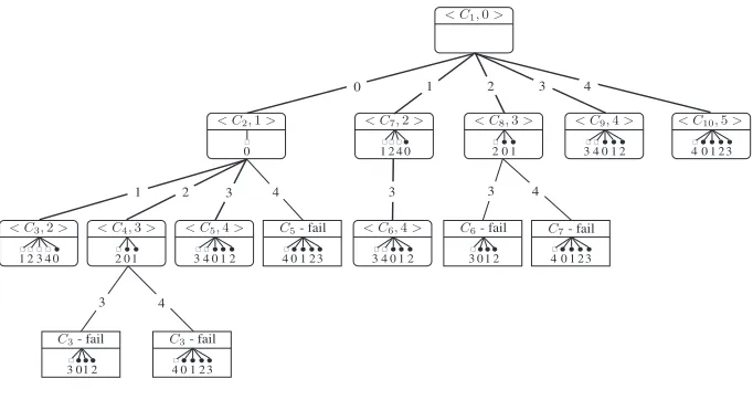
then fails the canonicity test). The notation < Cx, j > is the invocation of the
next level in the form of concept (extent and partial intent) and corresponding initial attribute. The numbered lines connecting the boxes represent the iteration ofj in the main cycle.
The computations are now partial with intents being completed at the next level. The lower part of a box, as in the CbO tree, shows the intersections carried out in the computation of the corresponding concept: the empty-square arrows are the extent intersectionsA∩ {j}↓ and the filled-circle arrows are the closure
intersections inC↑j. In each case the number pointed to represents the attribute
involved. Note that, now, each concept is closed only up toj. Thus the In-Close call tree shows fewer closure intersections than CbO. If the canonicity test is passed the intent is closed at the next level, requiring some additional extent intersections. Altogether there are 59 intersections in the tree, 30 fewer than for CbO.
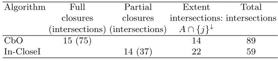
Table 1 summarises the performance of each algorithm using the simple con-text example from Section 2. The table counts and compares the number of full and partial-closures and the number of extent intersections, A∩ {j}↓. Because
closure itself involves repeated intersections of an extent with columns of the context, it is convenient to use the intersection as a measure of performance. For a full closure,C↑, there arenintersections (in the example,n= 5) and for a partial-closure, C↑j, there arej−1 intersections. To perform the evaluation
and create the call-trees, a paper run of each algorithm was carried out, line by line. These are too lengthy to be presented here but are available as an on-line appendix [3].
1 2 3 4
1 2 3 4 3 4
3 4
3 0
< C1,0>
< C2,1> < C7,2> < C8,3> < C9,4> < C10,5>
< C3,2> < C4,3> < C5,4> < C6,4>
C3- fail
0 24
! 0 1 ! " 0 1 2
!! " 0 1 2 4 3
! " " " 1 23 0 4
3 4 0 2 1
!! " 0 1 2 4 3 ! "
01 2
!" " " 1 23 0 4
!! " 0 1 2 4 3 "" 1 0 ! 2 3
!" " " 1 23 0 4 "" 1 0 ! 2 3
C3- fail
C5- fail C6- fail C7- fail
! ! ! ! " " " " " " " " "
! !!" " " "
!" " " 1 23 0 4 "
"
[image:10.612.138.479.432.613.2]"
Table 1.Comparison of closures and intersections for the simple context example
Algorithm Full Partial Extent Total
closures closures intersections: intersections
(intersections) (intersections) A∩ {j}↓
CbO 15 (75) 14 89
In-CloseI 14 (37) 22 59
7
Performance Evaluation
7.1 Incorporating the partial-closure test into FCbO
Another significant advance in CbO-type algorithms was made with the FCbO algorithm [17, 26]. FCbO is an enhancement of CbO where a failed canonicity test is inherited by the next level of recursion. Thus an attribute that has caused a previous failure can be skipped in subsequent levels, avoiding unnecessary closures. To provide a performance evaluation that included this feature it was implemented in In-CloseI to produce In-CloseII.
7.2 Implementations
Implementations were carried out using C++ and a series of tests were performed using contexts created from real data sets, artificial data sets and randomised data sets. The experiments were carried out using a standard Windows PC with an Intel E4600 2.39GHz processor and 3GB of RAM. The times for the programs include data pre-processing, such as sorting, but exclude administrative aspects, such as data file input.
To create a level playing field for testing, the algorithms were implemented with the same two optimisations. Although it would have been possible to create un-optimised implementations, times for real data sets would be prohibitively slow and comparison with times presented elsewhere would have been unhelpful. The two optimisations used were
– Sorting context columns in order of density
– Implementing the context as a bit-array
The practice of column-sorting to improve concept computation is well known [8]. By doing so, there are fewer canonicity test failures. This is because there is less chance of findingA before attributej since the context is less dense before attributej.
The use of bit-arrays is well known in computation, allowing a SIMD (Single Operation - Multiple Data) approach, where, for example, 32 context rows can be intersected simultaneously using standard 32-bit operations [16].
to find the first attribute that is not canonical. Thus the partial-closure can be halted as soon as such an attribute is found.
The inherited canonicity failure required the creation of a two-dimensional array to implement the failed intents that are passed to the next level of re-cursion. Although the use of pointers reduces the need for copying arrays in memory, the updating and accessing of the arrays gives rise to some additional complexity in the computation.
The notionalProcessConceptprocedure was implemented simply by storing the computed concepts. Extents were stored as ‘end-to-end’ lists of integers in a one-dimensional array to make it possible to store them in the memory available. Intents were stored in a two-dimensional bit-array, each being stored asn bits. The use of bits and the fact that the number of attributes is typically much smaller than objects, makes the memory requirements tractable. For testing j /∈ B, the Boolean nature of the bit-array version of intents is an efficient structure, with the test implemented simply asif not(B[j]).
For carrying out the extent intersection, C ← A∩ {j}↓, it was a simple
case of testing the bit-position in column j of the context for each integer in A. For the In-Close variants, the size of C (produced as a by-product of the extent intersection) was used to test the equality of Cand A. In effect the test becomes if |A| =|C|, incurring no additional overhead during the completion of partial-closures.
For the closureC↑ and partial-closureC↑j, a bit-wise Boolean and operator
was used to ‘parse’ 32 columns of the context at a time, using the integers inA to identify the rows to test. For the In-Close variants, as soon asC was found in a column beforej and not inB, the partial-closure was halted.
7.3 Data set experiments
A series of experiments were carried out to compare the performance of the algorithm implementations using a variety of real, artificial and randomised data sets. These provided a wide range of size and density of formal context to test the implementations under a variety of conditions. Three of the real data sets are from the UCI Machine Learning Repository [10]:Mushroom,Adult andInternet Ads. A fourth data set, Student, is a set of results from a student questionnaire used to obtain course feedback at Sheffield Hallam University, UK in 2010. The results are given in Table 2.
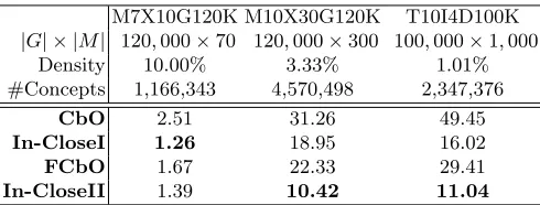
Artificial data sets were used that, although partly randomised, were con-strained by properties of real data sets, such as many valued attributes with a fixed number of possible values. The results of the artificial data set experiments are given in Table 3.
Table 2.Real data set results (timings in seconds).
Mushroom Adult Internet Ads Student
|G| × |M| 8,124×125 32,561×124 3,279×1,565 587×145
Density 17.36% 11.29% 0.97% 24.50%
#Concepts 226,921 1,388,469 16,570 2,276,0243
CbO 0.66 3.06 0.56 32.68
In-CloseI 0.40 1.65 0.12 11.42
FCbO 0.35 2.06 0.21 17.20
In-CloseII 0.29 1.62 0.10 9.38
Table 3.Artificial data set results (timings in seconds).
M7X10G120K M10X30G120K T10I4D100K
|G| × |M| 120,000×70 120,000×300 100,000×1,000
Density 10.00% 3.33% 1.01%
#Concepts 1,166,343 4,570,498 2,347,376
CbO 2.51 31.26 49.45
In-CloseI 1.26 18.95 16.02
FCbO 1.67 22.33 29.41
In-CloseII 1.39 10.42 11.04
8
Conclusions and Further Work
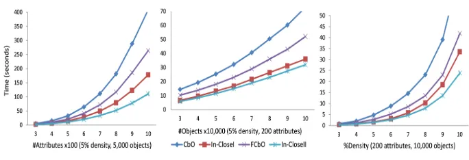
The results of the performance experiments suggest that the partial-closure canonicity test significantly improves the efficiency of CbO-type algorithms. Not only was In-CloseI faster than the basic CbO algorithm, in most cases it was faster than FCbO. Although FCbO can significantly reduce the number of clo-sures carried out [26] this appears to be outweighed by the savings in intersections made by partial-closure.
The results also show that further efficiency is possible by combining ad-vances in CbO: combining the inherited canonicity test failure of FCbO with the partial closure canonicity test of In-CloseI to create In-CloseII. In most cases In-CloseII was faster than In-CloseI, but it is interesting that for the objects series of randomised experiments the saving was relatively small and for the ar-tificial data set M7X10G120K, In-CloseI was actually faster. It is quite possible that the complexity of the inherited failure feature is resulting in some signifi-cant overheads in the computation, but further work is required to confirm and investigate this suspicion. It may be enlightening to compare the effort saved by the reduction of intersection operations with the increased effort of passing, updating and accessing the inherited failed intents.
[image:13.612.185.430.268.361.2]Fig. 3. Comparison of performance with varying number of attributes, density and objects.
Implementations of In-Close and FCbO are available open-source at Source-Forge [4, 27].
References
1. S. Andrews. In-close, a fast algorithm for computing formal concepts. In
S. Rudolph, F. Dau, and S. O. Kuznetsov, editors, ICCS 2009, volume
483 ofCEUR WS.
http://sunsite.informatik.rwth-aachen.de/Publications/CEUR-WS/Vol-483/, 2009.
2. S. Andrews. In-close2, a high performance formal concept miner. In S. Andrews,
S. Polovina, R. Hill, and B. Akhgar, editors,Conceptual Structures for
Discover-ing Knowledge - ProceedDiscover-ings of the 19th International Conference on Conceptual Structures (ICCS), pages 50–62. Springer, 2011.
3. S. Andrews. Appendix to: A partial-closure canonicity test to increase the efficiency of cbo-type algorithms, 2013.
4. S. Andrews. In-close program, 2013.
5. S. Andrews and C. Orphanides. Analysis of large data sets using formal concept lattices. In Kryszkiewicz and Obiedkov [18], pages 104–115.
6. D. Borchman. A generalized next-closure algorithm - enumerating semilattice
elements from a generating set. pages 9–20. Universidad de Malaga, 2012.
7. J. P. Bordat. Calcul pratique du treillis de galois dune correspondance. Math. Sci.
Hum., 96:31–47, 1986.
8. C. Carpineto and G. Romano. Concept Data Analysis: Theory and Applications.
J. Wiley, 2004.
9. M. Chein. Algorithme de recherche des sous-matrices premires dune matrice.Bull.
Math. Soc. Sci. Math. R.S. Roumanie, 13:21–25, 1969.
10. A. Frank and A. Asuncion. UCI machine learning repository:
http://archive.ics.uci.edu/ml, 2010.
11. B. Ganter. Two basic algorithms in concept analysis. FB4-Preprint 831, TH
Darmstadt, 1984.
12. B. Ganter and R. Wille. Formal Concept Analysis: Mathematical Foundations.
13. R. Godin, R. Missaoui, and H Alaoui. Incremental concept formation algorithms
based on galois lattices. Computational Intelligence, 11(2):246–267, 1995.
14. M. Kaytoue, S. Duplessis, S.O. Kuznetsov, and A. Napoli. Two fca-based methods
for mining gene expression data. In S. Ferre and S. Rudolph, editors,ICFCA 2009,
volume 5548 ofLNAI. Springer, 2009.
15. M. Kirchberg, E. Leonardi, Y. S. Tan, S. Link, R. K. L. Ko, and B. S. Lee. Formal
concept discovery in semantic web data. volume 7278 of LNAI. Springer-Verlag
Berlin Heidelberg, 2012.
16. P. Krajca, J. Outrata, and V. Vychodil. Parallel recursive algorithm for fca. In
R. Belohavlek and S.O. Kuznetsov, editors,CLA 2008, 2008.
17. P. Krajca, V. Vychodil, and J. Outrata. Advances in algorithms based on cbo. In Kryszkiewicz and Obiedkov [18], pages 325–337.
18. M. Kryszkiewicz and S. Obiedkov, editors. 7th International Conference on
Con-cept Lattices and Their Applications, CLA 2010, Seville. University of Sevilla, 2010.
19. O. Kuznetsov, S. A fast algorithm for computing all intersections of objects in
a finite semi-lattice. Automatic Documentation and Mathematical Linguistics,
27(5):11–21, 1993.
20. S. O. Kuznetsov. Interpretation on graphs and complexity characteristics of a
search for specific patterns. Automatic Documentation and Mathematical
Linguis-tics, 24(1):37–45, 1989.
21. S.O. Kuznetsov. Learning of simple conceptual graphs from positive and negative
examples. In J.M. Zytkow and J. Rauch, editors,PKDD’99, volume 1704 ofLecture
Notes in Computer Science, pages 384–391. Springer, 1999.
22. S.O. Kuznetsov and S.A. Obiedkov. Comparing performance of algorithms for
generating concept lattices. Journal of Experimental and Theoretical Artificial
Intelligence, 14:189–216, 2002.
23. C. Lindig. Fast concept analysis. InWorking with conceptual structures:
Contri-butions to ICCS 2000, pages 152–161. Aachen: Shaker Verlag, 2000.
24. M. Norris, E. An algorithm for computing the maximal recatangles in a binary
relation.Revue Roumanine de Math´ematiques Pures et Appliqu´ees, 23(2):243–250,
1978.
25. L. Nourine and O. Raynaud. A fast algorithm for building lattices. Information
Procesing Letters, 71:199–204, 1999.
26. Jan Outrata and Vilem Vychodil. Fast algorithm for computing fixpoints of galois
connections induced by object-attribute relational data. Inf. Sci., 185(1):114–127,
February 2012.
27. Krajca P., Outrata J., and Vychodil V. Fcbo program, 2012.
28. F. Strok and A. Neznanov. Comparing and analyzing the computational
complex-ity of fca algorithms. In Proceedings of the 2010 Annual Research Conference of
the South African Institute of Computer Scientists and Information Technologists, pages 417–420, 2010.
29. T. Tanabata, K. Sawase, H. Nobuhara, and B. Bede. Interactive data mining for
image databases based on fca. Journal of Advanced Computational Intelligence
and Intelligent Informatics, 14(3):303–308, 2010.
30. D. Van der Merwe, S.A. Obiedkov, and Kourie D.G. Addintent: A new incremental
algorithm for constructing concept lattices. In P. Eklund, editor, ICFCA 2004,