The partial correlation function in the identification of non linear systems and an eye position transducer

University of Warwick institutional repository: http://go.warwick.ac.uk/wrap A Thesis Submitted for the Degree of PhD at the University of Warwick

http://go.warwick.ac.uk/wrap/74145

This thesis is made available online and is protected by original copyright. Please scroll down to view the document itself.

THE PARTIAL CORRELATION FUNCTION IN THE

IDENTIFICATION OF NON-LINEAR SYSTEMS

and

AN

EYE

POSITION TRANSDUCER.

ToM.W .WEEDON.

This thesis, being a report of research carried

out under the direction of Professor J.L.Douce,

B.Sc., M.Sc., Ph.D., D.Sc., F.I.E.E., C.E., is

subBitted to the University of Warwick for the

degree of Doctor or Philosophy.

Abstract.

Section 1.

A correlation technique is developed which enables the identification of systems belonging to a restricted class of

non-linear systems. The method is applicable to a syst~ which may be

represented as a single-valued, instantaneous, ti~e-invariant

non-linearity followed by linear dynamics. The characteristic of the

non-linearity and the impulse response of the linear element are

found simultaneously in a single eA~eriment.

A class of pseudo-r~ndom test signals is studied, and results are derived for sorne situations in which the results are contaminated

by noise.

Further work is required to extend the applicability of the

·technique, to compare its performance with other methods of

identifi-cation, nnd to investigate alternative test signals.

Section 2.

A simple eye-position transducer is described, which measures

eyeball rotation about two axes.· Dependine upon the characteristics

of the subject's eye, and the operating conditions, an accuracy of as

good as

!

5%

may be obtained over a range of 120.

The user wears a light-weight infra-red optical-electronic

device on a spectacle frame. The transducer exploits the variation

in infra-red reflectivity over the surface of the eyeball, and

therefore varies in its performance from one subject to another.

It may be used by some subjects in all liehting conditions except

. direct sunlight.

Further work is needed to e~lminate the deficiencies of the

device, but an investigation into television techniques, which are

Seotion 3.

The experimental determination of the region of asymptotic

stability of a second order time invariant system may be considerably

simplified by taking advantage of the nature of the trajectories

Yhich form the boundary of the region. These trajectories are found

easily by reverse time simulation.

Further york is possible to investigate the extension of the

Acknowledrnent

I Ba grateful for the continuous help of ~y supervisor

Professor J.L.Douce, and for the support of the Science Research

,·Council. Also for the help and encouragement froTllTlY Tlany friends,

I

including those nentioned below, to all of wh~ I say 'Thank you'.

HR.L .BUD1ER.

MINISTRY OF AVIATION (R.A.E. BEDFORD)

UNIVERSITY OF 1"AR1VICK (ELECTRONICS WORKSHOP) UNIVERSITY OF 'tlAR~VICK (SCIENCE LIBRARIAN) UNIVERSITY OF T.fARWICK

UNIVERSITY OF ~"AR~VICK(SCIENCE LIBRARIAN) HINISTRY OF TECHNOLOGY (N.P.L.)

MINISTRY OF TECHNOLOGY (N.P.L.) UNIVERSITY OF l.fARWICK

HR.B.D.ARMSTRONG. MR.J .L.BAKER.

MR.J.K.CANf'(ELL. . MR.J .DAVIES.

MR.K.R.GODFREY. MR .P .H .HANHOND• DReM.T .G .HUGHES.

MRJ·f .S.HUNT. UNIVERSITY OF WARWICK

MR.R.L.HYDE. BRITISH AIRCRAFT CORPORATION

MR .H .S .P .JONES •

DR.K.C.NG.

UNIVERSITY OF WAR~aCK

UNIVERSITY OF WAmaCK (ENGThTEERING WORKSHOPS)

UNIVERSITY OF ~vARWICK UNIVERSITY OF ~.fAR~lICK MR.A.J.McINTYRE.

MR.P.C.PARKS.

PROF .J .G. THOHASON• I.C.I.

ABSTRACT

LIST OF CONTENTS

INTRODUCTION

SECTION 1. THE PARTIAL CORRELATION FUNCTION in the

identification of non-linear s.ystems.

. . '

Chapter 1. Introduction. 1

"

..

-1.1 I~pulse testing by cross correlation.

•

.Chapter 2. The Partial Correlation Function. 5

6

2.1 Definitions of Partial Correlation Functions.

2.2 The Use of the Partial Correlation Function 10

2.5

in the Identification of Non-linear .Systems.

Quantised Signals.

Periodic Input Signals.

Periodic, Quantised Input Signals.

11

12

14

Chapter 3.

3.1 Realisation.of a Test Signal for

Identification.

The p-1eve1 m-sequence.

15

16

3.3 Identification Using the p-leve1

m-sequence. 21

3.4 The Power Spectr~ of the Output of a

Non-linearity with p-level II-sequenceinput 23

Chapter 4.

Identification in the Presence of Noise

31

4.2 Identification of a System when the Input

Test Signal is Contaminated By Noise

4.3 Identification of a Non-linear SystellWhose

Chapter 5.

References.

Ap~endix 1.

.App()ndix2.

Appendix 3.

Appendix I..

Appendix 5.

Appendix 6.

Appendix

7.

Appendix 8.

Identification Using a p-level m-sequence

~hen the System Output is Contaminated

by Noise.

35

39

1.0

Conclusion.

The Partial Correlation Function of the

Input and Output of a Non-linear System. 1.1

The Cross-correlation Bet~een the

Co~ponents of a p-level m-sequence. 43

1.9

Identification Using a p-level m-sequence.

The Auto correlation Function of the Output

of a Non-linearity with p-level m-sequence

Input. 52

The Power Spectrum of a Signal Having a

Periodic Spikey Autocorrelation Function.

Identification of a Non-Linear System ~hen

Measurements of the Output are Contaminated

by Noise. 59

The Autocorrelation Function of a Clocked

Signal.

62

Identification of a Non-linear System ~hen

the Input Test Signal is Contaminated by

SECTION 2. AN EYE POSITION TRANSDUCER.

Chapter 1.

Chapter 2.

Introduction.

The Design and Development.of a Transducer

Based on the N.P.L. Version of Young's

Instrument.

Design of the Geometry. 2.1

2.2 Modification for Use in Any Lighting

Condi tiona.

Modification for Use in Two Dirtensions.

Practical 'Work.

Observations ",ith the Eye Position

Transducer, and with the Infra-red

Inage Converter.

3.2

Prelininary Experi~ents in Typewriter

Chapter

3.

3.1

Control •.

General Experimental Observations.

Chapter

4.

Conclusion.

References.

Appendix 1. The Common Area of Two Circles.

Appendix 2. Linearity.

SECTION 3. EXPERD1ENTAL DETEm1INATION OF THE REGION

OF ASD1PTOTIC STABILITY BY

REVERSE TIME

snruLA

TIOM •

68

74

77

82

84

8;

8;

87

89

90

92

93

97

i

INTRODUCTION.

This thesis is co~posed of three sections. The first describes

work on the identification of a class of non-linear systems by a

cross-correlation technique. The second describes an instru~ent for

the Beasur~ent of eyeball position. The third consists of a paper

published in 'Electronics Letters' on an experimental method of

dete~ining syste~ stability.

Except where indicated, all of the work was carried out at the

SECTION 1.

I.

Chapter 1.

An engineer designing a controller for a given plant needs to know

the characteristics of the plant, in terms of some relationship between

its input and output, before he can achieve satisfactory performance

from the s.ystem of plant and controller. The more stringent is the

specification for system performance, the more detailed, and the more

accurate

.

_.

must be his knowledge of the plant. By considering the nature of the plant he will be able to construct a theoretical model of the

plant. Depending upon the extent of his initial knowledge, he will

then need to carry out an experimental investigation to determine the

suitability and parameters of his model. This is one example of the

need to 'identify' a system; to find experimentally the relationship

between its input and output.

If the plant is a linear system, it may be characterised by its

frequency response, or by its impulse response. The two characterisations

are equivalent, and each may be found from the other. Also, each may be

related to the theoretical model in terms of a differential equation.

This suggests two possible approaches to the identification of the plant.

The first is to generate a sinusoidal input to the plant and measure the

resulting gain and phase. By carrying out this procedure for all input

frequencies the frequency response of the system is found. The second

is to measure (as a time function) the output in response to an impulse

input.

Unfortunately both methods have severe disadvantages. Sine wave

testing is a very lengthy process, as the plant must be allowed to

settle to a steady state after the application 6f each new frequency.

Impulse testing must be carried out with very low input signal levels

otherwise the plant may be driven outside its region of linear operation.

Frequently economic consideration3dictate that the plant should remain

in service while the identification is performed. This means that the

2.

that the test signal must be kept to a very low level to maintain

satisfactory limits on the plant output. The signal to noise ratio may

be very small therefore, and reasonable results may only be obtained by

averaging over many observations.

Consequently, indirect methods have been developed to find the

impulse response of a linear system. As the time derivative of a unit

step is a unit impulse, for a linear S,ystem, the impulse response is

the time derivative of the step response. Step response testing still

gives a poor signal to noise ratio for the high frequency components.

1.1

3.

Impulse Testing hy Cros~-correlation.

~(t)

Linear System

~(t)

yet)

figure 1.1.1

In chapter (2) we define the cross-correlation function, a

measure of the dependence of one signal upon the past values of

another. ~.Jealso define the auto-correIa ti on function which is a

measure of the dependence of a signal upon its own past value. It

can be shown (see, for example, Douce 1 Chapter (6) ) that the

cross-correlation function of the input and output of a linear system

is the convolution of the auto-correlation function of the input and

. the impulse response of the system. That is, for the system of

figure (1) CD

S:;Xy(r) =

L

W(I> !h:r(T-v)d.v 1.1.1

Where ~v(t) is the system impulse response

~Iy(T) is the cross-correlation function of x(t) and yet) A random signal has an auto-correlation function which is

impulsive, because its current value is independent of all its past

values. ~e can see from equation (1) that if x(t) is a random signal,

then the cross-correlation function of the input and output is the

impulse response of the system.

~y(r)

=

WeT)

when

~X(T)

=

aCT)

We have therefore, an indirect method of finding the impulse

response of the system, summarised in figure (2)

x(t) _{Linear System} yet) _Correlator ~.,(T

wet)

I

)

Random Signal.

The normal operating input of the plant may well be a random

signal, and therefore suitable as the input test signal. As the

auto-correlation function of a short length of a rand~ signal is not

necessarily impulsive, an experiment using the operating input must

be very carefully designed, and the statistics of the input signal

monitored over the time period of the experiment. This may be

,

overcome by introducing a test signal which is deterministic and has

statistics (notably its auto-correlation function) similar to that of

a truly random signal. In section (3.2) we meet a class of deterministic

signals which, in addition to having kno~n statistics over a short sample,

Chapter 2.

In chapter (1) we saw hm~ by correlation we could find the

impulse response of a linear system. In this chapter we will

define the partial correlation function and see how it may be used

(2.1) Definitions of Partial Correlation Functions.

Consider two signals, each a function of time, x(t) and yet)

The cross-correlation function ~y (T) is a measure of the dependence

6,

of the value of y(t+T) upon the value of x(t). It is defined by the

relationship

00 00

~y

(T)

=

J J

X.Y.p(X,Y,T).dX.dY 2.1.1

_co ..00

where p(X,Y,T) is the joint probability density function of

x(t) and y(t+T). That is,

P[X" x(t) < (X +

Sx)]=

p(X,Y,T).SX.SY Y ~ yet) < (Y + SY)

SX, Sy .. o, •

*

We may rewrite equation

(1)

as

co 00

~y (T)

=

J

X [

J

Y.p(X,Y,T) dY

JdX

"00 ..co

Let us now consider the term in curly brackets. This we will call

the partial cross-correlation function, ¢Xy(T,X). Clearly the

partial cross correlation function is a function of the time shift T,

as was

~xy(T),

and is in addition a function of the value of X for which

it is evaluated, as a result of the dependence of p(X,y,T) on X.

We now define the partial cross-correlation function ¢Xy(T,X) of

x(t) and yet) with respect to x(t) as 00

~.v

(T,l)~~I'P(X'Y'T)

dY

and it is clear from the definition that co

!xy

(T)

=

J

X.~xy

(T,X)

dX

---2.1.2

-00

*' The symbol P

I ••• )

is used to mean litheprobability that the

statement in curly brackets is true".

H Equations are numbered starting from 1 in each section, with the

'section number as a prefix. tVithin the section the prefix is omitted.

1-Physically, ~xy(T,X) is the expected value of y at a time T after

x

=

X. It is the function which West2 calls the 'ti~e dependent mean

density function'. If x has a mean value that is zero, then

~Xy(T,X)

becomes Nuttall's g-function~

We will nryJ define a component signal, a(t,X), of x(t) such that

a(t,X).oX

=

1,

x ~

x(t) < X +

oX

oX

-+

0

=

0, other"Jise _2.1.4

X~b'<

X

I II

I I I _t

I , I I I

I,

1/

"by. r :r-

.,

t

r-~ __ ~~u_ __ ~ __ +- ~

c

figure 2.1.1

from this definition we see that co

x(t)

= _[

X. a(t,X).OX

If x(t) is an ergodic process, the probability that x lies between

X and

(X

+

oX)

is

oX.Px (X)

=

limit

₁

t

SX. aCt,X) .dt·

T-+oo 2T _-T

and so _{Px (X)}

₌

_limit

₁

J;

_{a(t,X) dt}

T-+oo 2T

2.1.6

"

where

Px

(X) is the probability density function of x,

P

Ix ~

x < X +

cSxl

=

SX. Px(X)

now,

a(t,Xd. a(t+!,X2). OX2

=

1, [X1 ~ x(t) < X1 +

sx

X2 ~ X(t+T) < Xa + OX

=

0, otherwise

8

so it follows that for an ergodic process

T

Px (X1,X2,T).OX2

=

1i:init:.

.1

!

a(t,Xd.a(t+T,X2) OX~ dt

T .. '0) 2T -T

and

T

=:

lirtit

1

1

a(t,Xd. a(t+T,X2).dt

- T ""0:>2T -T .

where Px (Xl,X2

,T)

is the joint probability density of x(t)

and X(t+T).

Let us now return, from OGr digression on component signals, to the

correlation functions. If x(t) and yet) are ergodic processes, then

we may write their cross-correlation, ~y(T) as

T

thy (T)=:li::1it

11

x(t).y(t+T)dt

, T'" eo 2T -T

2.1.8

and by substituting equation (5) into this expression

, TO).

~y (T)=·l~mit'].

1!

X.a(t,X).y(t+T)dX.dt

T .. 0) 2T -T-co

1

0) T

=

X [lirriit

1J

a(t,x).y(t+T)dtJ dX

_ co T .. co 2T -T

clearly the term in curly brackets is the cross-corrolation ~ay(T)

between a(t,X) and yet) co

~Y(-r:)

=

L

X giaY(T) dX

Comparing equations

(3)

and

(9)

we see that

PXY (T,X)

=

!1iaY(T)

where !1iay(T) is tho cross-correlation function between

a(t,X) and yet)

Hence, if x(t) and yet) are ergodic,

f/>:ty (T,X)=~lb1it'

l1T

a(t,X)y(t+T)dt

, T'':'' Co 2T -T .',

2.1.10

If we now replace y by x in all the previous expressions, we find the

auto-correlation function, !1ixX(T),and partial auto-correlation function,

~XX(T,X),of the signal x(t)

~.c

r)

=

J~J~

x••x••~x.,x.,r) .ex ••

dX.

-00 -00

2.1.11

00

~xx(T,X)

=

!

X1.P(X,X1,T).dX1

- 00

2.1.12

If x(t) is an ergodic process, then

T

~:dT)=~ limit'

1

1

x(t) .X(t+T) .dt

T' ....·w·)2T T

~xx(T,X)=:limit

1/

Ta(t,X).x(t+T).dt

T-" ·00.2T -T

By substituting equation (5) into (13) and (14),

~X(T)

=

/0I:1°°X1.X2. !l5a1a:a(T).dX1.dX:a -00 -00

<i>XX(T,X)=

Joo

X1!15aa1(T)dX1

-00

where ~aa1(T) is the cross-correlation between a(t,X)

and a(t,Xd

9

2.1.13

2.1.14

2.1.15

2.1.16

10.

Ihe Use of the Partial Correlation Function in the Identification

_ W' of Non-Linear Systems.

" The partial correlatton. function may be used in the identification

of Borne non-linear systems. These are the systems which may be

represented by figure

(1),

where a single-valued inst~ntaneous non-linearity, defined for all inputs, is followed by a linear system.

x(t)

~ y ~ f{x)

Ld~~)J

ott)

z(t)

,...

figure 2.2.1

In appendix

(1),

the partial cross-correlation function

¢X~(T,X) of x(t) and z(t) is found to be

0) 0)

<P:r~(T,X)::

J

W(v)! f(X1) ~aa1(T-v).dX1.dv

J,l::o X1=-OQ

where ~aa1(T) is the cross-correlation function of the components a(t,X) and a(t,X1) of the input x(t)

If ~aa1(T)

=

0, for all X~1' and all T

2.2.1

then, ~

"':t~(T,X) =

rtx) /

W(V).~aa (T-v)dv 2.2.2

11=0

where ~aa(T) is the autocorrelation function of'a(t,X) ,' ,::,

if,"further, lZiaaer) .has an i:npulsive form,

then,

2.2.3

In practice there is a signal which has properties closely

approximating those of x(t) above, and which we will discuss in

chapter

(3).

Using this signal and a partial correlation process we can identify the dynamics of the linear system, and find the

II

Q~ntis~d Signals.

'Nhen the input signal x(t) is quanti sed into, say, p levels

(X

O

,X1, ••••XP-1)' the component signal a{t,X) of x(t) must be zero

when X~ XL' one of the p levels.

=

0,

x

=

Xt

=

x(t) )

)

otherwise )

l)X. a(t,X)

=

1,

We see that a(t,X) is a unit impulse,

a(t,X) = 5(X-XL),

=0

x(t)

=

XL

,

otherwi3e

)

, )

)

It will be convenient when x(t) is quanti sed to write

XL+S

aCt,i) =

J

a(t,X).dX

Xt ..

o

where 20 « (Xt- Xt-i)

Xt+S

~xJCr,i)

=

!

~X3(r,X).dX

Xt-S

from equation (2), we see that a(t,X) is always zero outside the limits

used in equations

(3)

and

(4).

We recall that s1>x3(r,X)

=

Joo

Z.p(X,Z,r).dZ

-0:)

which is zero outside the limits used in equations (3) and

(4)

since

p(X,Z,r) =0,

so in place of equations (2.1.5), (2.1.10) and (2.1.3), for a quanti sed

.ignal ~:

x(t)

=

-0 <px,( r,i)

=

Xl. a(t,i)

T

1i'nit

1...!

a(t,i).z(t +r)dt T .. 00 2T

-T

2.3.6

(for x( t).•

~p

ergodic process)

~:I.

T)

=

rx

to i'.,( T.i) 2.3.7

and equation (2;=2~1) becomes .

ifn}.

Toil

=

JM

11(.)

r,

1'(X;). "'iaj (T - .)d. 2.3.8

o J=o

12.

.

Let us consider the partial cross-correlation function of two

ergodic signals x(t) and Z1(t) with respect to aCt). We found in section

j

(2.1) that this may be written

T

CP:t~1(T,X)

=

limit

.L

J

a(t,X).Z1(t + T).dt 2.4.1

~' ~ co 2T .

-T .

where a(t,X) is a component signal of x(t)

It x(t) is periodic, with period Tc, then

(.

x(t + NTc)

=

x(t) for all integer N

Let Z1(t)

=

z(t) + net)

where z(t) is periodic, wi~h period Te, and net) has no component

wi th period Te.

Since Z1(t) is ergodic, and z(t) is ergodic as a periodic signal i~

necessarily so, then net) is ergodic

T

c/>X'J1(T ,X) = limit

_L

J.

a(t,X).z(t + T)dt

T -> co 2T _{-T .}

T C

+ limit

_.L

J

a(t,X).n(t + r)dt

2.4.3

T ~ co 2T

-T

Now the first term in equation (3) is the average over.all time

ot

a(t,X) and z(t +

T).

Since both signals have period Te, they will

maintain the same phase relationship over all time, and so the average

1s the same as the average over one period. T

T C

limit

1

J

a(t,X).z(t + T).dt

=

1

J

a(t,X).z(t + T).dt

T ~ co 2T -T

're

o

As net) has no component "dth period Te, the second term in equation (3)

is just the product of the expected values of a(t,X) and net)

T

limit _1

r

aCt,X) .n(t + r)dt

=

E {a(t,X)}.E {nCt}}

T~O) 2T

LT

Te

8~

J

I

~X~1CTJX)

=

1

a(t,X).z(t + T)dt + E ia(t,x)}. E {net)}

Te

2.4.4

o

A special case is when net) has zero mean value, equation

(4)

then.

beccme e

Tc .

= 1

J

a·(t,X).z(t+ T)dt

In particular, equation (5) holds if net)

=

0, for instance if x(t) and z(t) are the input and output of a noise free system.

If net) has zero mean value, the cross-correlation function

~X31(T)

is given by Tc

~31(T)

=

i

f

x(t).z(t +T)dt

o

2.4.6

It is important to obeerve that it is z(t + T) that appears under the

integral sign in equations

(5)

and

(6),

and not Z1(t +

T).

Errors occur in estimates, of ¢X31(T,X) or of

~X31(T),

based on correlation

performed with Z1 for a finite integration time, since in general

even when E{n(t)}

=

0, Tc

f

x(t).n(t + T).dtl- 0

This isOtaken into account in appendix (6) where the variance of such

an estimate is found.

In chapter

(4)

we will study the identification of the system of figure

(1),

in which the output z(t) is contaminated by noise net).

figure

2.4.1

~e see from equation (5) that if net) has zero mean,

q,X~1( T,X)

=

<PX3 (T,X)

This suggests that we could use an experimental estimate of 9X3~T,X)

14

2.5

,reriodic, Qu~ntised Input Signnls.

•

. !ve will be dealing bter with quanti sed signals which are periodic •

For this case, the results of both sections (2.3) and (2.4) are

applicable, and we will summarize them here in a combined form, for

future use P-l

x(i) _=L X t. a(t,i)

a(t,i) t=o x(t) X t

where

=

1

,

=

2.5.1

=

0, otherwise

x(t)

=

x(t + NTc)

2.5.2

where Tc is the period of x(t) and N is any integer

Tc

ct>X3l(T,i)

= 1

J

a(t,i).z(t + T).dt Tc

o

where z l(t) = z(t) + n(t)

2.5.3

n(t) has z~~ mean, and is uncorrelated with x(t)

~3l( r)

=

X t. cJ>X3l( T,i)

L=o

Also, it is obvious from equation (2) that

a(t,i) = aCt + NTc,i)

If W(II) = 0 for v~ Te, then equation (2.3.8) becomes

Tc

Pf1\

~X3(T,i)

=

J

W(v) ~ fj.·~ataj(T - v)dV

which is the par%ia1 cro~s~corre1ation function of the input and

output of the system in figure (2.2.1), with respect to a quantised,

Chapter

C3l: "

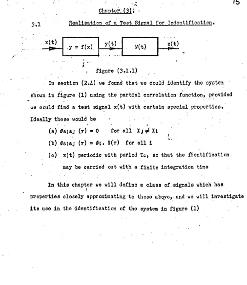
Realisation of a Test Signal for Indentification •

. .~ .7.= rex)

I

y~~ ...1_'_W(_t _)

__'I-I_~

...

(t_) .~

,

~' ~.

;

figure (.:3.1.1)

In section (2.4) ~e found that we could identify the system .

sh'ownin figure (l) using the partial correlation function, .provdded we could find a test signal x(t) with certain special properties.

Ideally these would be

i I

for all IJ ~ Xt

(b) ~alaJ

(T)

=

~L.

SeT)

for all i

(c) x(t) periodic ~ith period Te, so that the £aentification

,

~,

may be c~rried out wit~ a finite integration time

In this chapter we will define a class of signals which has

!

properties closely approximating 'to those abq_~e" and ,we will investigate

[image:25.542.6.512.14.596.2]

Ib

The p - level rn - sequence.

A random number sequence is a sequence of numbers in which each

element is independent of all previous elements. \Je may consider a

particular random signal which is generated from such a random sequence,

,in the follo1~ing way. A generator produces an output which may change

only at the instants when regularly spaced clock pulses are recei~9d by

the generator. The output after the arrival of a clock pulse is independent

of the output before the pulse arrived. Let us find the autocorrelation

function ~rr{T) of the output r(t), when the clock period is A. ~rr(iA)

=

E{r(t).r(t -iA)} for all integer i

= E{r(t)} E{r(t -iA)jfor all i~ 0

=

E2{r (t )} for all i

f:

0

!Z>rr(0)

=

Elr2(t)}

In appendix (7) it is sh~~n that the autocorrelation function

of a clocked signal changes linearly between T

=

i.)" and T

=

(i + 1) A for all i, so we have the correlation function sh~~n in figure (I)

The feature at the time origin is defined in appendix (5) as a 'spike',

~nd approximates to an impulse of strength (E{r2(t)} _ E2{r(t)}}.A

~lr. (tlJ

.:i,\(Tl

BJ1{.tJi

:"---I

L

I

rjr

-x

0 A T

figure (3.2.l)

A pseudo-random sequence is a periodic number sequence which

has 'statistical properties approximating to those of a random number

sequence. In particular, the autocorrelation function of a pseudo-random

sequence is similar to that of the random sequence.

Clearly, as the pseudo-random sequence is periodic, its

auto-correlation function must be periodic and so the best approximation that

could be obtained is shown in figure (2) where Tc is the period of the

I:t-j"

---

'\---

- ----

-

-,

\

"

\

. -. --_.-.. _...

_/

\

__

figure (3.2.2)

I. _

1'0

..~

o

t

In practice it may also have other spikes of various heights

in each period. Of course, if the signal is physically realisable

these spikes cannot be of magnitude greater than the one at the time

origin.

Now consider a register of n stages, each of which has p stable

states. Upon receipt of a (regularly spaced) clock pulse, each stage

adopts the state of the previous stage before the clock pulse. Such a

register is called a p-level n-stage shift register, and is represented

in figure (.'3)

---'. c.leck.

.~..r

·--1---~·-·--·---·~--·-=·-·~-·~

C.-o(""-;l

)C-'_''_!

et

j C2

I .

.--..----.

r

~'tl'-I

t

r---- ---.----.._...

e , •. ~ - .

c,.

shift

figure (3.2.3)

Ot (t) is the state of (and output from) the ith stage at time t.

We may write

dt(t)

=

CL-l (t - A) i

=

1, 2, •••• n

where A is the period between clock pulses.

If the input to the shift register, co(t), is formed by modulo p

operations upon the outputs Cl(t) ••• cn(t), we have a feedback shift

register as represented in figure

(4)

18

!.fe can describe the operation of this device by the equation

Where the symbol

<:....

::>P

is used to mean that the operations

between the b~ackets

<

and> are all performed modulo p,

If p is a prime, we may choose a1, a2 •••••• an such that co(t)

is a periodic sequence of (pn - 1) elements, in the course of which

every n-tuple (C11 C2 •••• cn) occurs once, except the null n-tuple

(0, 0, 0 ••• 0) and this never occurs. Such a sequence is a

'maximal-length pseudo random p-level sequence

t,

and we will refer to it as a

~level m-sequence.

The p-level m-sequence has (p-l) equally spaced spikes in each

period of its autocorrelation function. If the levels Xo, Xi ••• Xp-i

of the output of the shift register are chosen symmetrically about

zero, then the mean value of the sequence is zero and the

auto-correlation function is zero, between the (p-l) spikes in each period.

Some of the spikes may have zero amplitude, for example if (p=4N+l, N

integer) then the spikes at delays of one quarter and three quarters

I

of a period are of zero amplitude.

Figure (5) is an example of the autocorrelation function of a

p-1evel m-sequence. In this case p = 3, so there are jus·1;two spikes

in each period of the autocorre1s.tion function.

fc.:("(,)

IS

-18

Autocorrelation function of a 3-level m-sequence of length

(33 - 1)

=

26] clock periods.

In appendix (2) the cross-correlation functions of the components

of the p-level m-sequence are found. The results are shown in figure

(6) for the general case.

'+--1:

__.1::: _H:i ·t...•••••••»,. .it:

• 1 ~ .

!::: :;;_{1;:: '::'}.. ;;::

·-1"

.,:: ::i: ;,; :::. ';;; ;:::.1.1 '" ••••••••.•••

7TTI

I" ••

"ITT"

,1;-;," :r;;••••

,., .,j ,"1'·' .,.. ,.

·l-:'~i,.·

"i:' . 'I'"

• I ~•

·:··1·:· ::::1:::

::::k

::::1:: .

. ~. ' t··.

:: :n:

••• ,1.

'11' '." .".,' j;;: :::, :::: .. '

r

ItI li!1 f'!!'!"il'l' ,':[:11::: ::;: :::; 'i:: .: , Ht! i;"IHl11 !n:

, mt

ni Ht :';11::: .;;i !::; ; ;: :it :jf! ;. 1 rtt: , ..tt '".

t

!

t lid (II ::11;:1: :::: ::,: :::: :::; :, : ;:P 1:1' t:!l :P:

i ! t ~ 1t:.. ;;:: .::: ::;; :~:: ;~;''! i :It: .:.!r:r: ::;: ., ..

l!;: j:j: _t:

"'1

,1'1 _;11:

:II :,.:n: :_"

.' ,t~,

.: t:':

21

Identification Using the p-level m-sequence.

It is clear from figure (3.2.6) that the p-level m-sequence

does not meet our specification for a test signal. The cross-correlation

between any two components is the sum of a non-zero constant, and a

function yhich has spikes for T

=

o,~,

2 Te etc p-l p-l

However, consider the identification of the system in section (2.2).

For a periodic quantised input signal x{t), and a noise free system,

the input-output partial cross-correlation function ¢xJ(T,i) is given

by equation {2. 5.~ as -1

. <1',.

(T,i)

=

J

C \1(V)! fj

.~'L

OJ(T - v)dv

o j=o

yhere W(I)

=

0, _{IJ ~} Te

~aLaJ{T) is the cross-correlation function of a{t,i)

and a(t,j)

fi

=

f(Xt)

The constant term in ~ataj(T) produces a term CL in ¢x3(T,i) which

is independent of T but dependent on i. Ci depends upon the characteristic

of the non-linearity a~d upon the integral

e

.

J

T,.[{IJ) dll

. 0

and is therefore unknown.

We see that if 1,.1(v)

=

0, for

v ~ ~),

then over the range p-l

o

~T<..I£. , the spikes in ~ataJ(T) which are not at the origin bave p-l

no effect.

Hence, if W{v)

=

0 for v 7 (~) we can use the p-level m-sequence for p-l

identification, but we will have to remove the constant term Ct. We

will see later how to achieve this.

In appendix (3) ye derive an expression for ¢x3{T,i) in terms

of the parameters of the m-sequence, and those of the system, with the

result· n 1 [

¢X3{T,0)

= ~

·(r(o) - fav).~(T)

p -1'

fTC

J

. + (fav -

.ficl)

W(II )dll

pll_l

o

~xJ(r,i)

= ~~

[eft - fav)W(r)

1Xtlo p -1

provided that (1)

W(r)

has a

Tc

+ fay / W(V)dV].

o

(2) W(r)

=

0,

settling time long compared yith A

r

1~~1)~1}

1\

and where fali

=

1:

L

fj

p .

J

If ye were mechanising the identification on a digital computer, we

would compute

¢X3(~'

i) for k

=

O,l, •••m.

where

ni

=

pn - 1

I

-p-l

'hA

and since we have assumed that W(~)

=

0,

~:ra(lv\,O)

=

p~-1[(f(O) - fay·).W(~)

p -1

~:r3(1~,i) = 'p~-1

[(£t -

fav).~"(kA)

+

xtlo

p -1

m

+ (fay - ~Ol) \' 1-1(jA)] P -1 ~

JTI_ J=O

fay

L

W(jA)]

J=o

3.3.5

It is clear that

for all k, i

If we form a matrix of measurements [Mkt] such that

Mkt

=

pn_l

[4>:J:

a(kA,i) - <ha(mA,i)]

pn"'1

then Mkt

=

W(lv\). (fi-fay' 3.3.7

Now we have the same information as we would have had if we

had performed the identification with our ideal test signal, except

that ye are unable to find fay from MtJ.

We are unable to find the equivalent gain ot the non-linearity

either from equation (7) or from equation (2.2.3), but this is

3.4

The Pover Spectrum of the Output of a Non-lineari ty .~ith

..l?=levelm-sequence input.

..

p-level n-stage instantaneous

feedback

shift-xlt) single-valued

y(

t) }or

register _{non-linearity}

clock period I~ y

=

f(x)

figure

3.4.1

Consider the system of figure

(1).

We assume that the

feedback connections to the shift-register have been made such that

x(t) is an m-sequence of period Te,

Te

=

(pn_l)",

In appendix

(4)

we found the autocorrelation functions ~xx(T) and gyy( T) for this case. When p >2, ~y( T) was found for T an integer

~y( T)

=

p~-2[

7jlqT1 P -1 (a) fJ

=

f(XJ)

where

(b) T1

= ~

p-1

(c) q

=

0,1, •••• p-2

(d) B is the delay gain bo which corresponds to T1(see appendix (2) )

We see from equation (2) that when the average value ~ ~ tt of

t=o

the non-linearity is zero, and when it has zero output for zero input,

then there is no constant level in the autocorrelation function of

yet).

Generally this will not be so, and there will be a constant level d in

the autocorrelation function 9yy(T), given by equation (2)

From equatlon

(1)

we see that spikes occur regularly at delays

",Kq, q

=

0,1, •••• having heights Hq (see figure (2), so that

Hq

=

pn-1 [\=~f«Bq Xt)p).ft

-1 (~

ft

)2J

pn_l

L

p

L

2.4-'fhe power spectrum Gllyy(W) of yet) is the sum of an impulse

of strength d at zero frequency, due to the constant component d, and

G'yy(w), the power spectrum of the spikes alone. G'yy(w) was found in

appendix (A. 5)

G"yy{w)

=

d.S(w) + G'yy(w)

where (a) G'yy(w)

=

sinc2

t.h\

.Gyy{w)

Tc

(b)

(c)

0-3

....,.._

Gyy(w)

=[

Ho+(-1)h

Hp;'.

+ 2 ~ Hq.gyy(w,Kq)

J

gyy(w,Kq)

=

1

.Cos 21:"~ q=1

').. Tc

(d) his any integer.

(e) sinc x ~ sin x x

So G'yy(w) is the line spectrum sinc2nh').., where h is

Tc

integral, modulated by a periodic function of h, Gyy{w) which has a

period in h of (p-l). We need evaluate Gyy(w) only for the (p-l) values

h

=

O,1, ••••p-2, to determine it for all values of h.

The complete power spectrum of y, in terms of the parameters of

the system and of the m-sequence is

. GII{W)

=

o{w).[

~[r·1fLJ~_

~J

p -1 ~ p -1

L=o

+

1

p~-1 sinc2

nh')..

\'

[

Cos211hg.

').. p -1 Tc

L

p-l

[r

f(BqXtl p) .ft -

i/~

fI)']]

L=o L=o

where h is an integer.

25

where the symbols have the same meanings as in equation (2).

By the same method that we used to find G"yy (w), we find that

Gq.,(w)

=.1 •

p~-1 sinc' llhA )~ :[ Cos 21Th9

t.. P -1 Tc p-1

2:<BQ.X,)p.

,x'J=O

3.4.7 and once again we ha~eoa modulated sinc2 function.

An Example

A five 'level m-sequence is generated by a two stage shift

register which has B

=

2 and clock period one second. This sequence is

the input to a saturation ~on-1inearity y

=

f(x), given below. i.e. p

=

5, n

=

2, B

=

2, 'A.

=

1

x -2 -1 0 1 2

y, -1 -1 0 1 1

A!J

-l -I /

~-I'

2

For T, ~he delay, a whole number of clock periods, the

autocorrelation function of the m-sequence is

)

n-1[

2-~

q

J

~:c:x:(qT1

= ~

<B.X L) s.x L

P -1 __J .

"=1

~x( ~Ts)

=

0

. p~-1

=

j_

p -1 24

q

=

0,

1 }

=

4 + 1 + 1 + 4

=

10 q

=

1,3, { ]

= -

2 + 2 + 2 - 2

=

0

•

q

=

2, {

J

=

-10

and the autocorrelation function of the m-sequence is the full

·~.,_.;TJ_'i':al~('-c)

26

.'\"_' f:t{'<::)

~---~~-~

figure

3.4.3

For T an integer number of clock periods, !Pyy (Tfrs)

=

0, sinoe fo

=

0, and ~: fl

=

°

~y ('1.T~ = ~-1

[{'~«BQ

.XJ)p) .fJ

r:

fo2

p -1

L

J

pn_1

r=

n-1 I:;

~

=

""'-p -1 24

q

=

0, {

}=

+ 1 + 1 + 1+ 1

=

4

q = 1,

3,1

}= - 1 + 1 +~ ~ 1 = 0

q = 2,

1

}= - 1 - 1 - 1 - 1 = - 4

and the autocorrelation function of the output yet) of the

non-linearity is the dotted line in figure

(3).

We may now find the functions Gxx(w) and Gyy(w) using equation (5b)

G:x:x(w)

=

i.

x 101 1 - (-If

I

=

100 , h odd

24. 24

=

0 ,h even

Gyy{w) =i.x4{1- (-If}

24

= 112

,h odd 24

=

0 ,h even

,So the power spectrum of x(t) is the function sinc2 m1 (see figure

24

(4)

modulated by Gx:x:(w)(see figure (5). The power spectrum of yet) is the same sinc2 function, modulated by the function Gyy(w) (see figure

(6).

For this particular non-linearity, the autocorrelation function

,.1·

• t~ •

.1...••_,.

...

:1;:

!-i:.:

.1 ••

; rr :

.... ::;;

.... ., .

: :~••••••• H

.: f>v.t-c- :~: '"

:: :.:.;:. :;6'q.-+:-!:-::...:;_.:~~~

::::0:

...

: ~ ; • : t : I,. ...

.... ,l .. ,11,

I... .

,••. ~ •..;".•';... .;..''-I'....;..; C';.t.i

~~ii ... +•• ~1 ~ ;

••••• 1.

I ...1.·.

I-.~-'~'-'.~'-:-;~-.-f-::-~1--1:f-i-i

i-

;:+-.;~-~-q._:-.~'-.;-f-;i-;-H._~-~r;..·;+-,~...;l-~';...1{,-;~~~: ;I

T:

+m

~'~;1';"::+-~:;..;~~'-:+--;:.:;.;..;i:..J:':';;';~':';+--::'::-::J,' -: ;';ij:':i1.;:':::.:.:~:~!.:.;_;.;:;;_.+.:_;.':'.:.J, c:.'l.:;_'+;.;::~c:.;;.;;;L:~':";;;_'+...::' ~.:.~.:..·IL:t.;..;;:_;::~ ;;~

I~~

t :;:;

i~:

,1- .

._

,.

• • ~ •1 ••

~i~!~~!::d~i:l~

~~i:r:':~ii~

nn

;:.::p:::::~E:

....:~~l~~~~r~~:

:.:;.!1-::: :!;:

:~~....

..._ _.~ _,.-

-

._. .... .

:~:~ : 1:'

... .-....

... -... • ....~.-+ ••

·tr: ::.,: ._...• ::..::.

-.

"'-+t· ...

"4 ..•..

., ,.

..

~

.

'H'

::~~A:-:i:

::~;f;;~()::'i:~~:~~:bf~_;::::r::d::;~~::':::::;:;.:r:.JD:+::~:t~:

.- ....}iU~~;::::!:::ir; :.::;~~;:i~: :;~~:::~'I'~T

'~E::::3t;;:4~4::

::cY"

:::':1••.

:=s..::

::::-!~::

:ii~t:-s

j~ ~:~;:::t:.::

::.:: ::-:: ::;: :-.t::: :.~::1:-:-7

Hz.rrr: :::: it;; ~ ;~...•.. -=+--t

tt:: :.!:: ... :::r _,

:;: ...

'1'1 ., ••

.

,...

*f¥.~:

....

t:::

.n:

:r:: ....,

....

..,. :1 ~ ., " " ::;; .~.: :1:; ::;: :r:' r:::

.1,· ::1:_:1::

'1.'....

. :1:

..,.

..

28

Another Example

We will take the m-sequence of the previous example as the

input to a modulus non-linearity, given belO\l.

x -2 -1 0 1 2

Y 2 1 0 1 2

J

t~

2

,/

-, _/

+ t-'

-1 -I 2.

The autocorrelation function of the non-linearity output is

_P-1

g5yy (T

F

Ts) = pn-2 [\- 'fL

J2

= ~

pn_l

L

.

2

L=o

(since fo

=

0)

~y (qT1)

=

f~[

~«B"

.Xj>

j>fJ

J

~ - j_

p -1 24

q = 0, { }=

4

+ 1 + 1 +

4

= 10

q

=

1,3,

1=

2 + 2 + 2 + 2

=

8

q

=

2,

{1

=

4

+ 1 +

1

+

4

=

10

The autocorrelation function of yet) is the dotted line in

figure (7). The autocorrelation function of the m-sequence is

reproduced as the full line in figure (7), for comparison.

50

2+ _{\ "" /\ . '" / '_"-}jj{Y)}

\... - - _'" ..._ - - _I \ '" , -.I \

The power spectrum Gyy(w) is given by equation (5b)

h

Gyy(w) =

1- {

14(1 + (-1) ) +

B

Cos

~l

~ 2

=

2,

h =

0,4,B, ••••

2

= 0, h = 1,5,9,••••

=

j, h

=

2,6,10, •••• 6

=

0, h

=

3,7,11, ••••

Gllyy(W) = ~ 8(w) + sinc2-17'h • Gyy(w)

2 24

Gyy(w) is plotted in figure (9) with Gxx(w) in figure

(B)

;;;: ~ ;;;:·t-~~~-··~·-·~I·-·~ ... :~::I;':: :;:: •.+-~. • ~... ...

~!:::i: :

'"1"-.' _. ~_.,.• '-t.. ~ ...

..._

...+,

,._....

-l::: ... _..,.._. ....:;.;_....

-

~ ..

.... ::~~ t.':':: ., ..

...1 .

... _o.

:T::: .

....- I'"

... -t '

~:.:

"

....,,.

._

·~··~·.j.:·';'''~·F+~';';::~:',::: ..

.... ,_... t·, .•.. h' ',;: ::1 : :::1 ·.t· .~.:I~. • ....t ... >-, •.

.••. ·to

..-0-•••••••••••

:;::I~::b!:

::..·I~.::V.

..-. ·tt· _.

... ~ .

4- ... ~ I'" - ••

... , .

~:;: f!.i~:~:-1'

~.: _{. .:-t ..._}'.' ..•. '·0' ..•_I.,·

... ~..

..._{...- ~} . - .

, , .

:-:--:~ :-:. :!::

,..

..

,. ".,...: ~! :.._,. ··t·

....

..

,. .,..

....

::1: ..._:~~:-t!::,'

••-t.

·t'·

.,..

••• - M"

.;:: ::-;-; ... 1. ',' '" ...

.

. ::u

g~ ,.. .".1.· .

::::

" "";;::

:;; .... .r.: ::!: ...:::; .d, .••• :.'••i.: .... :.t':.:..•.. :.j'~.:.• ~... :t.· •.:.: !;;. ,::: :::: ;~:t .," .•r .• :ii; ;;ii ;.'f.i:.· ~:!!....:':"1':. :.~r,: ;.••.:.:.... -.:t!:i::: ..

·:1..···

::-::1:::

:::~ ~::~:~:~·~"~·~~~·~·~"~~~.;.;t'~~~4~"~'~'~';';f~~~~:·ri·i~:~~··'.~·~;~~~~~~~.~.~..~~~:+.~.i~:i~.~..~~14~·'~·~·~';';f~~~~~~l~~~~.t-·~"~·~·~·~·.+-··t··· ::I. . .. t... .•.. :t·I·.•·:'.'1: :a: ,.,. ... ..~;·H· :;~; ~.l.'.:;. ::;: ~t;.; ., .. ~f~' ;;ij i','i; :1:: .~•. ::~~:!:: .... .... .::....:;.Ij::

rl~ :::: :;;: "" ::1: 'j.. ... '1' ~:il ::-1: :t:: ~r:, :~i! 'r:: :::: T;:: :::t d~: "" 'r:: .. oIH .t-*. .... . ...

"I,

::!: ...._{:::: .}"·f"·_"... ,., .:!!:'" ...,.. :.:t:

::;:

:tl:

.ti:

....

>-1"

... ·t··

...

::;: ;j." ;Jp ,...

...

.·t-.~

..

.:~.i:

;<h::

;~i:i~:·

::::

::!: ." :::: :!:!

..

,

1'-',.

:1::

:.r: ::!:

..."-_..

. --:t:-:-:

...-_.

....,...

;;:: I:C:

~i:~:~::~:~.f;·_··;,;·~:I..;.;_:r:~:~:I+-:t;..:~'r:~:.·::+-'';';'-1'.:::

tl ~:::: .... ..t· qf ~ toI. ., T • • • • •••

..

"

'1,·

:;;:

.".

.,.

I I ~

.,.

.... 1

..~, ::-!! "".1,1

.-1" ;;:;

.1 ••

31

Cha.pter 4.

4.1

Identification in the nresence of noise.

. In any experimental situation, the various signals within

a system viII be contaminated by noise, due to disturbances to the

,system. Also, any measurements will be contaminated by noise, due in

part to the instruments. Let us consider the effect of this on t.he

system of figure

(1)

which we have been studying.

_h Non- linear

Linearity. system

- ..., ".

. .

figure

4.1.1

The non-linearity is likely to be an element in which noise

'\..

injection can only take place at its input or output, a non-linear

transducer for example. lYhen this is the case we may represent the

non-linearity in the noisy environment as in figure (2)

non-linearity

n2,(t)

1--'-~~~_""--;iI;'-'

figure

4.1.2

The linear part of the system is more likely to be a distributed

dynamic system with noise injection taking place at various points. As

it is a linear system, the output will be the sum of the outputs dUd to

each of the inputs (the signal input and the noise in~uts), individually •.

We can therefore represent the linear system in the noisy environment by

figure

(3)

W (--r)

+

I

net)

IP

;®-*-figure

4.1.3

.The noise net) in figure (3) can take account of all noise sources

at the input to the linear system and all noise sources in the measurement

of the output. We may consider the entire system as in figure

(4)

non-linearity

linear system

32

4.2 Identification of a non-linen.r system ,,,henthe input .

test signal is contaminated by noise.

y

=f(x+n)

ly(t~1

'N(r) z(t)

For the sake of completeness, this situation is investigated

in appendix

(8).

If (a) the signal to noise po~er ratio is high

(b) x(t) and n(t) are uncorrelated

(c) n(t) has zero mean

then the estimate rX3 (r,X) of 9X3 (r ,X) is unbiassed,

where _Tc

=

1

J

a(t,X).z(t + r)dt

Tc o

The variance of this estimate is found in appendix (8), but

the result does not give any insight into the situation, and is

33

4.3

Identification of a non-linear system whose output is contaminated by noise.

1

n(t)

y

=

rex)

I

yet)

L-.I_W_(_V_)

-ojl

.(t)

Cb "

(t) x(t)

figure

4•

.3.1

Consider the system of figure

(1).

This represents the non-linear system which we have considered, and takes account of

any noise injection after the output of the non linearity, as we

saw in section

(4.1)

We make an estimate r :J:3(T,X) of the partial cross-correlation

function ¢X3(T,X), by integrating over one period of the input signal,

to give Te

rX3(T,X)

=1

j

a(t,X).Z1(t + T)dt Te

o

where a(t,X) is a component of x(t), as defined in section 2.1

In appendix (6) we find that rX3(T,X) is an unbiassed estimate

of ~X3(T,X) if the effective noise input net) at the system output

(a) is ergodic

(b) has zero mean value

(0) is uncorrelated with x(t)

In the same appendix the variance, a2 of the estimate is shown

to be

Te

(]2 =

Z

j(T

e -II).q;nn(v). q5a~II).dlJ

Tc2

o

whe~e

~nn(V)

and

q5~a(V)

are the autocorrelation functions of

net) and of a(t,X) respectively.

Clearly a

2

is independent of

T,

and

Qnn(V)

is independent of X.

When x(t) is an m-sequence, ~aa(V) is independent of X for all X

F

0, and

the variance of our estimate is independent of X and T. In many cases,

the variance for X

=

0 is similar to that for X

F

0, but this depends upon the autocorrelation function of the noise, and must be checked in

An Example.

Let us consider the identification of the system in figure (1)

when x(t) is a p-level m-sequence, and net) has the auto-correlation

function shown in figure (2)

-A

'"

o

'~

figure 4.3.2

net) could be, for example, a random clocked signal or an m-sequence

with period longer than that of x(t). In particular it could be a

binary m-sequence, which would be useful in a simulation to test the

theory that has been developed so far, because of its ease of generation.

We will assume that x(t) and net) are uncorrelated.

Let us take the very simple case An=A, the clock period of the

m-sequence generator producing x(t)

=

0

,

otherwise

applying equation

(2),

and inserting the results for a p-level

m-sequence we have, for X

F

0,

0'2

=

Z

.C. p~-2

!

(Tc - II). (1 -~) (p - (p - 1) J! )dll

T~ (p 1-1) .).. )..

o

=

C • p;;-2 [ 4pn+1 + 2p n - ~ -3J .4.3.3

(; (p _1)3 _

for X

=

0, ..._.. (,

A

0'2

=

Z •

C. pn-2

!(

Tc - II). (1 - J!) (p - (p - 1)L ) dII

T~ (pn_l) }.. }..

o A

- Z

.C. _L_

!

(Tc - II). (1 -

.u.J

dll

T~ (pn_l) )..

o

=

Q • _L_ [pn-2(4 n+a + 2pn - 5p - 3) - (6p" - S>] 4.3.4

6 (pn_l)3

We see that· the variance for X

=

0 (equation

(4),

is a small amount

35

4.4

Identification usine A p=level m-sequence ·.Jhenthe

System Output is Contaminated by Noise.

y

=

f(xl

IY(~l

I

~(tl

x(t)

".

In section

(3.3)

we considered identification with an m-sequence, In section (4.3) we considered the 'general effects of noise at the

system output. So far we have not asked the question 'Given experimental

estimates of the partial correlation function, what are f(x) and T,{(t)?'.

It is the purpose of this section to ansver the question, given the

following

assumptions:-(1)

net) is stationary and not correlated to x(t)

(2) The autocorrelation function of net) is such that the

variance in estimates of the partial correlation function

is independent of the level X for which the function is found.

(It is in any case the same for all non-zero X, but may differ

for X

=

0, see equation 4.3.2.)

We saw in section

(3.3)

(Equation

(3.3.6»

that

~~l

[9X3 (jA,Xtl - ¢X3(mA,XIl]

=

flowJ

where A is the clock period of the m-sequence,

Wj

=

W(JA)

,..

ft

=

f(Xt) - ray

fav

= ~

r

f(XI)

L=o WJ

=

0, j >,.. m

Let us define a matrix of measurements _{,._}M, where

M

=

[111J]

-11tJ

=

[r:z:

J(j A ,i) - ~ :x: J(rnA,i )

J

.If.=l

pn-.l

36,

From our previous work, and assumption (2),

"

Ht J

=

ft. Wj + E'Lj .

where the matrix of errors [E't J] has elements etj independent of t and j. ~

~'le '..Jish to choose ft and ~'Tj to be the best fit to the data H in the se~5a that the variance, C, ls minimized where

C =

L

Ld~j

:3 t j ,.,.

- (M' .

r.

H.)2

E'tJ - . ~J - L· I"IJ __

ac

=:

-22_t

Lj .'Jj +

2LA

.r,.[j2

=

0 for Cmax or min

oh

j j

~.

=

-2\Etj

.ft

+ 2)fL2 .T.Tj

=

0 for C max or min

a""

••J

/..:.;

L t

Rewriting these last two equations in matrix terms,

a

C

=

2 (

t

.~;r

.!,[ - NW)

=

0

a¥'

- - -

_-ac

=

2(}!.tri -

NTf}

=

0

0\'1 ...

-

A

where

~f

,}! and I are

ac

=

W

-Wj oC

at;

= oC

'it;:

= I oC

art

_..

equations (5) and (6) yield

}1

H

=

I

HT

:l

-

MTr = ~.,

iT

'f

,-..J-

---for which,

M }1T~ =a2

of

~A..,I-

-where

....,

We would like to know how many solutions £or·a2 are oommon to

equations (9) and

(10).

This is dependent on the ranks of the matrices

llMT and NTH.

Let us assume that H is an mxn matrix_..., and that mcn ,

..

(In the rest of this section, we will use m,n and r as parameters of the matrices,

and not in their former roles). The other case (that m>n) yields a

similar result by the same method. Generally ...!e would expect the

rank r of M to be m, but the follO'Jing is quite general and admits

'-'

the possi bili ty that r<rn.

l1NT is an m x m matrix, and MTH is an n x n matrix. The number

__ _-.J

of non-zero eigen values in equation (9) is the rank of W1T, and the

_'oJ

number of non-zero eigen values in equation (10) is the rank of HTl.f •

.

--In text books of matrix algebra it is shown that

(1)

the rank of a matrix is unchanged by elementary row operations. (2) the rank of a matrix is unchanged by elementary column

opera ti ons ,

(3) any number of elementary row operations may be represented by

premultiplication by a non-singular matrix.

(4)

any number of elementary colUMn operations may be represented

,

by post multiplication by a non-singular matrix.

So, if M has rank r' there

- ~IRIB]

P H

=

'V, ...,

"V,

_,-

06;-06 ~

00

is a matrix P such that

"'-J

where ~ is an r x r non-singular matrix.

_4.4.12

hence

!

=

,.:.-1

['!!~~J

000

.,

~l!T

=

!~

[~~!]

000

. I'.J

R 0

A 0

...

r [;:]

,/\ where :.,

= ~

~T + ~;:T + ~

13~-r

'It

~~~

38,

J!:,!,Tis ':":vedefinite, ~!..T and ~ are +ve semi definite, so.£. is non

singular. C is an r x r subnat.rd,x, hence H HT is of rank r ,

,.-....~ ..." -..,..

A similar use of elementary column operations shows that 11TH is

-~

--'

also of rank r.

There are r non-zero eigen values of equation (9) and r non-zero

eigen values of equation (la); we must now find h ov many eigen values

are common to bcth ,

Let us assume that ~ is an eigen vector of equation (9) and a2

is a corresponding eigen value.

i \! MT ,... - ",,2 ...

• e.

--

'"

....

co -" co prernultiplying by HT,

_...

11TM HT ~

=

(J2 HT ~

....,.. ~ ~."I ..,_,

clearly, by canparison of this with equation (io),

_-

ET.:;is an eigen

vector of equation (la), and ~ is the corresponding eigen value.

We see that all of the: r non-zero eigen values of equation (9)

are eigen values of equation

(10),

and so all the non-zero eigen vectors are common to both.

To minimise the computation required, we should find the'eigen vectors

and eigen values of whichever of equations (9) and (la) has the ~aller

order. If m <n , then ~,fMT is m x in and smaller then ~~TU. So the

I"'tJ ,._, 'W ,_,

,..

estimation of

r

and ~ becomes

(1)

find eigenvector and eigenvalue of equation

(9)

to obtain ...

"

a2 and

f

"

premultiply

!

by.~ to obtain ~

"

"

scale f and/or ~ such that

IfI2.1~12

=

a2 •

(2)

(:3)

1\ .

Unfortunately this will give us r sets of (%2 , f and J:!.eachone

corresponding to a local minimum in the variance.S (see equation (4"'.).

'.

,-We must therefore evaluate C for each set to obtain the true minlmum~'

"-"

Remembering that the eigenvalues are related to the sizes of the

vectors ~ and

f

by equation

(11),

we see that the eigenvectors

corresponding to zero eigenvalues are for this case null-vectors, and

Experimental work was carried out vd.th an anaLogue aimu.la-tion of the non - linear system, and also with a digital simulation of the system. The former was unsatisfactory because of a period of ~~\Ulreliabili ty of the analogue computer. The digital simulation

'39

Conclusion

Chanter 5.

The technique which has been developed in the preceeding

chapters allows the characteristics of certain non-linear

time-invariant systems to be found in a single experiment. The method

is restricted to those systems which may be represented as a

non-linear elenent followed by linear dynamics. The non-linear element must be instantaneous and single-valued. The characteristic of the

non-linearity and the impulse response of the dyn~ics are found

simultaneously.

Further work is required on the partial-correlation function,

and on its application to identification, particularly in the presence

of noise. The following notes suronarise the work that is required.

1. An investigation of the application of the method to an

extended class of non-linear syst~s.

2. A comparison of the partial correlation technique with other

methods of identification, in the presence of noise. For

instance, the rela.tive efficiencies of this method and

repetitive experiments with binary signals could be found

for various noisey environments. This would be helpful in

determining the value of the partial correlation functions

in identification.

~

Preliminary experiments suggest that the identification of

non-linear systems by the partial correlation technique is

readily implemented by digital computer. Further work is

required to establish pro gran requirements, and to compare

them with those of other methods.

4.

The feasability of finding alternative test signals should

be investigated.

~ Please see note opposite •

40

'References.

I}. Douce, J .L., An Introduction to the Hathematics of

Servomechanisms, E.U.P., 1963.

2}.

3}.

1.Jest, J

.C.,

Non-linear Signal Distortion Correlation. I"tU't\Q.t.:r.co>'l.t,o(Cc;.s)J "01.2,rlo.b, 52.9 -3S (f9bS)

Vuttall, A.H., Theory and Application of tha Separable Class of Random Processes, H.l.T.Technical Report No.343.,

l~ay 1958.

4).

Zierler, N., Linear Recurring Sequences,

J. Soc. Indust. Appl. Uaths. Vol. 7, No.1, p.31•

5). Dickson, L.E., Modern Elementary Theory of Numbers,

University of Chicago Press, 1939.

, 6}. Neuton, G.C., GO:lld, L ••'., Y.,"!.iA'3:', J.F., The Analytical

Appendix (1)

+1

ThA Partial Correlation function of the innut

____...and output of El. non-linear system.

x(t) . y

=

f(x) yet) Wet) z(t)

[N] [L]

figure A.l.l

Consider the system of figure (1). An instantaneous

non-linearity [N]has an output yet) related to its input x(t) by the

equation yet)

=

f(x(t» A.I.l

'~ere f(X) is single-valued (i.e. to each value of x there

corresponds one, and only one, va.Iue of y).

The output of the non-linearity is applied to the input of a

linear dynamic element [L], having an impulse response wet).

Let us now investigate the result of forming the partial

cross-correlation function of the input x(t) and the output z(t), with·

I

respect to the input. The parti~l cross-correlation function ¢XJ(T,X)

was defined for two ergodic signals x(t) and z(t) in section (2.1).

It was expressed (equation 2.1.6) in terms of the component signal

a(t,X) of x(t) as

T

¢X3(T,X)

=

limit _l

f

a(t,X).z(t + T).dt

T .. co 2T

-T

A.I.2

where

co

x(t)

=

f

X.1i(t,X).dX A.1.3

-co

Since [L] is linear, we may express the output z(t) in terms of

the input yet) and the impulse response wet) by the convolution integral, co

z{t)

=

[coW{II). y(t_- 1I).dll A.1.4

where v is a dummy time variable. By equatjons (I) and

(3),

yet)

=

fcof{X). a{t,X).dX A.1.5

42

since by our definition of

[N] ,

the output y of

[N]

for an input X

is rtx)

Frol!l(4) and (5)

.Ct)

=

L~\I

Cv)

ir=-

v,X).dX.dv

So from (2) and (6)

¢X3(T,X) = limit

.L

;r

a(t,X).

L~

(II)

T -..00 2T

LT

A .1.6

00

J

f(X1). a( t + 'T - V,X1 ),dX1.dll.dt A.l.7

-00

Changing the order of integration we get,

¢X3(T,X) =[ooW(II)100f(X1) [ limit

.L

f

a(t,X).

-00 T ...co 2T

LT

·a(t + 'T - II,Xd.dt

J

dX1.dll

r.r.s

Now, we saw in section

(2.1)

that the term in curly brackets is the cross-correlation function, ~aa1(T), of a (t,X) and a(t,X1), and that it is also the joint probability density function Px (X,X1,T - II), so

00 00

¢X3(r,X) =

J

W(II)

!

f(Xd.1SaadT - v).dX1.dll

-00 -co

A.l.9

or

00 co

<P:r3(T,X) =! !V(II)

!

f(X1). Px (X,X1,',r - 1I).dX1.dll

._0) -..00

A.l.lO

Equations (9) and (10) give us a relationship be tveen the partial

cross-correlation function, the characteristics of the system wet) and

43

Appendix (2)

The Cross-correlation bebleen the components

of 8 p-level m-sequence •

.AII the re3ults obtained in this appendix may be found in

Zierler's paper'4.·'. An alternative, more physical approach is

presented here, as Zierler's paper is not easy to read, and the

results are important to this thesis.

,Consider the m-sequence c(t) generated by a p-level n-stage shift register having feedback gains (ai' a2' •• an), and clock

period 1unit. p is a prime. c(t) may take any integer value in the

range 0 ~ c(t) ~ p-l, or in the range - Pil

s

c(t) ~ ~l or any

other range for vhdch modulo pari thmetic has been defined. The work of this appendix is applicable to all of these cases.

c.,IcK.l

t

figure A.2.l

If wa define a dalay operator D, by the relation

nkCc(t»)= cCt - k)

then we may write the following equation to describe the behaviour

of the feedback shift register.

c (t)

=

<

(a nDn + an- 1 nn-1 + ••• a,_D)cCt)

>

p A.2.l where the symbol

< ....

>

p is ueed to mean that the operations

b.etween the brackets

<

and> are carried out modulo p.

Any delayed version c(t -

T),

of cCt) where

T

is an integral number of clock periods may be formed by linear modulo p operations

upon the outputs of the shift register. That is,

c C(t - ~) = (Cbn-1 Dn-i + •••••• +bo)c(t»p

for all T , where N is the number of elements in the sequence, n

N

=

P -·1