Image data compression based on a multiresolution signal model

warwick.ac.uk/lib-publications

A Thesis Submitted for the Degree of PhD at the University of Warwick

Permanent WRAP URL:

http://wrap.warwick.ac.uk/100937

Copyright and reuse:

This thesis is made available online and is protected by original copyright.

Please scroll down to view the document itself.

Please refer to the repository record for this item for information to help you to cite it.

Our policy information is available from the repository home page.

T H E B R I T I S H L I B R A R Y D O C U M E N T SUPPLY CENTR E

TITLE

Image Data Compression

Based On a Multiresolution Signal Model

A U T H O R

IN S T IT U T IO N

and DATE

Attention is drawn t o the fact that the copyright of this thesis rests with its author.

This copy of the thesis has been supplied on condition that anyone w h o consults it is understood to recognise that its copyright rests w ith its author and that no information derived fro m it may be published w ithout the author’s prior w ritte n consent.

T H E B R I T I S H L IB R A R Y

D O C U M E N T SU PPLY C ENTRE

“ n

r

r i - r y n

_____ 1_____ 1 United Kingdom R E D U C T IO N X

Image Data Compression

Based On a Multiresolution Signal Model

Martin Peter Todd B.Sc.

A thesis submitted to The University of Warwick

for the degree of Doctor of Philosophy

Based On a M ultiresolution Signal Model

Martin Peter Todd B.Sc.

A thesis submitted to The University o f Warwick

for the degree of Doctor of Philosophy

November 1989

Summary

Image data compression is an important topic within the general field of image processing. It has practical applications varying from medical imagery to video telephones, and provides significant implications for image modelling theory. In this thesis a new class of linear signal models, linear interpolative multireso­ lution models, is presented and applied to the data compression of a range of natural images. The key property o f these models is that whilst they are non- causal in the two spatial dimensions they are causal in a third dimension, the scale dimension. This leads to computationally efficient predictors which form the basis of the data compression algorithms. Models of varying complexity are presented, ranging from a simple stationary form to one which models visually important features such as lines and edges in terms of scale and orientation. In addition to theoretical results such as related rate distortion functions, the results of applying the compression algorithms to a variety of images are presented. These results compare favourably, particularly at high compression ratios, with many of the techniques described in the literature, both in terms of mean squared quantisation noise and more meaningfully, in terms of perceived visual quality. In particular the use of local orientation over various scales within the consistent spatial interpolative framework of the model significantly reduces perceptually important distortions such as the blocking artefacts often seen with high compression coders. A new algorithm for fast computation of the orientation information required by the adaptive coder is presented which results in an overall computational complexity for the coder which is broadly comparable to that of the simpler non-adaptive coder. This thesis is concluded with a discussion of some of the important issues raised by the work.

Key Words

This work was supported by UK SERC and British Telecom Research Labs

(BTRL), and conducted within the Image and Signal Processing Research

Group in the Department of Computer Science at Warwick University.

I should like to thank all the staff at both the Computer Science Department and

BTRL. In particular, thanks go to all the researchers in the Image and Signal

Processing Group, Abhir Bhalerao, Andrew Calway, Simon Clippingdale,

Roddy McColl and Edward Pearson, for their day to day advice and flow of

ideas.

I should also like to thank my supervisor at BTRL, Dr. Charles Nightingale for

his ideas and support.

Finally I am indebted to my supervisor. Dr. Roland Wilson, without whose gui­

Chapter 1. - INTRODUCTION... 1

1.1 - A General Communications System Model ... ... 2

1.2 - Image Structure, Information and Fidelity... 7

1.3 - A Review of Image Data Compression Techniques ...__...__ 16 1.4 - Thesis Outline ... ... 18

Chapter 2. - LINEAR SIGNAL M O D ELS________________________ 20 2.1 - Introduction ... 20

2.2 - One Dimensional Linear Signal Models... ... ... 23

2.3 - Two Dimensional Linear Multiresolution Signal M odels... 26

2.3.1 - General Linear Multiresolution M odel... ... ... 26

2.3.2 - Quadtree Models... 29

2.3.3 - Laplacian Pyramid M odels____________________________ 32 2.4 - Linear Interpolative Multiresolution Models ... 33

2.4.1 - General Structure______________ _____________________ 33 2.4.2 - Summary of Homogeneous LIM Model Properties... 40

2.5 - Recursive Binary Nesting LIM M odel________ ____________ 42

Chapter 3. - MULTIRESOLUTION PREDICTIVE C O D IN G _________ 52

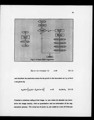
3.1.2 - Prediction Errors and Noiseless C oding... ... 55

3.1.3 - Quantisation ______ __ —__ _______ ________________ _ 59 3.1.4 - Termination or Scale Selection__ _... 61

3.2 - Entropy Coding ... ...I ... 62

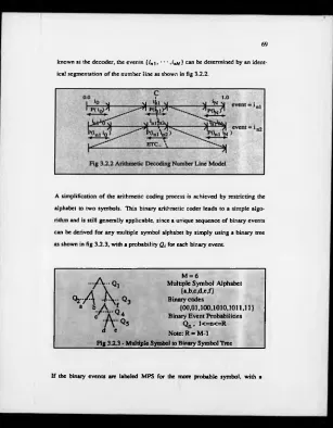
3.2.1 - Arithmetic Coding ... 63

3.2.2 - Adaptive Estimation of the Probability Distribution ... 71

3.2.2 - Arithmetic Coding Results ... ... ... ... ... 73

3.3 - Vector Quantisation____ _____ __ _______________________ 75 3.3.1 - Introduction ... ... 75

3.3.2 - Missing Pixels... ... 78

3.3.3 - Rotation and Reflection Symmetries ... 80

3.3.4 - Vector Quantisation Results___________________________ 82

3.4 - Isotropic Coder Results ..___________ ....______________ ____ 82

Chapter 4. - ADAPTIVE LIM RBN MODELS_____________________ 86

4.1 - Introduction__ ..._____ ________ ____ _____ ________________ 86

4.2 - Inhomogeneous Isotropic LIM RBN M o d el________________ 87

4.2.1 - Scale Selection ______ ____ __________________________ 87

4.2.2 - Summary of Inhomogeneous LIM RBN

Model Properties__ ____ ___________________ ____ 88

4.3 - Multiresolution Isotropic Gauss Markov Models -____...______ 91

4.6 - An Inhomogeneous Anisotropic LIM RBN M odel... 104

4.7 - An Inhomogeneous Anisotropic Colour LIM RBN M odel_______________________________ 105 4.8 - Multiresolution Anisotropic Gauss Markov Models--- --- 108

4.9 - Low-Pass High-Pass Classification ... 113

Chapter 5 . -ANISOTROPIC MULTIRESOLUTION CODING--- 121

5.1 - Orientation M easure________ ________________ _—--- 121

5.2 - Full Orientation Estimator... ... ... ... ... 122

5.3 - Fast Orientation Estim ator... ... ... 124

5.4 - Orientation Consistency... ... 129

5.5 - Prefiltering... ... ... ... ... ... 132

5.6 - Oriented Interpolation--- 138

5.7 - Boundary Pixels--- 140

5.8 - A Homogeneous Anisotropic Codec... 142

5.9 - An Inhomogeneous Anisotropic Codec --- 143

5.10 - An Inhomogeneous Anisotropic Colour Codec _____________ 150 5.11- Comparison of R esults__________________ _____________ 153 Chapter 6. - CONCLUSIONS AND FURTHER W O R K ______________ 155 6.1 - Thesis Summary — --- ...--- ...--- 155

6.2 - Conclusions_________ ______________________ ____ ______ 156

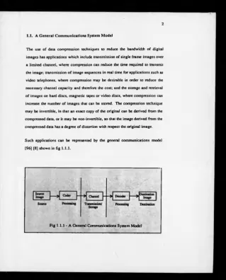
Fig 1.1.1 - A General Communications System Model--- 2

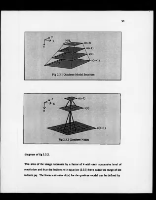
Fig 2.3.1 - Quadtree Model Structure... .— ...— 30

Fig 2.3.2 - Quadtree N odes______________________________________ 30 Fig 2.4.1 - LIM Model Structure ...— --- ... 34

Fig 2.4.2 - Periodicity and Locality Properties of LIM M odel... 41

Fig 2.4.3 - Inhomogeneous LIM Model ...--- --- ---- —... 42

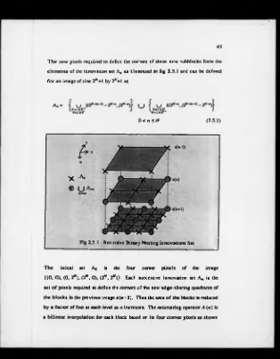
Fig 2.5.1 - Recursive Binary Nesting Innovations S e t... 43

Fig 2.5.2 - Bilinear Block Interpolation ...— 45

Fig 3.1.1 - RBN Hierarchical Segmentation--- 52

Fig 3.1.2 - Bilinear Block Interpolation... ... —... 53

Fig 3.1.3 - New Comer Pixels — .. 53

Fig 3.1.4- Shared Edge Pixels___________________________________ 54 Fig 3.1.5 - Recursive Processing of Blocks in RBN... 55

Fig 3.1.6 - Basic RBN Algorithm...„ ... ... 56

Fig 3.1.7- Peano RBN S can_____________________________________ 57 Fig 3.1.8 - Peano RBN Scan Recursion...— ...--- 57

Fig 3.2.1 - Arithmetic Coding Number Line Model--- 67

Fig 3.2.4 - Binary Arithmetic Coder M odel... ... 70

Fig 3.2.5 - Binary Arithmetic CODEC... ... ... ... 70

Fig 3.3.1 - RBN 5 Point Vector__________________________________ 76 Fig 3.3.2 - 8 Symmetries of 5 Point RBN Vector ... 80

Fig 4.2.1 - Inhomogeneous Innovations B asis--- ....— 88

Fig 4.3.1 - Gauss Markov Model Structure--- --- --- 92

Fig 4.5.1 - Oriented Interpolation... ... ... 101

Fig 4.5.2 - Boundary Innovation Sets--- 102

Fig 4.8.1 - Anisotropic Separable Gauss Markov B lock... 108

Fig 5.3.1 - Fast Estimator Basis P ixels... ... ... 125

Fig 5.5.1 - Brush Stroke Artefacts--- --- --- 132

Fig 5.5.2 - Three Classes of Prefilter... — ...— ... 135

Fig 5.6.1 - Oriented Block Interpolation ... ... ... ... ... ... 139

Fig 5.7.1 - One Dimensional R B N .... ... .... ... 141

Photo 1.1 - Original GIRL Image_____ — ... —— ---— ... 8

Photo 1.2 - Original BOATS Image ... 8

Photo 1.3 - Original LAKE Image --- --- ---— .... 8

Photo 1.4 - Original MISS Image — ... ... ... ... 9

Photo 1.5 - Original TREV Image ___ ____—--- .... 10

Photo 1.6 - Original SPLIT Image --- --- 10

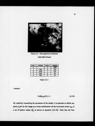
Photo 2.1- Homogeneous Isotropic LIM RBN Model — —...— ... 47

Photo 3.1 - Homogeneous Isotropic RBN Result (GIRL) — --- --- — .— 83

Photo 3.2 - Homogeneous Isotropic RBN Result (BOATS) ... 83

Photo 3.3 - Inhomogeneous Isotropic RBN Result (GIRL)--- 85

Photo 5.2 - Anisotropie RBN Result at 0.32 bpp (G IR L )... —

---Photo 5.3 - Anisotropie Prefiltering (GIRL)... ...»...—...

Photo 5.4 - Sample Anisotropie Filters (G IR L)--- ---

---Photo 5.5 - 0.10 BPP, 28.67 PSNR (GIRL)_________________________

Photo 5.6 - 0.14 BPP, 26.81 PSNR (BOATS)_______________________

Photo 5.7 - 0.25 BPP, 23.66 PSNR (LAKE)_________________________

Photo 5.8 - 0.25 BPP, 30.99 PSNR (GIRL)__________________________

Photo 5.9 - 0.44 BPP, 29.20 PSNR (BOATS)________________________

Photo 5.10 - 0.82 BPP, 25.68 PSNR (LAKE)________________________

Photo 5.11 - 0.08 BPP, 28.14 PSNR (GIRL)________________________

Photo 5.12 - Block Segmentation at 0.08 bpp (G IR L

)---Photo 5.13 - Coding Error at 0.08 bpp (GIRL)... -... ...

Photo 5.14 - Inhomogeneous Anisotropie RBN Result

(MISS)---Photo 5.15 - Inhomogeneous Anisotropie RBN Result (TREV)...

Photo 5.16 - Inhomogeneous Anisotropie RBN Result (SPLIT)... 133 136 136 146 146 146 147 147 147 148 148 148 151 152 152

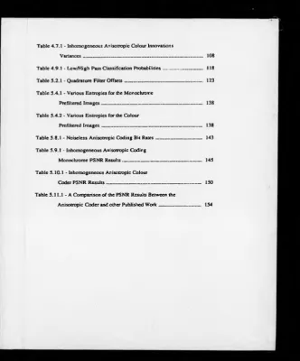
Table 1.2.1 - Various Entropies for the Monochrome Originals --- 12

Table 1.2.2 - Various Entropies for the Colour Originals--- 12

Table 2.5.1 - Estimated Innovations Variances for the

Homogeneous Isotiopic LIM RBN Model (GIRL)--- 47

Table 3.1.1 - RBN Innovations Entropy Calculated

Across all Levels ...---...—...— ... 58

Table 3.1.2 - RBN Innovations Entropy Calculated

for each L ev el...— ...__ —... 59

Table 3.1.3 - Isotropic Noiseless RBN Bit Rates--- 59

Table 3.2.1 - Arithmetic Coding Compression Ratios for

Homogeneous Isotropic Coding Result (GIRL) ...—.... 74

Table 3.2.2 - Arithmetic Coding Compression Ratios for

Inhomogeneous Isotropic Coding Result (GIRL) __... 74

Table 3.4.1 - Homogeneous Isotropic Coding PSNR Results--- 83

Table 3.4.2 - A Comparison of the PSNR Results Between the

Isotropic Coder and other Published W o rk ... ... 84

Table 4.3.1 - Block Splitting Probabilities (GIRL)___________________ 97

Table 4.5.1 - Homogeneous Anisotropic Innovations Variances _________ 103

Variances ...— ... 108

Table 4.9.1 - Low/High Pass Classification Probabilities--- 118

Table 5.2.1 - Quadrature Filter Offsets ... ... ... 123

Table 5.4.1 - Various Entropies for the Monochrome

Prefiltered Im ages... ... ... ...— --- 138

Table 5.4.2 - Various Entropies for the Colour

Prefiltered Images ....--- --- 138

Table 5.8.1 - Noiseless Anisotropic Coding Bit Rates--- 143

Table 5.9.1 - Inhomogeneous Anisotropic Coding

Monochrome PS NR Results--- --- --- 145

Table 5.10.1 - Inhomogeneous Anisotropic Colour

Coder PSNR Results___________________________________ 150

Table 5.11.1 - A Comparison of the PSNR Results Between the

Graph 2.5.1 - RBN Correlation Structure along

j

Graph 2.5.2 - RBN Correlation Structure along

£ J J

Graph 2.5.3 - RBN Correlation Structure along £ j

J

Graph 4.3.1 - Isotropic Multiresolution Gauss-Markov

R(D) M odel____________________________________________ 98

Graph 4.8.1 - Anisotropic Multiresolution Gauss-Markov

R(D) M odel__________________________________________ 112

Graph 4.9.1 - Anisotropic Low/High Pass Gauss-Markov

R(D) M odel___________________________________________ 118

Graph 4.9.2 - Three Different R(D) Models_________________________ 119

Graph 4.9.3 - Three Different R(D) Models (no overheads)... ... 120

logical AND

logical OR

f l iff r = J Kronecker delta function i.e. 8rs =■< q cjsc

CARDM

The cardinality of a set.

HW

The expected value of a random variable.

VARW

The variance of a random variable.

f«l

The ceiling of a, i.e. the minimum integer £ a, for a ^ 0

□

1. Introduction

The increasing use of digital rather than analogue signal representations for sig­

nal processing, and in particular for image processing, is derived from the trac-

tability of many digital techniques which would be impracticable if not impossi­

ble to perform in an analogue form. The techniques opened up by digital image

representations cover a broad spectrum of applications. In image analysis the

aim is to derive significant parameters describing the content and structure o f an

image or sequence of images with a view to object detection, recognition and

classification. In image enhancement, the aim is to make the image more acces­

sible to an observer (either human or machine) by techniques such as image res­

toration, where distortions of the image are to be reduced, or pseudo-colour,

where the structure of the image is made more visible to a human observer for

applications such as medical or satellite imaging.

An additional advantage of digital representation in communication is the abil­

ity to distinguish reliably between information and noise. This leads to greatly

enhanced signal quality for long distance or inherently noisy communication

channels, often without requiring any extra bandwidth to be made available.

Indeed, where the digital representation makes otherwise impractical compres­

sion techniques available, there may be a reduction in bandwidth, or

equivalently of the storage capacity, required for image data. It is the purpose

o f this thesis to describe the development of some new methods for accomplish­

1.1. A General Communications System Model

The use of data compression techniques to reduce the bandwidth of digital

images has applications which include transmission of single frame images over

a limited channel, where compression can reduce the time required to transmit

the image; transmission o f image sequences in real time for applications such as

video telephones, where compression may be desirable in order to reduce the

necessary channel capacity and therefore the cost; and the storage and retrieval

of images on hard discs, magnetic tapes or video discs, where compression can

increase the number of images that can be stored. The compression technique

may be invertible, in that an exact copy of the original can be derived from the

compressed data, or it may be non-invertible, so that the image derived from the

compressed data has a degree of distortion with respect the original image.

Such applications can be represented by the general communications model

[96] [8] shown in fig 1.1.1.

The model consists of five separate components,

(1) Image Source

The source image is a digital signal representation of an image or sequence

o f images which is produced by some well defined source process. Since

this work only considers single frame images, the source is treated as a

process which produces a single image for transmission.

In this thesis, it is assumed that the process produces a source image which

is a regular cartesian lattice of picture elements or pixels with each pixel

position relating directly to a spatial position in the image and that each

such pixel has associated with it a discrete data value (or discrete data vec­

tor) representing the image intensity (or colour) at the appropriate spatial

position in the image.

An important part of the image compression problem is to devise a statisti­

cal model which describes the source images in an adequate manner. The

properties of this source model should be closely related to those of the

image source [51]. From this model various significant parameters of an

image or class of images can be derived, as well as optimal or sub-optimal

techniques for processing such images.

(2) Channel

The function of the channel is to store or transmit the formatted data from

the coder. The channel has a particular capacity, which is a measure of the

amount of information h can handle. The aim of the coder/decoder pair is

to ensure that the rate of the image data is less than or equal to this

o r it may be specified by the systems designer. In general, however, an

increase in channel capacity is usually associated with an increase in sys­

tem cost.

The physical nature of the channel may be anything from an electrical or

optical cable, a telecommunications network, a satellite system, to a mag­

netic tape or disc. Sources of noise will be present in all physical chan­

nels, introducing distortions into the data in transmission across the chan­

nel.

(3) Destination

The purpose of the whole system is to construct at the destination an image

which is an adequate copy of the source image. The criteria for adequacy

will depend on the application and some fidelity measure is devised to

determine the quality of the result. The work in this thesis assumes that

the application involves the destination image being viewed by a human

observer and therefore the fidelity measure should reflect this. However as

discussed in secdon 1.2, all too often the fidelity measure is simply

assumed to be mean squared error. The fidelity measure should be used in

the derivation of optimal or sub-optimal coding techniques.

(4)(5) Coder/Decoder (codec)

The fundamental task of the coder is to transform the source image data

into the form best suited for transmission across the channel and of the

decoder to ‘invert’ this received data back into a form which is as close as

possible to that of the original image data. Berger [8] splits this funda­

"Problem 1: What information should be transmitted ?"

"Problem 2: How should it be transmitted ?"

The first problem is the source coding problem: find the most efficient way to

represent important information from the source; the second problem is channel

coding: protect it against the effects of errors introduced into the received data

by channel noise. The significance of these distortions will depend on the cod­

ing technique (and therefore the source model) and the distortion measure.

In [8] it is shown that, in principle, channel coding can be treated as a separate

issue. Unfortunately, realisable systems cannot afford the unlimited resources

required for this result to hold, particularly if only a single image is to be

transmitted.

Thus in practice the optimal channel coding should be derived with respect to

the source model and fidelity measure in conjunction with source coding. This

is often not considered in the design of compression systems however, either

because the channel characteristics are not known or because the channel is

assumed to be a general purpose channel, with its own error protection coding.

In particular, it is assumed in this thesis that the channel can be regarded as hav­

ing virtually no noise, so that it introduces minimal distortions into the source

coded data. A good example o f this is the case where image data are stored on

the disc of a general purpose computer system, where the computer system has

the responsibility of ensuring the data are not distorted.

While there are applications for which this is not a reasonable assumption, the

work in this thesis is intended to address the issues of source coding and not

those o f the channel coding.

The source coding techniques used may be invertible, in which case the max­

imum compression achievable will be limited by the redundancy in the source

image, or it may be non-invertible, in which case a larger compression will be

achievable at a cost of some degradation of the source image. The source coder

should be directly related to, or derived from, the source model. Indeed it is

sometimes possible to derive an optimal source coder with respect to the source

model and a given fidelity criterion.

Taken together the coder and decoder represent the source coding process and

are referred to as a codec. The design o f a codec is derived explicitly or impli­

citly from a particular source model and fidelity measure. The overall perfor­

mance o f this codec will depend on a good choice o f the source model and

fidelity measure. If the source image has significantly different properties from

the source model, or the fidelity criterion for the application is significandy dif­

ferent from the fidelity measure, then the performance of the derived compres­

sion technique may be poor. The properties of image sources and fidelity cri­

teria are discussed further in section 1.2. Note that although it is sometimes

possible to derive an optimal codec it is not always practical to implement it -

often the optimal codec will require either excessive memory or excessive com­

putation, and a sub-optimal codec must be used.

The source model and fidelity measure can be used to derive a function which

expresses the maximum compression which can be achieved for a given amount

of distortion. This function, formulated by Shannon in 1959 [97] is known as

the Rate Distortion Function and its properties are thoroughly investigated in

the book by Berger [8]. The function is formulated in terms of the statistical

The work in this thesis is aimed at considering some of the issues involved in

image modelling, fidelity measures and derived compression techniques, in par­

ticular with respect to the importance of scale and local orientation as properties

of natural source images. A source model for images with the two properties

mentioned is developed, as well as simple sub-optimal coders for the model and

approximations to the rate distortion functions for related models. In the

remainder o f this chapter some of the basic properties of the source images are

considered, along with some fundamentals of information theory and fidelity

measures, before going on to a brief review of previous work in the area.

1.2. Image Structure, Information and Fidelity

As mentioned in the previous section the work in this thesis assumes the digital

representation to be a regular cartesian lattice of N by M pixels. This is not the only possible representation, but is the most common. In this work, for exam­

ple, images having either N = M = 5 \2 or N = M — 256 are used.

Each pixel in the lattice has a value, or set of values, which represent the

characteristics of the image at that pixel. For a monochrome image the value is

simply a discrete variable representing the quantised light intensity at that pixel.

In this thesis the intensities are assumed to be quantised into 256 equidistant

levels, therefore requiring 8 bits for a simple binary representation. Again this

is not the only possible representation but is the most common. Photos 1.1-1.3

show three original 512 by 512 by 8 bit monochrome images: GIRL, BOATS

and LAKE used as typical examples in this work.

For colour images each pixel has a set of three discrete variables representing

is often used. It is known as the YUV representation [85] [71] and consists of a

Luminance component, Y, and two Chromaticity components, U and V, with each being stored as 8 bits. However, the U and V components are often sub-

sampled by a factor of two with respect to the Y component i.e.

N y = N y= - j N y , and M y= M y — yMy- The colour example images used in this work have N y = M y = N y = M y = N y = M y = 256 with 8 bits per pixel per plane, giving 24 bits per pixel. However the originals came from a source

which had been subsampled in the U and V planes, and therefore a more realis­

tic value is 8 + y + y = 12 bits per pixel. Photos 1.4-1.6 show the original

colour images: MISS, TREV and SPLIT and their respective Y, U and V

planes.

Photo 1.4 - Original MISS Image

Noiseless data compression is possible for such images because o f the inherent

structure within the images and the correlation between local pixel values which

■

---* >

Photo 1.5 - Original TREV Image

M

Photo 1.6 - Original SPLIT Image

redundancy within the data and the total number of bits required to represent the

image can be reduced by techniques which reduce this redundancy. In this sec­

tion a number of simple measures are defined which give the minimum number

of bits required to represent exactly a particular set of image data. Each meas­

ure depends on a particular model o f the image data and clearly the better the

model the better the measure.

The simplest is the zeroth order entropy E° function formulated by Shannon in 1948 [96], which assumes that the data is a sequence of independent data values

taken from an alphabet of possible values {/}, with a given probability distribu­

tion [P (/)}. It is defined as

where L is the size of the alphabet - the number of distinct symbols.

However the data values are often not independent, and the first order entropy

E 1 is a measure which reflects this by relating the occurrence of a given data value to the previous value

where P (i I j ) is the probability that the symbol / will occur given that the sym­ bol j has just occurred.

A alternative measure to E l is the differential entropy E ° which acts not on the data symbols but the differences between successive data symbols. Assuming

that the data symbols represent equally spaced integer values, and by perform­

ing the differences modulo L (with complete invertibility), the alphabet of these differences is of size L, and representing these symbols by e, and their probabil­ ity distribution by P (e), the zeroth order differential entropy is given by

bits per pixel (bpp) (1.2.1)

y - i *-i

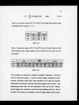
E 0 = - £ P (e) log2 i P (e)] (bpp)

t = \

L

(1.2.3)

Table 1.2.1 gives the values of E°, E 1 and £ ° for the three monochrome origi­

nal images shown in photos 1.1-1.3.

Im a g e G IR L L A K E B O A T S

E° 7 .2 5 7 .6 4 7 .0 7

E l 4 .6 5 5 .5 5 4 .8 0

E° 4 .9 2 5 .9 9 5 .0 6

Table 1.2.1

Table 1.2.2 gives the values of E°, E 1 and E ° for the Y, U and V planes of the three example colour images, together with the sum (T) of the values over the

three planes.

E”m p y

Image

MISS TR EV SPLIT

T

£ " 6.00 5.61 4.67 16.28 6.55 7.16 16.72

£ ‘ 3.90 2.20 2.22 8.32 4.43 1.81 2.19 8.43 4.39 2.02 2.04 8.45 Ed 4.30 2.44 2.28 9.02 4.67 1.91 2.28 8.86 4.72 2.26 2.26 9 .2 4

Table 1.2.2

These entropies are derived for noiseless (invertible) compression, where the

data are represented exactly. In order to achieve higher compression ratios,

however, techniques which allow some distortion of the data are required.

Furthermore, the statistical structure which they express is o f low order - only

neighbouring pixels enter into the expressions (1.2.2), and (1.2.3). Clearly,

natural images have correlations over much longer distances than this. One o f

such long range structure.

The fidelity measure used to assess the degree of distortion in the image should

accurately reflect the application of the compression system. Where the appli­

cation involves a human observer at the destination the fidelity measures should

reflect the human processes of quality assessment. Obviously, the measure can­

not be expected to be an exact model of the entire human visual system, both

because of the complexity of the latter, and since the processes of vision are still

far from understood. However certain properties of the human visual system

are known [69] [38] and these could be incorporated into such a measure [91]

[100]. These properties include edge masking [77], where the presence of an

edge makes noise less visible, and spatial frequency and local orientation selec­

tivity [11] [44] [45] [46] [76].

The work described in this thesis does not attempt to define or use such a meas­

ure explicitly, but the models developed in chapter 4 share certain properties

with the visual system. In particular they reflect the importance of local orien­

tation (anisotropy) and this, together with the spatially inteipolative nature of

the model, leads to derived codecs which produce results with good visual qual­

ity. However, for quantitative comparison with other work (and for the rate dis­

tortion work) the fidelity measure that is used is mean squared error. If s (x,y) are the pixel intensities of the original image and S(x,y) the pixel intensities of the resulting decoded image then the mean squared error is defined as

This measure is often quoted in the literature for image data compression in the

form of the peak signal to noise ratio (PSNR) which is defined as

where P is the peak or maximum value the signal can have. For this thesis, as in most applications, this value is 255, the maximum intensity possible for the

8-bit representation used.

Despite the fact that it is the most common measure used in the literature, it is

not a particularly good choice of fidelity measure with respect to applications

involving a human observer. Take for example the case where each intensity

value in an image is increased by a value of 10. This corresponds to brighten­

ing the image slightly, however virtually no distortion will be apparent to an

observer. Yet the PSNR will be 10 x lo g io -^ - = 28 dB, implying some not

insignificant drop in quality.

A more subtle comparison is given in [56] where two images made up of an

equal amount of white noise are filtered. One is filtered with the filters aligned

at 90 degrees to the local feature orientation of an original image, and the other

at 0 degrees to these orientations. The result is a considerable difference in the

perception of the image (and therefore the quality of the image) even though

they both have the same degree of noise.

It is clear that mean squared error could not be used to represent either of these

significant properties o f perceived quality, but it is still the most commonly

used measure. There are three main reasons for this preference. The first is its

mathematical familiarity. Since mean squared error has been used in many

fields of mathematics, it is well known and many of its properties within other

models have been thoroughly investigated. Secondly it is often mathematically

tractable, so that many problems formulated with respect to mean squared error

have relatively simple solutions. Finally, there is no specific obvious alternative

which would be universally accepted. Although it is possible to derive alterna­

tives based on known properties of the visual system such as frequency

weighted mean squared error [68], the lack of an adequate model for vision

prevents a definitive choice of the best measure, since it would change as

models improve. Therefore, in order to provide some form of universally com­

parable distortion measure, mean squared error and PSNR are usually quoted

for coding results and a more accurate judgement of quality is made by a visual

inspection of the resulting images. This is clearly not a particularly good solu­

tion to the problem, since it assumes that such results can be adequately repro­

duced in publications, which is often not the case. Thus, although the results in

this work quote PSNR’s and the rate distortion functions are with respect to

mean squared error, the photographic prints o f the results give a better indica­

tion o f the success or otherwise of the work.

Finally, the practical codecs described in this thesis have been implemented in

the "C" programming language on a SUN 4/180 running UNIXt. The codecs

were split into separate coder and decoder entities, with the source coded data

from the coder being stored in an intermediary file. All the bit rates quoted in

this thesis (as opposed to entropies) were calculated by taking the physical size

of this file and dividing by the number o f image pixels. The decoder

t UNIX is a trademark o f AT&T Bell Laboratories.

reconstructed the image from the coded source data in the intermediary file. All

the peak signal to noise ratios and mean squared errors quoted in this thesis

were calculated between the original image and this reconstructed image. Thus

the codec results presented represent an upper bound on the rate it is possible to

achieve with these codecs, i.e. they can perform at least as well as the results

presented.

The photographic results were taken on a Dunn Instruments MultiColor unit,

using Kodak TMAX 100 ASA film on the green channel, with an exposure time

of 2.36 seconds, for the monochrome results and Kodak GOLD 100 ASA film,

with exposure times of Red: 2.85 seconds, Green: 2.36 seconds and Blue: 0.83

seconds, for the colour images.

1.3. A Review of Image Data Compression Techniques

This section is intended to be a brief review of relevant work in the area. For a

full review of data compression techniques, the papers by Netravali and Limb

[77], Jain [50] and Kunt, Ikonomopoulos and Kocher [61] and books by Hall

[41] and Clarke [19] provide comprehensive coverage of the area.

The basic framework of the codecs described in this thesis is predictive in

nature, a technique which has been extensively investigated since the early

work o f Oliver [80] and Elias [30]. More recently it has been combined with a

number of techniques such as edge masking [111] [15], multiresolution [110]

and arithmetic coding [4] [36] [73] [74] to provide codecs which are generally

efficient and fairly simple to implement The main drawback o f predictive cod­

ing, however, has been that it is essentially causal, whereas the image signals

are non-causal: there is no preferred direction in an image, unlike a one

dimensional signal.

Transform codecs take a non-causal approach, approximating the eigenvector

transform of the image autocorrelation function [51] and, partly because of this

non-causal nature, generally achieve higher compression ratios than predictive

techniques, but usually at the expense of greater complexity. Two dimensional

transform coders for images were introduced by Andrews and Pratt [5] and a

large volume of work has been published on these techniques [115] [84] [90]

[17] [18] [68], including the book by Clarke [19]. Recent work, such as that of

Chen and Pratt [17], has been based on threshold techniques and there have

been several combinations of transform codecs with other techniques such as

the vector quantiser o f Ho and Gersho [43] and Nasrabadi and King [54], the

pyramid transforms of Wang and Goldberg [108], and selective codecs which

choose between predictive and transform techniques according to their perfor­

mance locally within the image [111].

The significance of the properties of scale within images has been recognised by

the use of multiresolution or pyramid techniques [72]. These have been incor­

porated into other coding techniques such as the predictive quadtree codecs of

Wilson [110] [111] and the transform codecs of Nasrabadi and King [54] and

Wang and Goldberg [108]. Recursive Binary Nesting, which is the predictive

multiresolution framework of the codecs described in this thesis, has been

investigated by Tricker et al [107] and Cordell [24] [25] [26] as well as previ­

ously published work by the author [104] [105] [106]. Multiresolution coding

is related to the subband coding techniques o f Burt and Adelson [2], Woods and

O ’Neil [118], Smith and Barnwell [98], Westerink et al [109] and Kronander

[60], where a signal is separated into a sequence of frequency bands and each

Vector quantisation techniques, which can be formulated as an optimal solution

to the coding problem, have been studied by a number of people [35] [33] [34],

and various adaptive forms have been formulated [54]. However as mentioned

in section 1.2 these optimal codecs are often impractical and so sub-optimal

codecs are devised [86] [103] [42] [12] [55].

There are a number of algorithms which exploit the work on the orientation sen­

sitivity o f the human visual system by Hubei and Wiesel [44] and others [11]

[76], including the work of Ikonomopoulos and Kunt [49] and Wilson, Knuts-

son and Granlund [112].

Other work in the area includes the sketch based coding of Carlsson [16], region

based techniques [59] [71], the representation o f images by higher order poly­

nomials [29] [95], and the so-called ‘model-based’ methods [28] [32] for res­

tricted applications such as ‘head and shoulder’ video-telephone images.

1.4. Thesis Outline

In chapter 2, a homogeneous multiresolution model, the Linear Interpolative

Multiresolution (LIM) model, is formulated for images. It is developed into a

particular form, the LIM RBN model, which is related to the Recursive Binary

Nesting algorithm developed at BTRL [107] for use in single frame image data

compression.

In chapter 3 various RBN codecs are derived for the LIM RBN model of

chapter 2, and their performance is discussed. The implementation of the

necessary segmentation, prediction, quantisation and entropy coding is

In chapter 4 adaptive models are devised to represent the scale selectivity of the

codecs of chapter 3, and the model is then expanded to include the significant

property of local orientation (anisotropy). Several rate distortion functions are

presented for related multiresolution models.

In chapter 5 the techniques needed to implement codecs based on the models of

chapter 4 are described, including orientation estimation, a ‘single consistent

orientation’ measure, anisotropic prefiltering, boundary coding, and oriented

interpolation. The performance of these codecs is discussed.

Conclusions and possibilities for further research are discussed in the final

2. Linear Signal Models

2.1. Introduction

In section 1.1 the importance of deriving the codec from an appropriate source

model was noted. In this chapter some of the issues involved in modelling the

source for natural images are considered and a homogeneous multiresolution

linear signal model for such images is developed. The properties and limita­

tions of this homogeneous model are considered and a specific form of the

model, the Recursive Binary Nesting Model is defined.

As a result of the growing importance of applications for digital images since

the 1960’s, there has been interest in attempts to model the source images both

in order to enhance various image processing techniques and provide a general

theoretical background within which their advantages and limitations can be

considered.

Many of the early models were one dimensional, either as a consequence of

being derived from work on one dimensional signals such as speech, or based

on the raster line scan which is an integral part of most practical image capture

and display systems. These models force the essentially two dimensional

source images into a one dimensional signal, and although the models have had

a degree of success they lack the facility to take account of many of the proper­

ties inherent in the two dimensional nature of images. In the field of data

compression, one set of techniques which have used one dimensional models

extensively are Differential Pulse Code Modulation (DPCM) predictive codecs

The causal linear predictive models which are associated with such codecs take

the form of a predictor and an innovator and essentially exploit the correlation

between successive data values. The predictor seeks to predict the value of a

given data point from the values o f a set of neighbouring data points, and the

innovator provides a correction or innovation to this prediction. If the form of

the predictor is chosen so as to minimise the variance of the innovation terms

then it is known as the minimum variance predictor [50]. For such a predictor

the innovation terms are uncorrelated with the data values, a property which is

desirable in data compression since it also minimises the entropy of the innova­

tion terms [50]. If the data are assumed to be Gaussian, then the minimum vari­

ance predictor is simply a linear combination of the set of neighbouring data

points, hence the name Linear Signal Model.

In order to apply a one dimensional model such as the causal linear predictive

model to an image, a path or time scan must be defined which traverses the

image in a one dimensional manner. The most common scan is the raster scan,

because of its use in capture and display equipment, but other scans such as the

Peano-scan [82] which have some improved properties over the raster scan,

have also been used. All of these one dimensional scans, however, share the

property that the sequence in which they visit each pixel has a specific time

direction, i.e. for a given pixel there is a certain set of pixels which come before

it in the scan and a certain set which come after it. If the estimate of a given

pixel is based solely on pixels that come before it in the scan, as is the case in

the above models, then the model is said to be causal. If the estimate requires

any pixels after it in the scan, then it is said to be a non-causal model. Causality

is an essential property of conventional linear predictive models, since it is a

natural requirement for any predictive coder based on such a model that all

i.e. they must already have been transmitted.

As an alternative to using a parametric model such as the linear predictive

model, coding can be based simply on the correlation properties of the image.

Such an approach is the basis of a variety of orthogonal transform codecs [19]

and is inherently non-causal. The advantage of such an approach over the

causal models is that it can take account of the correlations between data points

in both the forward and backward direction of the signal. This means that

codecs derived from such models can generally achieve a higher compression

ratio than those derived from causal models. However these codecs involve an

intrinsic time delay, since all the data points must be accessible before the

coefficients can be calculated. Furthermore the non-causal models (and their

derived codecs) generally involve a larger degree of computation than the

causal models because they cannot be expressed in a fast recursive form.

As stated earlier, these one dimensional models lack some o f the essential two

dimensional properties of images; in particular the enforced one dimensional

scan of a two dimensional image cannot account for correlations in an arbitrary

spatial direction within a local area. Thus a one dimensional scan passing over

a line or edge feature in an image may treat it as virtually uncorrelated whereas

in two dimensions it will be highly correlated along the direction of the feature.

Two dimensional DPCM and transform codecs may be derived from causal,

non-causal and semi-causal (causal in one axis and non-causal in the other) [51]

two dimensional models.

These two dimensional models have the same basic trade o ff between complex­

ity and compression as their one dimensional counterparts. However, whereas

justification in the assumption of causality, (i.e. speech generation is essentially

a causal process) there is no such justification for images. They are inherently

non-causal in the image plane and the imposition of a causal scan across the

image will restrict the effectiveness of such a method.

The model presented in this chapter may be seen as a compromise between the

simplicity of a causal model and the advantages of a non-causal model. It is a

linear signal model which is non-causal in the two dimensions of the spatial

plane but causal in a third dimension, the scale or resolution dimension [21]

[20] [22]. This permits a fast recursive implementation, from which a simple

predictive coder can be derived.

2.2. O ne Dimensional Linear Signal Models

Representing the signal by a sample of size N taken from an infinite one dimen­ sional sequence of data values x (n)

(*<«) ; 0 ¿ n < N ) = {jc(0 ),x (l),

a set o f predictor coefficients for each n is defined by

(«lOO : 1 S / S Í 1 » (a i(n). o 20i), ,

0

00

and an innovation term for each n by

The one dimensional linear signal model can then be defined by the recursive

equation

A

x (n )= E ai(n )x (n —i) + b(n)w (n) 0 £ n < N (2.2.1) <=i

where each data value is represented as a linear combination of R previous data values plus an innovation term. The values of {x(n) ; - R £ n < 0) used in equation (2.2.1) are unknown, and may be taken as a set of arbitrary initial con­

ditions.

The innovation term b (n )w (n) consists o f two parts, b(n), which is a coefficient used to weight the innovation and is often taken to be unity, and

w(n) which is the innovation value used to augment or ‘update’ the estimate of * 0 0 .

The innovation w (n) is modelled as a sample from a zero-mean random process which is uncorrelated with x (n )

E [w (n )x(n )1 « 0 (2.2.2)

The random variable w(n) may be taken from a white noise process

£[w (/i)w (m )] = CT25 «t (2.2.3)

For this model it is easy to show [51] [81] that the minimum variance predictor

of x(rt) in terms of {x (n -i) ; 1 £ < £ /? ) is simply the first term of equation (2.2.1)

In general the entropy of the innovation values w (n ) will be less than the entropy of the data values x(n). Indeed, if the data are Gaussian the entropy of

w (n ) is minimised by the choice o f the minimum variance predictor. This pro­ perty, together with the fast implementation afforded by equation (2.2.1) leads

to the use of DPCM codecs [37] [78] [79] [4] based on the model. In such a

codec, the prediction error w(n) is derived for each n from

Note that whereas in the model w(/i) is produced by a random process, w(n) in the codec is derived from the signal. A quantiser is generally applied to the

prediction errors to give

and these quantised approximations to the innovation sequence are then coded,

with the causality o f the model ensuring that the quantised data sequence xq(n)

can be reconstructed from this data by

¿ 0 0 « £ 4 ( * )xOi- 0 (2.2.4)

w(n) = x ( n ) - x ( n ) (2.2.5)

(2.2.6)

Note that the addition of the quantiser requires the minimum variance predictor

to be expressed in terms of xq(n) rather than x ( n ) to ensure that the quantisation noise is introduced separately at each datum rather than summing across all the

elements, so that equation (2.1.4) becomes

x ( n ) - Z ai(n)x9( n - i) (2.2.8) i-i

The number o f recursions of equation (2.2.1) is equal to the length of the data

sequence which for applications to an image of dimensions M by M will be equal to M 2. The number R o f previous data points in the estimate is known as the order o f the model.

In the following section, the model is expanded to a two dimensional form

which is non-causal in the two spatial dimensions but causal in a third dimen­

sion, the scale dimension.

2 3 . Two Dimensional Linear Multiresolution Signal Models

2.3.1. G eneral Linear Multiresolution Model

In this section a general class of two dimensional linear multiresolution signal

models is defined. For this class of models it is convenient to define s(n ) to be a two dimensional vector representing the image at a particular level o f resolu­

soo(n) . • Som(h)

s\to(n) .• Smm(h)

and w (n) to be a two dimensional vector of innovation values

Woo(rt) .

H'wo('l) •

An estimation operator A (n) is a linear operator acting on s(n) and an innova­ tions operator B (n ) a linear operator acting on w (n). The two dimensional multiresolution linear signal model is then based on a sequence o f the two

dimensional image vectors ; 0 £ n £ N) representing increasing levels of resolution (decreasing scale), with the full or original image being represented

at level N by s(N ). The transition from one level to the next is defined by a simple recursive equation

j( * ) = A (/i)l(/t-l) + B(/i)w(n) 0 < n Z N (2.3.1)

with the initial conditions

A (0 )« 0 s(0 )-B (0 )w (0 ) (2.3.2)

The form of equation (2.3.1) is identical in structure to that of equation (2.2.1)

spatial position and the elements being predicted are entire images rather than

single data values. The linear operator A(n) is effectively a linear predictor of

the image at resolution n from the image at resolution #i —1, and the linear operator B (n) is a linear weighting o f the innovations image w(rt), determining the innovations made at level n to the estimate produced by A (n). The form of these linear operators can be made clear by :rewriting equation (2.3.1) explicitly

as

*xy(.n) = £ AXyPq(n)Spq(n- l ) + £ )* „ ( * ) (2.3.3)

pq rs

The range of pq and rs may differ if the model represents the levels o f resolu­ tion by images of different sizes, as in the case of quadtree or pyramid models

[20J [22]. As in the one dimensional case, the innovation terms are modelled as

a zero mean random process which is independent in x,y and n

E [ ^ ( « ^ ( f f l ) ] = ^dxp&yq&rvn (2.3.4)

The innovations vector is also uncorrelated with the signal vector

E["x,(n)Spi(m)] - 0 m < n (2.3.5)

As in the one dimensional, case the minimum variance predictor for s(n) in terms o f j(/i- 1) is given by the first term of equation (2.3.1) [see appendix A]

In one dimensional models, the number of recursions in equation (2.2.1) was

equal to M 2 for an M by M image. In the two dimensional models, the number of recursions is given by N = logm(M) where m is a scale factor representing the increase in resolution (decrease in scale) between each level of the model. For

computational efficiency and simplicity m is usually chosen to be 2. For this value of m, the spatial resolution of the image increases by a factor of 4 (in

terms of area) between levels n and n+1.

The model is non-causal in the two spatial dimensions (x,y in Sxy(n)), which allows it to take account of local correlations in all spatial directions but causal

in the scale dimension (n in Sxy(n)), allowing for a fast implementation of the estimator A (n). This is the most general form of the model and the rest of the chapter is devoted to looking at particular forms of the model which are

achieved by particular definitions of A (n) and B (n).

2.3.2. Q uadtree Models

Since their introduction in 1975 [101], quadtree techniques have been widely

used as a method of processing images over different scales [48]. The quadtree

linear signal models which are a subset of the general linear signal models have

been thoroughly investigated by Wilson and Clippingdale [21] [20] [22] for

their application to image restoration. In the quadtree model, the size of each

level of resolution within the model varies by a factor of 2 as shown in fig 2.3.1.

The quadtree is structured by linking the nodes ¿^(/i) across neighbouring lev­

Fig 2.3.2 Quadtree Nodes

diagram of fig 2.3.2.

The area of the image increases by a factor of 4 with each successive level of

(2.3.6)

i.e. the estimate for each child is simply the value of its parent.

The innovations operator B (n) can be defined by

B x y r s ( n ) ~ & x r8ys (2.3.7)

i.e. an innovation is made to each child to update the estimate produced by

A (it).

The use of quadtree structures generally involves at least a two-pass algorithm,

with the first pass building the structure and the second pass performing some

processing. The quadtree structure is built from an image by recursion up the

tree from the highest resolution (smallest scale) to the lowest resolution (largest

scale) assigning at each level the parent node Sxy(n) to be the average of its four child nodes (s*. 2,(n + l), *2i . l j,(<t+l), J j , 2, . i ( n + l ) , J jx .i 2,. i ( n + l ) ) .

Quadtrees have been used in both image compression [110] [111] and image

restoration [20] [21] [22] applications and have the advantages that they are fast

and exact minimum mean squared error estimates can be derived from such

models [21]. Invariably, blocking effects occur when these models are used for

2.3.3. Laplacian Pyramid Models

The Laplacian pyramid model [13] [94] has an identical structure to that of the quad­

tree in the sense that the size of the image at each level of resolution varies by a

factor of 2, and the structure has the same definition for B (n). However, it differs in the definition of A (n) and the manner in which the model parameters are built from an original image. It uses a more refined interpolation function to

remove the blocking effects referred to in the previous section.

The estimator A (n) uses an interpolation function (usually an approximation to a Gaussian) to estimate each node at level n from a local set of R by R ‘child’ nodes at level n -1 and can be defined as

fw g0c-2p,y-2q) iff (|x-?p l<J?)A(ly-2* l<tf)

■ W » > = | o else (2-3-8>

where wg ( • , • ) is a two dimensional interpolation function.

In order to estimate the model parameters, each node at level n is formed by a low-pass filter function (usually the same function as the interpolation function

wg ( • . • )) applied to a set of R by R child nodes in a local area of the image at level n+1, rather than simply the block average, as in the quadtree model. The child set may include an arbitrary number of nodes, and these child sets may be

overlapping (i.e. each child node may be linked to several parent nodes).

Note from these properties that the quadtree model is a subset of these pyramid

models which is simpler and more efficient to implement but which does not

The Laplacian pyramid has been used in image compression [13] by coding the

innovation terms which are effectively the difference between successively

more low-pass images, i.e. subbands of the image [109] [118]. However in the

implementation of [13], the quantisation of these successive sub-bands is per­

formed separately and thus the quantisation noise is summed over the bands.

This contrasts with a conventional predictive coder in which i the quantised

data rather than the original data are used for prediction, with the consequence

that only the quantisation error from the current datum appears at the output of

the decoder.

2.4. Linear I n te r p o la te Multiresolution Models

2.4.1. General Structure

The Linear Interpolative Multiresolution (LIM) models are a subset o f the gen­

eral linear multiresolution models which are defined as having certain extra pro­

perties. The first property is that they have a constant spatial size across the

levels o f resolution. Thus rather than the tree or pyramid structure o f the two

previous models they have more of an ‘office block’ structure as shown in fig

2.4.1. A further property of the LIM model is that at each level of resolution a

fixed subset o f the pixels in the image is updated. This updating process con­

sists of adding an innovation to an estimate of the pixel value. Any given pixel

is updated at one level o f resolution only and once it has been updated its value

remains fixed for all higher levels of resolution. Pixel values which have been

derived in this manner at the current or previous levels of resolution are used as

the basis o f the estimator which predicts the values of all pixels not yet updated.

A n * ( f e l l . y « l X C * n2. * * * . (* « r. J W » (.2.4A) O i n S N

and the set o f all pixels in the image by A

A = u (x .y ) (2.4.2)

OS*. y <M

Then two of the basic conditions defining a LIM model can be expressed as

A — u A. (2.4.3)

0 t . s N

Equation (2.4.3) specifies that every pixel in the image will be updated as part

o f an innovation set at some level of resolution, i.e. the union of the innovation

sets over all levels n of the resolution is the entire image.

Equation (2.4.4) specifies that any pixel which is a member of the innovation

sets at level n will not be a member of the innovation sets at any other level m,

i.e. each pixel will be updated only once.

The distribution of the pixels in the image amongst the sets A„ defines a specific

implementation of the LIM model. This distribution may be such that a fixed

set is obtained at each level regardless of the characteristics of a particular

image - a homogeneous model - or the sets may be dependent on particular

local image characteristics - an inhomogeneous model. The particular distribu­

tion which forms the Recursive Binary Nesting Model is defined in section 2.5.

The innovations sets can be used to provide the conditions for a LIM model on

the linear operators A (n ) and B(n). On the innovations operator B (n) it imposes the condition

« W " ) = ° if [u .jX A .J

This is the explicit specification that an innovation is made only once for each

pixel. On the estimation operator A (n) it imposes two conditions

' W " > - 5v 8w CtO’X u A - (14.6) m<n

if ( p . i X u A .

m<h

Equation (2.4.6) specifies the condition that once a pixel has been updated at

level n it is left unaltered by the estimator at all higher levels. Equation (2.4.7) specifies the condition that the estimation is based only on pixels which have

already been updated at a lower level of resolution. This is a requirement of the

causality in rt of the model, necessary for the derivation of predictive coders.

From the definition of the innovations operator, it can be seen that a fully inter­

polated image at level n is given by A (n + l)s(n ), 0 £ n < N, since s(n) only contains point innovations, and these innovations are to be interpolated across a

local area. The reason for formulating the innovations operator this way is its

mathematical simplicity.

An important property of the LIM models is that every level s(n ) can be con­

structed directly from the full image at level s(N ) by a simple linear operator. This property underlies the efficiency o f the predictive coding strategy based on

the model, and it is useful to prove this result formally.

Theorem:

For all n there exists a linear operator c (n, N) such that

c(n, N )s(N ) = s(n) (2.4.8)

Proof:

Define an index limiting operator /(A*) by

S „ iff U j ) e A ,

/(A„) is a linear operator which selects only those pixels which are ele­

ments of the set A„, leaving their value unaltered and sets the value of all

other pixels to zero. From equations (2.4.2) and (2.4.3), the identity opera­

tor I can be expressed as

/ = Z /(A „ )

n=0

(2.4.10)

and from equation (2.4.6) it follows that

/(A„)s(n) = /(A «)i(m ) n < m (2.4.11)

which is an alternative way of stating that the values of the pixels in the set

A„ remain constant at all levels m greater than n. Now suppose there exists a linear operator c(n, m) such that

c(/i, m)s(m) = s(n) n < m (2.4.12)

Then it follows from equation (2.3.1) that

s(/i+ l) *<4(/i+l)c(/!, m )s(m ) + B (n+ l)w (n+ l) (2.4.13)

and then from equations (2.4.4) and (2.4.11) that

so that s(/i+ l) can be obtained from s(m), m >rt using the operator given by equation (2.4.15).

c (n + l, m ) * ( / - / (A„+i)).4 (n + l)c(/i, m)+/<A„+1) (2.4.15)

But from equations (2.3.2) and (2.4.11) it follows that

i(0 ) = /(Ao)*(m) (2.4.16)

and hence that

c(0, m) = /(Ao) (2.4.17)

Hence from equations (2.4.15) and (2.4.17), c(n, N ) can be constructed for any n.

□

A property of LIM models is that every pixel sv (fl) in the final image can be expressed as a linear combination of a set o f other pixels plus an innovation as

shown in equation (2.4.18).

£ a w W A'> + ' ^ C*o»)«A. (2.4.18)

<P' f )« I J A

E [\> xyS„ (N )] = 0 O c ,y ) c \n (?. l ) * U A- (2.4.19)

This is the linear interpolative property of the model from which it takes its

name. However, it is the specific definitions o f the sets A„ which give it the

multiresolution structure and characteristics. For a multiresolution model,

the sets are defined to have two specific properties: periodicity and locality. For

n> l the linear operators A (n) and B (n) are defined to have a periodic structure, i.e. there exists mn such that

So for a given level n the operator may be defined by the top left block of size

mn by mn and the rest is simply a periodic repetition as given by (2.4.20). In addition, it is defined to have a locality property, in that there is some distance

rn > 0 for which

i.e. the estimator is based only on a local area o f the image.

Moreover as n increases there is a passage from global to local structures in that and rH>rn+k for k >0, as shown in fig 2.4.2, and the cardinality of the innovation set increases (i.e. CARD(An+t)>CARD(A„) ). It is these properties

which give the model a multiresolution element and provide the basis for the

codecs derived from it.

¿ Cx+ im .K y+ jm .yp+ w i.K q+ jm ji.n) - A x y p q fa ) (2.4.20)

2.4.2. Summary of Homogeneous LIM Model Properties

The following is a list of the essential properties o f the LIM models considered

above

(1) Exclusivity

A„pjAm= 0 iff n* m (2.4.22)

(2) Completeness

A = A* (2.4.23)

O&nSN

(3) Single innovation

„ (« > « 0 if [(*. y X A .] v [ ( r , i K A ,] (2.4.24)

(4) No change

- W " > - « * « > , if U, y)m KJ K . (2.4.25)

m <n

(3) Innovations basis

4 w ( n ) - 0 if ( p , ( X g A.,