Fast decoupled A C and A C /D C loadflows

FAST DECOUPl,ED

A • C. AND A. C •

ID .

c.,

A thesis

submit-ted for ·the Degree of

Doctor of philosophy in Electrical Engineering in the

University of Canterbury, Christchurch, New Zealand

by

P~S. Bodger, B.B. (Hons)

i ; CON1'EN'J:S

Page

ABSTRACT v

LIST OF PRINCIPAL SYHBOLS vii

CHAP'J~ER 1. IN'rRODucrION 1

CHAPTER 2. LOADFLOWS FOR A.C. SYSTEMS - THE

NEWTON-RAPHSON METHOD AND APPROXH'lATE

TECHNIQUES DERIVED FROM frHIS 6

2. 1 Introduction 6

2.2 Basic loadflow algori thm 8

2.3 Newton-Raphson method of solving loadflows 12

2.3. 1 Equ_a tions n::! lacing to

power system loadflow 2.3.2 Techniques which make

1-_1'1e Ne\,.,·ton-Raphson method competitive in loadflow

'13

18 2.3.2. 1 Sparsi-ty programming '18

2.3.2.2 Triangular factorization 18

2.3,2.3 Optimal ordering 19

2.3.2.4 Starting processes for

the Newton-Raphson method 21

2.3.3 Chara_ct.eristics of the

Newton-Raphson loadflow 22

2.4 Decoupled Newton loadflow 24

2.5 Fast c1ecoupled loadflow 28

CHAPTER 3. COMPUTING 'TECHNIQUES USED IN A FA,ST DECOUPLED A.C. LOADPLOW PROGRA.1I1i\1E, AND

A'r'I'EMPTS AT IMPROVING COWVERGENCE AND

REDUCING STORAGE 33

3.2

3 '") • J

Linknet storage of sparse matrices 'l'riang'ula tion of Jacobian ma trices for nodal elimination

3.3.1 Solution of general ma'trix equation

3.3.2 Use of the Linknet pointers for ,the admittance and

Jacobian matrices

3.3.3 Combining parallel branches in

i i

Page

35

37

37

L~ 1

the Jacobian matrix triangulation 44

3.3.4 Row ordering suitable for

fast decoupled loadflmv 45

3.4 Newton--like method of back-substi,tution 5 'I

3.5 Single Jacobian matrix for both real

and reactive power misma.tch equations 55

3.5.1 Elements for constant Jacobian matrix

3.5.2 Solution techniques for single B matrix method

3.5.3 Results

55

61 64

3.6 Conclusions 70

CHAPTER 4. INTEGRATION OF H. V. D. C. LINKS WITH

FAST DECOUPLED LOADFLOi\] SOLUTIONS 71

4. 'I Introduction 71

4.2 Development of c1igi,tal me'thods

for a. c ./c1.c. loadflows 72

4.3 D.C. link model and describing equations 75

4.4 D.C. Jacobian matrix equation 80

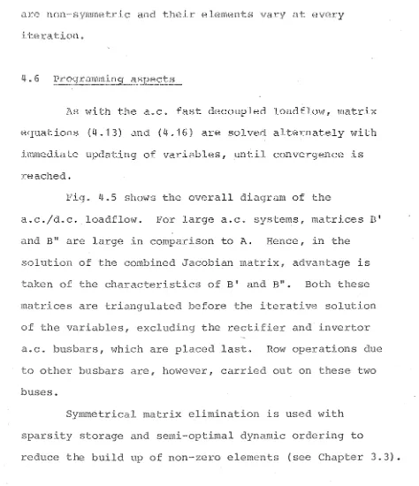
4.5 A.C./D.C. Jacobian matrix equations 81

4.5.1 Modified B" ma'trix equation 83

4.5.2 Modified B' matrix equation

Paqe

L[. 6. '1 Solut.ion of non~symmetj::Lc

-matrix equations 90

4.6.2 Solution technique when terminal

busbar voltages are specified 94

'-~. 7 Hes ul ts L~. 8 Conclusions

CHAprrER 5. A. C. /D. C. LOADI:'L01illS \'1ITH HEl-\LIS'I'IC REP HESENTATION OF THE CO"N"VERcrOR PLANT

5.1 Introduction

5.2 Sys-tem under consideration 5.3 D.C. system equations

5.3.1 Control specifications

5.4 Unified loadflow solution 5.5 Three terminal operation 5.6 Results

5.7 Conclusions

CHAPTER 6. GENERAL CONCLUSIONS

ACKNOWLEDGE~mNTS

REFERENCES A.PPENDICES

1 Derivation of the Jacobian elements of Newton's method

2 Gaussian-elimination and back-substitution

3 Algorithm for the triangulation of a symmetric matrix B using semi-optimal dynamic ordering

4 Modified back-substitution method for solving the matrix equation A = BX 5 Per-unit system and basic assnmpt:ions

for d.c. link model

97

104

106 -\06 -107

113 115

12 'I

125

129

13l

133

134

APPENDICES (Cont1d)

6 Calcula'tion of comIHutation reactances for -the New Zealand system

7 Corn~ction of per-unit sys·tem

for d.c. link with different convertor voltage bases

8 Ordering of d.c. link residuals and variables for the New Zealand scheme

Z~BS'l'HAC'l'

'1'he development of loadflows dorivec1 from the basic Newton-Raphson algorithm is reviewed in this thesis with thefast,decoupled method emerging as the best in terms of reliability and computation speed. These, and storage requiremeni:s, are dependent on programming techniques I and

a versatile programme is developed in Chapter 3 using a sparse matrix storage me'thod along with a compa'tible,

semi-optimal dynamically ordered matrix elj,mination scheme. The same identification vectors are 1J,sedto loca'te elements of the admi t'tance and Jacobian matrices of ,the fast

decoupled algorithm.

(O{

For applications wheJ':e .kncore compu'ter s'torage is at a premium, a method is derived, also in Chapter 3, which uses a single Jacobian matrix for both real and reactive power mismatch equations. This gives only sligh,t

degradation in reliability.

The versatility of the fast decoupled loadflow is extended in Chapter 4 by including the representation of a basic h.v.d.c. interconnection, directly into the Jacobian matrices of the a.c. network. The combined a.c./d.c.

Jacobians are solved al,ternately as in the a.c. method, and i t is shown that the reliability, speed and storage

advantages offered by the basic fast decoupled loadflow are preserved for large systems.

Finally in Chapter 5, a comprehensive d.c. link

and operating conditions encoun'tered in practice.

The New Zealand a.c.-d.c.-a.c. scheme is used as a test system, and results show convergence for all practical operating conditions wi th01.rt increasing the number of

i teraU.ons.

(a) General:

[A] [B] [ X] a

b

x

f (x) [ J]

a.c. d.c. h.v.d.c. o.l.t.c. p.u. r.m.s.

LI~;'r OF PRINCIPAL SYI1BOLS

denotes a matrix or vectoi transpose of matrix or vector inverse of a square matrix constant vee-tor

coefficient matrix

variable or solution vector elemen't of constant vector element of coefficient matrix element of variable vectoD func-tion of variable x Jacobian matrix

alternating current direct current

high voltage direct current

on load tap changing (transformer) per unit

root mean square

(b) A.C. system:

Sk

=

-

Vk

L'~k

k complex nodal voltage (polar co-ordinates)

=

Zkm

--e +jf

k k

~ _m +jX_{J ,em}

complex nodal vol'tage

y] _.;:m

k l:.Q _'-k.

e

.-km N M s mwk msk sp

*

G +jB km -km

8 -8

k In

branch admi~tance real power mismatch reactive power mismatch

voltage phase angle difference a.cross network bra.nch

number of system nodes

number of vol-tage controlled buses slack bus index

viii

denotes a bus m directly connected to k as for mwk but includes the case m

=

complex conjugate

(c) D.C. system:

v~

VI1

E/J.

a, t

x

x ,

m

n

m, n

nodal voltage (phase angle referred to slack node) nodal voltage (phase angle referred to convertor current)

convertor a.c. voltage direct voltage

alternating current direct current

alternating current (phase angle referred to convertor current on adjacent pole)

transformer ratios

convertor control angle-d.c. line resistance d.c. residual

d.c. link variable commutation reactances

IN1'RODUCTION

'1'he most importa.nt and widely used me'choc1 in Ne-twork Analysis is t_he loadflow (or: powerflow) which giv(::;s a

solution of the static operating condition of an electric power transmission system. By performing the loadflow, the engineer gains complete voltage and power information about the system 1.1nder the specified load conditions; power flow in lines and at busbars, in both magnitude and

direction, the voltage profile of the system and losses in lines, transformers, and total system losses.

Loadflow studies are performed in thre0 major areas of pOVler system c1evelopm(~ni: and operation.

(i) Pla:r~.E~i_~g: 'l'his is the future development of a system in which loadflows are used to study the effects and feasibility of changes in network configuration such as the removal or addition of lines, new generation units, or

increased loads due to a growing consumer demand. Load-flovl is central to the stability analysis performed on the proposed system. System security is also determined and mUltiple loadflows are performed -to evaluat.e contingencies.

used to evalu'l.t~,,::: thes(~ chan'J"cs and compensat:e for 11i9'h or low bus voltages by the addition or removal of static capacitors, the altering of ratios of transformers or by changing the reactive power of synchronous condensers or c:renera t.or uni ts " Stability analysis and system security s·t:udies ace also performed.

(:Lll.) ~~cono~J:_~_.2pe_Fa.!:Lon: As loads change

throughout the day there is a need to determine the best generating pattern to minimize costs of operation and provide the best voltage regulation. Loadflow is used to obtain the optimum settings of transformer taps, shunt capacitance and unit generation; subject to the operational constraints of equipment in the system.

The basic nurnerical algorithm for steady state a.c. loadflow has been almost fully refined to give reliable and accurate solutions of t,he state of a power system network. However, the success of the loadflow in terms of speed and s·torage requirements is largely depende.n·t on the computing techniques used by the programmer. In particular, the

2

input of system data and the formation of the network

configuration are as time consuming as the actual solution procedure, and efficient means of data storage and retrieval are required.

requirements of the basic algorit~u.

This thesis looks at the nunted_cal alqori i:hms derived from the successful Newton-Raphson method, and contributes to the development of loadflow by outlining a method of network data storage and manipulation, and the inclusion of an h.v.d.c. link into an a.c. loadflow algorithm.

The thesis is divided into four main sections: In Chapter 2 the formal Newton-Raphson method is presented along with the computational techniques of sparsity programming, optimally ordered triangular

facto~ization and an effective starting process, which have made -this method highly competitive with all other loadflow

algorithms.

The nodal iterative, Z-matrix and non-linear

prograrmning techniques are bypassed aB the development of these has been fully documented elsewhere anr'l because -these algorithms have not met with the success of the Newton-Raphson method.

By using the approximations; that the real power/ voltage angle and reactive power/voltage magnitude

relationships of a practical power system are only loosely coupled; the decoupled Newton loadflows have been developed with reduced Ja.cobians. By taking the approximations still

further, based on the physical characteristics of the system, the fast decoupled loadflow emerged in which the Jacobian matrices are constant valued and hence need -triangulation once only per network f instead of every

and computation time of the various methods evulved are discussed in this section.

'-rhe fe-tst decoupled algorithm is only as good as its computing techniques and Chapter 3 looks a-t a method of combined storage for the network admittance matrix and the Jacobian matrices. Details are given of a method of matrix' t.riangulation wi t:h semi~op-timal ordering I

compatible with ·the da-ta storage m,et:hod.

A Newton-like back-substitution technique, which has been used with the formal Newton method, is applied to the fast decoupled algorithm. In ·this the residual

vector is updated after each variable increment is obtained. Finally, to reduce storage requirement~a single

Jacobian matrix is used. Different aspects of network

models are suppressed to find a suitable matrix ""hich gives the most reliable convergence.

Chapter 4 develops a new met.hod for the inclusion of an h.v.d.c. transmission link into an a.c. loadflow. A basic, two terminal d.c. link model is described which includes a.c. busbars with filters, two winding o.l.t.c. transformers, convertors and the d.c. line. The d.c. link equations are solved simultaneously with the power

CHAP'l'ER 2

r.OADFLOWS FOn A, C. SYS'rEMS - 'rEE NETq'rON<-< R,l\PHSON )\lETHOD

AND APPROXIMATE 'I'ECHNIQUES DEHIVED FRGrI[ THIS

2.1 Introduction

The more successful methods of loadflow solution are based on the admittance matrix [V] representation of a

system(1). The advantages gained are ease of problem and data preparation and changes made to the system do not involve the recalculation of all nehvork elements. The admittance matrix is sparse for a practical power system, i.e. i t has only a few non-zero elements for large systems.

By contrast the impedance matrix [Z] of a system (which is the inverse of <the admi<ttance matrix) is full, and changes in system configuration affect the whole of the matrix(2) .

The first practical digital solution methods for loadflow were the Y matrix--itera<ti've methods, These were suitable because of the low storage requirements, but had the disadvan'tage of converging slm'lly or not at all.

Z matrix methods were developed which overcame the

reliability problem but a sacrifice was made of storage and speed with large systems.

The Newton-Raphson method was developed ~t this time and was found to have very strong convergence. I't was not I

hO""eVE.~r I ma.de competitive unti 1 spar.'sity progn_unrning and

optimally ordered Gaussian-elimination were introduced, which reduced both storage and sol ul:.iontime.

Non·-linear programming and hybrid me-thods have also been developed, but these have created only academic interest and have not been accepted by industrial users of loadflow.

The current problems faced in the development of loadflow are: an ever increasing size of systems to be solved, on-line applications for automatic control, and

system op·timization. Newer and modified me-thods of loadflow have been developed.to overcome these problems.

Five main properties are required of a loadflow solution method.

(i) High computational speed. This is especially important when dealing with large systems, real time

applications (on-line), multiple case loadflows such as in system security assessment, and also in interactive applications.

(ii) Low computer storage. This is important for large systems and in the use of computers with small core storage availability, e.g. mini-computers for on-line application.

(iii) Reliability of solution. It is necessary that a solution be obtained for ill-conditioned problems, in outage studies and for real time applications.

representati.ons of power system apparatus), and its

suitability for incorporation into more complicated

processes.

(v) Simplicity. ~he ease of coding a computer

programrne of the 10adflow al~Jor:':L thrn.

The type of solution required from a loadflow

also determines the method used:

accurate or a.pproximate

unadjusted or adjusted

off~line or on--line

single case or multiple cases

The first column are requirements needed for considering

optimal loadflow and stability studies, and the second

column those needed for assessing security of a system.

Obviously, solutions may have a mixture of the properties

from ei-ther column.

Alt-hough the Y mat.rix i terati ve methods were widely

used in practice, they have been gradually replaced by the

Newton-Raphson method and techniques derived from this

algorithm, which satisfy the requirements of solu.t.ion typf.!

and programming proper-ties. '1:11e hi storical deve lopmfm:t of

the Y matrix, Z matrix, non-linear and hybrid techniques

has been fully documented ( 3 4 5 1 ) I " and this sect.ion will

be confined to the Newton-Raphson techniques.

In power system analysis there are four variables

P

k -~. :ceal or active power

Q

k -- react.i ve o:c qlJ.aclrature power

V

k .. - voltage rnagnit.:ude 8

k - voltage phase angle

Only two are known a priori to solve the problem, and the aim of the loadflow is to solve the remaining two variables at a bus.

We define three different bus conditions based on the steady state assumptions of constant system frequency and constant voltages, where these are controlled.

(i) Voltage controlled bus. The total injected active pmver P

k is specified, and th~ voltage magnitude Vk is mainl~ained at a specified value by reactive power

injection(2,3). This type of bus

gen~rally

k is fixed by turbine governor setting and V

k is fixed by automatic voltage regulators acting on the machine excitation; or a bus where the voltage is fixed by supplying reactive power from static shunt capacitors or rotating synchronous compensators, e.g. at substations.

(ii) Non-voltage controlled bus. The total injected power, Pk+jQk' is specified at this bus. In the physical power :3ystem thi s corresponds to a load centre such as a city or an industry, where the consumer demands his power requirements. Both P

k and Qk are assumed to be unaffected by small variations in bus voltage.

10

choose one of the available volt:age control1(~d buses as slack, and too regard its ac Live powE~r as u,nknown.

The slack bus voltage is usually assigned as the system phase .1'e :Eerence I and its complex voltage

Ec-, :::: V ,~

Le

'" .::> u

if:'> there fore specified. The analogy in a practical power system is the generating station which has the reE.;ponsibility of system frequency control.

Loadflmv solves a set of simultaneous non-linear

algebraic power equations for the two unknown variables

! e 1 1 · a sy c:te_m ( 6 , 7 , 8) .

a':. ac 1 noc e ll1 ~. A second set of variable

equa'tions, which are linear, are derived from the first set, and an iteration method is applied to this second set.

The basic algorithm which loadflow programmes follow is depicted in Fig. 2.1. System data, such as bus bar power

condi tions, ne'twork connect.ions and impedance, are read in and ,the admit-tance matrix formed. Initial voltages are

specified to all buses; for base case loadflows, P,Q buses are set to 1+jO while P,V busbars are set to V+jO (2),

The iteration cycle is terminated when certain

criteria are satisfied. These may be when power mismatches for all buses are less than a small tolerance,

n

1, or

( 3)

voltage increments less than n2

_'.

n

n

'rhe sum of the square of the absolute values of power

mismatches is a further criterion sometimes used(9).

When a ::,olution has been reached, complete terminal

condi tions for all buses is computed. Line power flows and

[

Initialize Voltage profile

r - - - + >

1

-Calculate increments in bus voltage based on pmver mi sma tche s

Upda·te bus Voltages

Yes

Calculate complete terminal conditions

for all buses

L

~lve

losses and system totals

-J

12

The generalized Newton-Raphson method is an iterative algorithm for solving a set of simultaneous non-linear

algebraic equations in an equal nlffi1ber of unknowns ('1) •

for k=1--+N

m= 1--+N

(2 • 1 )

For simplicity consider one equation in one unknown. Let x P be an approximation to the solution, with error ~xP at iteration p (3). Then

(2.2)

This equation can be expanded by 'raylor' stheorem (10) ,

:2

:= f(x P )

+~xPf(xP) +iQ~~)

If the initial estimates of the variable x P is near the solution value f ~xP will be relatively small and all -terms

of higher powers can be neglected(11). Hence,

or,

=

'l'he new value of the variable is then ob-tained from p+1

x

₌

Equation (2.4) may be rewritten as

:=

(2 • L~ )

(2.5 )

(2 .6)

'The me-thod is reacH ly extended -to thQ SGt of N

equations in N unknowns. J becomes the square Jacobian

matrix of first ord~r partial differentials of the functions

fk(x ). Elements of [J] are defined by

In

J" ==

km (2 • 8 )

and represents the slopes of the tangent hyperplanes which

approximate "the functions f

J \. (x ) at each it_era tion poin-t m (1) •

The Newton-Raphson algorithm vI,il1 converge ifi

the functions have continuous first derivatives in the

neighbourhood of the solution(9) , the Jacobian matrix is

non-singular, and the initial approximations of x are close

"to the actual solutions. However -the method is sensitive to

the behaviours of the functions fk(x ) and hence to their m

formulation ( 1). The more linear -they are, the more rapidly

and reliably Newton I s method converges. Non-·smoothness,

i.e. humps, in anyone of the functions in the region of

in-terest, can cause convergence delays, total failure or

misdirection to a non-useful solution.

2.3.1 Equati?ns relating to power system loadflow

1 I , k ' t ' (12)

Tle non- lnear networ" governlng equa-lons are

Ik

=

mf;:k m

where Ik is the current injected into a bus k. The power

at a bus is then given by

Sk == Pk+jQk == Ek

1k

*

== E _k E Y_km *E

*

Mathematically speaking! the complex loadflovl equations are non-analytic, and cannot be differentiated in complex form(1). In order to apply Newton's method, the problem is separated into real equations and variables. Polar or rectangular co-ordinates may be used for the bus voltages. I-Ience we obtain two equations

or P(e,f)

and Q

k ::::: Q (V, e) or Q(e,f)

The differences in bus powers are obtained from(2) ,

=

=

and the increments in vol t.age are ob-tained from the

b ' , " 1 d' (3)

Jaco lan matrlx equatlons ln po_ ar co-or lnates

(7 1 3) or in rectangular co-ordinates -'

6P S T

{~

c.-.... _ _

6Q

=

u

6V2 EE FF

'

-The representation of the loadflow equations and the derivation of the Jacobian ma-trix elements are given in Appendix 1.

(2.'11a)

(2.11b)

(2.'12a)

(2. 1 2b)

For voltage controlled buses, V is specified, but not the real and imaginary components of voltage, e and f. Approximations can be made, for example, by ignoring the off-diagonal elements in the Jacobian matrix, as the diagonal elements are the largest. Alternatively

for the calculation of the elements the voltages can be cons ide red as E ::::: 1 + j O. The off-diagonal e :Lemen ts then become constant.

The polar co-ordinate representation appears to

have computational advantages over rectangular co-ordinat.es. Real power mismatch equations are present for all btlses

except the slack bus, while reac·tive pOltler mismatch

equations are needed for non-voltage controlled buses only, The Jacobian matrix has the sparsity of the

admi ttance matrix [YJ and has positional but not nWl1erical symmetry. To gain in computation, the form of [i18, i1V/V]T is normally used for the variable voltage vector (7) . Both increments are dimensionless and the Jacobian coefficients are now symme tric in structure. The values of [~J] are all functions of the voltage variables V and 8 and must be recalculated each iteration.

and V

k , -this non-linear term is numerically relatively small. Hence i t is preferable to use 6Q/V instead of 6Q in the Jacobian matrix equation(1) .

Dividing 6p by V is also helpful, but is less

effective since the real power component of the problem is not strongly coupled with voltage magnitUdes. A further

( 5 )

al-ternative is to fornn.11a~ce curr<~nt residuals at a bus .

I

=

k al _\:

+-

The Jacobian matrix equation becomes

'16

(2.13)

The off-diagonal terms of [J] then become constant in value and only the diagonal elements change each iteration (9) .

An approximation to the polar co-ordinate

representation is to neglect off-diagonal terms, giving rise to a banded Jacobian ma-trix. The voltage connection at a bus is then due to that bus only, all other bus

voltages are effectively held constant. While computation-ally simple, this method shows poor convergence in the same way as Y matrix iterative methods.

Th eore lca presena lons t ' 1 t t' h ave been developed(14,15) which show the Newton-Raphson technique as a-special case of a more general equation form. The similarities and differences to other loadflows are in the defining of factors in the equations.

PIG. 2.2 Flow diagram of the basic Newton~·Raphson

loadflow algorithm

[

Read in nebvork and terminal data

.--....-..-~----"'....-..,.~-~~---~-~~~~~~~~-J

Formulate vec-tors or arrays for network representation

,!.

C

-~~- ini-tialb~sJ

voltages Vk

ffi

-~--'

----~-~---Calcula-te bus powers pP and QP

_ k k

Calculate bus power mismatches pP and QP

k k

and Jacobian elements

1---,---Yes

- - - >

I

soi;:<~:;~~l

t

,

-Upgrade vol-tages

e

_e

_6e

k k k

2.3.2 Tecl2ni.sc~~e.:~ __ ~vlli.ch m~~;~_~he _~::=:~~_~co..!~·-R~0.2.§?n

!~c:.thod COJ'::!J?_et=!:..~i VE~ _.~~.J_oa9flow

For most power sy::;tenl network s the admi t-tance matrix is relatively sparse, and in the Newton-Raphson method of loadflow the Jacobian matrix has this same

sparsity. The techniques which have been used to make

the Newton~Raphson competitive with other loadflow methods

involve the solution of the ,Jacobian matrix equation and the preservation of the sparsity of the matrix by

optimally ordered triangular factorization. 2.3.2.1 Sparsity progranrrning

18

In conventional matrix programming, double subscript ( 16)

arrays are used for the location of elements • with

sparsity programming, only the non-zero elements are stored, in one or more single veci.-:ors, plus integer vectors for

identification.

For the admittance matrix of order n the conventional storage requirements are n2 words, but by sparsity

programming 6b

+

~

2.3.2.2 Triangu~ar factorizati.on.

To solve the Jacobian matrix equation (2.120.), represented here as

[ J] [6E] (2.14)

inverse of [J] and solve for [~E] from

[l1E] [J] -1 [l18] (2.'15)

In power sys'tems [J] . (17 )

mat.rlX .

is usually sparse but [J] -1 _{is a full}

The method of triangular factorization solves for ,the vector [l1E] by eliminating [,J] to an upper triangular matrix with a leading diagonal, and then back-substituting

for [l1E] (16) .

i.e. Eliminate to [ l1 S 1] == [ U] [ l1E ] and Back-substitute [U]-l [l18']

=

The triangulation of the Jacobian is best done by rows(12). Those rows below the one being operated on need not be entered until required. This means that the maximum

storage is that of the resultant upper triangle and diagonal. The lower triangle can then be used to record operations.

The number of multiplications and additions to t _{rlangu a e a . u} · 1 t f 11 _{ma rlX J.s} t ' .

3"

the inverse (17) . with sparsity programming t.he number of operations varies as a factor of N. If rows are normalized N further operations are saved.

2.3.2.3 Optimal ordel.-:.ing

20

~rhe pivot elemen-t is select.ed to minimize t:he accumu1at:ion of non~zero t:erms, and hence conse:cve sparsity, rather than minimizing round off error. Th e d ' lagona s are use 1 d ' as plvots (12,18) .

Optimal ordering of row eliminations to conserve sparsity is a practical impossibility due to the complexity of programming and time involved. However I sem:L~op·timal

schemes are used and these can be divided into two sections. (a) Pre-orderinsr. Nodes are renumbered before

triangulation(16). No complicated programming or storage is required to keep track of row and column interchanges. (i) Nodes are numbered in sequence of increasing number of connected lines.

(ii) Diagonal banding - non-zero elements are arranged about either the major or minor diagonals of the matrix.

(b) Dynamic ordering. Ordering is effected at each row during the elimination.

(i) At each step in the elimination, the next row to be operated on is that wi·th the fewes·t non-zero terms.

(ii) At each step in the elimination, the next row to be operated on is that which introduces the fewest new non-zero terms, one step ahead.

(iii) At each step in the elimination, the next row to be operated on is that which introduces the fewest new non-zero terms, two steps ahead. This may be e~tended to the fully optimal case of looking at the effect in the final step.

divided into groups which are then optimally ordered. This is most efficient if the groups have a minimLIDl of physical intertie. The matrix is then anchor banded(18) .

The best method arises from a trade-off between a processing sequence which requires the least nlIDlber of

t ' d ' ~ , ( -19)

opera lons, an tlme ano memory :reqluremen·ts .

The dynamic ordering scheme of choosing the next row to be eliminated as that with the fewest non-zero terms, appears to be better than all other schemes in sparsity

conservation, number of ari-thmetic operations required, ordering times and total solution time(16).

However, there are conch tions under which other ordering would be preferable, such as system changes affecting only a few rows which are numbered las·ti the

matrix is only slightly non-symmetric - put ·these rows last, or if a network is composed of subnetworks wi·th relatively few interconnections - then use cluster ordering.

2.3.2.4 Starting processes for the Newton-Raphson method Convergence of the Newton-Raphson algorithm is dependent on a good starting approximation of bus voltages, close to the final solution for the system. A bad starting value of variables leads to divergence, slow convergence or convergence to a wrong solution.

In power system loadflow, setting voltage controlled buses to V -I- jO and non-voltage controlled buses to 1

+

may give a poor starting point for ,the Newton-Raphson method. If previously stored solutions for a network are available these should be used. One or two iterations of 0_

the Newton method. This shows fast initial convergence unless the problem is ill-conditioned, in which case

( 'I )

-divergence occurs .

A more reliable method is the use of one iteration of a d.c. loadflow to provide es-timates of voltage angles;

22

followed by one iteration of a similar approximate technique to obtain voltage magnitudes (20) . The total computing time for both sets of equations is about 50% of one Newton-Raphson iteration and the extra storage required is only in the

programming s-t:atemen-ts. The resulting combined algori-thm is faster and more reliable than the formal Newton method and can be used to monitor diverging or di~ficult cases, before commencing the Ne\"ton-Raphson algorithm.

2.3.3 Characteristics of -the Newton-Raph?on loadfl?w With sparse programming techniques and optimally ordered triangular factorization, the Newton method for solving loadflow has become faster than other methods for large systems. The number of iterations is virtually

characteristic of convergence (12) . Most systems are solved in 2 --+ 5 iterations and no a priori knowledge of acceleration

(,15 )

factors is necessary •

With good programming the time per iteration rises nearly linearly with the number of system buses N, so that the overall solution time varies as N. One Newton iteration is equivalent to about seven Gauss-Seidel iterations. For a 500 bus system, the Gauss-Seidel method takes about 500

then 15:1. Storage requirements of the Newton method are greater, however, but increase linearly with system size and is therefore attractive for large systems(20).

The Newt.on metJ10d is very reliable in system solving f

given good starting approximations. Heavily loaded systems with phase shifts up to 90° can be solved and the method is not troubled by ill-conditioned systems, or critical of slack bus location.

Due to the quadratic converg-ence of bus voltages, high accuracy (near exact solution) is obtained in only a

few iterations. This is important for the use of loadflow in short circuit and stability studies. The method is

readil~ extended to include tap changing transformers,

variable constraints on bus voltages, and reac-tive and

optimal power scheduling. Network modifications are easily made.

The success of the Newton method is critical on the formulation of the problem-defining equations(1). Power mismatch representation is better than the current mismatch versions. 'ro he lp nego-tiate non-lineari ties in the defining functions, limits can be imposed on the permissible size of voltage corrections at each iteration. These should not be too small, however, as they may slow down the convergence for well-behaved systems.

The coefficients of the Jacobian matrix are not constant, bu-t a:re functions of the voltage variables V and Sf and hence vary each iteration(8). However, after a few iterations, as V and 8 tend to their final values the

One modification to the Newton algorithm is to calculate the ,Jacobian for the firs't two or ,three iterations only and then use the final one for all the following iterations.

Alternatively the Jacobian can be updated every two or mm:e iterations. Neither of these modifications greatly affects the convergence of the algorithm, but much time is saved

(but not storage).

2. L! Decoupled Newt.on loadflow

An inherent characteristic of any practical electric power transmission system operating in the steady state

condi tion is the strong interdependence between active powers and bus vol tage angles t and be·tween reac·tive powers

and voltage magnitudes. Correspondingly, the coupling be'tween these I P-8 I and I Q-V' components of the problem

is relatively weak. Many algorithms have been proposed which adopt this decoupling principle (1 ,22).

'1'h e vo It age vec' ors t method(23) uses a serles .

approximation for the sine terms which appear in the system defining equations, ·to calculate the Jacobian elements

and arrive at two decoupled equations

[I]

=

[ J] = (2.16b)

where for the reference node 8

0

=

=

'1' kk

U

km

::=

k m

,--~---~---~

'7. 2

Ix

'-'km "km

2: T

mwk 'km

1

Z 2

Ix

km krn

I:

mwk

U krn

(2.'J7a)

(2.17b)

(2.17c)

(2.17d)

[U] is constant valued and need be triangulated once only for a solution. [T] is recalculated and triangulated each

iteration. The two equations (2.16) are solved alternately until a solution is Dbtained.

The equations (2.16) can be solved using Newton's method(24), by expressing the Jacobian equations as

~

l~l~

since [L1P] ::= _{[L1 I]}

and [ L1Q/V]

₌

T and U are defined in equations (2.17).

Equations (2.18) are defined as the 'voltage vectors and Newton's method', The values of K are small and can be neglected, then:

[L1P] [11'] (L18] (2.19a)

[I'1Q/V] [U] [L1V] (2.19b)

The most successful decoupled loadflow is that

based on the Jacobian matrix equation for the formal Newton rnethod (25) •

26

(2.20)

where the Jacobian submatrices H, N, J, L are defined in Appendix 'I.

If the sub-matrices Nand J are neglected, since they represent the weak coupling between 'p-O' and I Q-V' ,

we obtain the decoupled equations (26)

[L\P] :::: _{[H] [L\ 0] (2.21a)}

t

It has been found ·that: the latter equa·tion is relatively unstable at some distance from the exact solution due to the non-linear defining functions. An improvement in convergence is obtained by replacing this with the polar current-mismatch' formulation(25)

[L\ I] [D] [L\ V] (2.22)

Al ternati ve ly the right hand side of both equations (2.21) is divided by voltage magnitude V

.~

[L\P IV]

--

[L\Q/V]

=

They must be calculated and triangulated each iteration. Further approximations that can be made are to

,

assume that E] :::: '1.0 r). u., for aLL buses rand G

J «B, in

< 1: <m J<.m

calculating the Jacobian elements(26). The off-diagonal terms t.hen become symmetric about the leading diagonal.

The decoupled Newt,on method compares very favourably wi th the formal Newton me-thod. Whi Ie re liabi Ii ty is just as high for ill-conditioned problems, the decoupled method is simple and computationally efficient. Storage of the

,Jacobian and matrix triangulation is saved by a -factor of 4, or an overall saving of 30-40% on the formal Newton load-flow (25), Computation time per iteration is also less -than the Newton me-thod (27) •

However f the convergence charac'teristics of the

decoupled method are linear, the quadratic characteristic of the formal Newton being sacrificed(1). Thus, for high accuracies, more iterations are required. This is offset for practical accuracies by the fast initial convergence of the method. Typically, voltage magnitude s converge to vIi thin

o

inclusion of transformer taps, phase shifters, interarea power transfers, Q and V limits) 'take many more iterations.

An attempt to offset the degraded convergence

characteristics of -the formal Newton loadflow,' dneto the decoupling principle, results in a general equation form of

28

== (2.2LI)

where E: - 1 for i::he full Newton-·Raphson method E - 0 for the decoupled Newton algorithm

A Taylor series expansion of the Jacobian about

E

=

Newton-Raphson rnethod whereas -the decoupled method is a zero order approximation. The method has quadratic convergence properties because of the coupling, but retains storage requirements similar to that of the decoupled method.

2.5 Fast decoupled loadflow

By further simplifica-tions and assumptions, based on the physical properties of a practical system, the Jacobians of the decoupled Newton loadflow can be made

constant in value. This means that -they need be triangulated only once per solution or for a particular network.

For ease of reference, the real and reactive power equations at a node k are reproduced here.

where 8

km

V

m sin 8k m -- Bk pm cos 8] (In )

(2.25a)

(2.25b)

sin

°

3

-.

-6

cos

e

-

2

'2

The equations, over all buses, can be expressed in their simplified matrix form

[A] [0]

=

[C] [V] :::: [Q] (2.2Gb)

where P and Q are terms of real and reactive power respectively and

Akk :::: V_k L: V Bkm mUlk m A

km == -V k V m Bkm m

t

kk == _mUlk L: t km B km C

km ==

-

f.

km - tap ratio if a transformer is in Lhe line. A modification suggested is to replace the firs·t equation

(2.26 a) by

A 1\ A

[A] [ 0] == [P]

A

m

=!

where A = - B

km km

A

Akk

=

1\

Ok == Ok • V_k

Hence [A] becomes constant valued.

A similar direct method is obtained from the

. (24)

30

If V

m, Vk are put. as 1.0 p" U. foL' the calculation of mat.rix [T], then [T] becomes constant and need be triangulated once only. 'This same simplification can be used in the decoupled voltage vectors and Newton's method of equations (2.19).

Fast decoupled load flow algorithms are also derived from the Jacobian matrix equations of Newton's method,

equations (2.20) I and the decoupled version, equations (2.21).

f J h . (26)

I we maze t e assumptlons (i) _E

k , Em

=

k , and hence can be ignored (for most

{m m

transmission line reactance/resistance ratios,

~

»

.

(iii) cos (e

k - em) '1.0 sin (e] - e )

=

, { m

since angle differences across transmission lines are small under normal loading conditions.

This leads to the decoupled equations [liP] [13] [lie]

[IIQ] :=

where the elements of [~] are

=

mwk

B

km

of order (N - 1) of order (N - M)

for m t- k

(2.27a)

(2.27b)

and B] are the imaginary parts of the admittance matrix.

(IU

To simplify still further, line resistances may be neglected in the calculation of elements of

[~]

An improvement over equations (2.27) is based on the decoupled equations (2.23) which have less non-linear

[6P/V] [B*] [68]

[6Q/V] [B*] [6V] (2.28b)

A number of refinements make l:his method very successful: (a) omit from the Jacobian in equation (2.28a) the representation of those netv.JOrk elements that predominantly affect: MVAR o:r" react-:.ive power flow, e.g. shunt reactances and off-nominal in-phase transformer taps. Neglec·t also the series resistances of lines.

(b) omit from the Jacobian of equation (2.28b) the angle shifting eff~cts of phase shifters.

The resulting fast decoupled loadflow equations are then,

where

[6P IV]

=

=

B" km

=

=

=

=

1 - X

k; 1 l:: X mwk km

- B _km

l:: Bk m().lk m

(2.29a)

(2.29b)

for m

f:.

for m

f:.

The matric(:~s B' and B II are real and are of order

(N - 1) and (N - M) respectively. B II is symmetric in value

and so is 15' if phase shifters are ignored; i t is found that t-:.he perfo:r"mance of the algorithm is not adversely

32

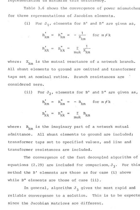
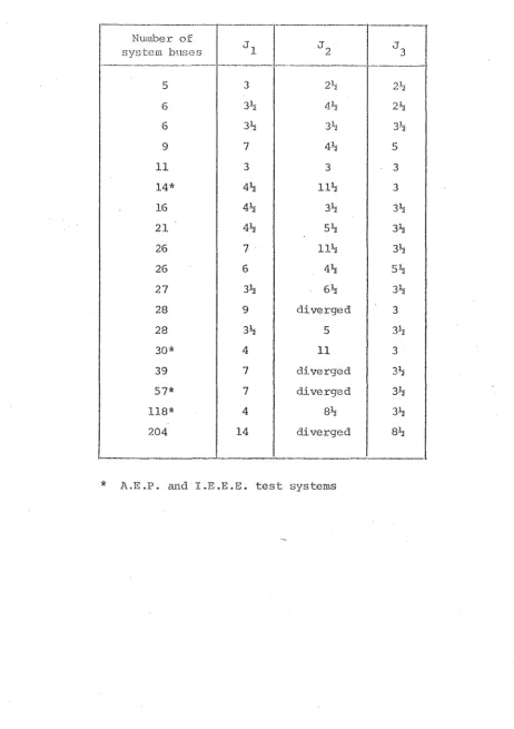
for a net.work.

Convergence is geometric I 2 - 5 i terat.ions are

required for practical accuracies; and more reliable than the formal Newton's method. This is bE~cCluse the (~lements of B I and B" are fixed approximations to t:he tang-ents of the

defining functions 6P/V and 6Q/V, and are not susceptible to any 'humpsi in the-defining functions.

If 6P/V and 6Q/V are computed efficiently, then the speed per iteration of the fast decoupled method is about five times that of the formal Newton-Raphson or: about two thirds that of the Gauss-Seidel method(1,30,27). Storage requirsments are about 60% of t.he formal Ne~ton, but slightly more than the decoupled New-ton method.

Changes in system configuration are easily effected, and while adjusted soltreions take many more i-ceracions

these are short in time and the overall solution time is still low.

CHAPTER 3

COMPUTING TECHNIQUES USED IN A FAST DECOUPLED A.C.

CONVERGENCE AND REDUCING SrrORAGE

3.1 Introduction

In Chapter 2 the development of the Newton-Raphson loadflow, and the methods derived from. it, have led to a very efficient and powerful method in the fast decoupled loadflow given by equations (2.29). However, the complete success of this method relies heavily on programming techniques which must take full advantuge of the characteristics of the

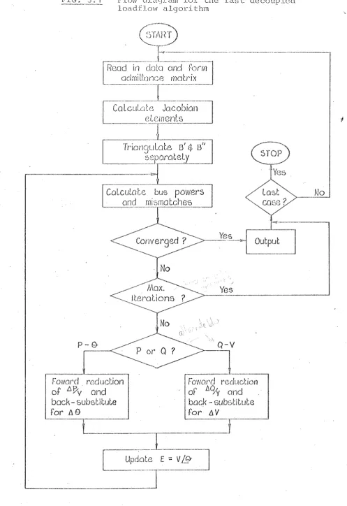
constant Jacobians, in line with the physical characteristics of the power system network. A simplified flow diagram of the fast decoupled method is given in Fig. 3.1.

Th ' lS C h apter d escrl es 'b th e a ap a lon d t t' 0 f L' k In ne t(32) ,

a sparsity storage technique, for use in the fast decoupled loadflow, and a compatible, semi-optimal, dynamically ordered elimination scheme used for the tri~ngula·tion of the Jacobian matrices.

Attempts have been made at improving the convergence of the fast decoupled algorithm by a method of upda'ting

FIG. 3.1 F:Low dia<]J:,am fo.1:' the fas't c1ecouplod loadflow algorithm

No

"'",---.,

""'- Convetged

?

---,

, No

" ./

Max,

.

Ye.s

<---)terotion5

~---'

~-No

p- 0-

,

Q-V

Po~--~

__

Fowot"d reduction

FO'Ncwd

of /::,

t?v

and

or

ond

back- substitute back - substitute

for

for

---c--='--r-'·---'---j

[

---Urd~tf; ~

::

LC?--]'

. - - -

Linknet is a structure for the computer representation and solution of network problems, by means of indirect addressing of elements which represent the network. Applied to power systems (33) , the nodes and branches of a network are numbered either manually or by the computer. Node (bus) and branch

properties of the system, e.g. self and mutual admittances, are stored in one-dimensional vectors and each position in these vectors is identified with the node or branch having the corresponding number.

Each branch has two ends and can be obtained from, ENDA ::; 2. BR~NCH -1

ENDB ::; 2. BRANCH

where ENDA, ENDB and BRANCH are integers in Fortran IV programming language. Conversely, a branch may be derived from either of its end numbers using

BRANCH ::; (END

+

which applies integer round off to obtain the two to one mapping between ends and branches.

The network topology is defined by constructing a linked - list of branch ends connected to each node.

rrhis is illustrated for a small network in Fig. 3.2.

For each node a pointer LIST(NODE) is defined, which indicates the end of the first branch connected to NODE.

FIG. 3.2

NODE

1

2

3

4

The LIST (NODE) , NEXT (END) and FAR(END) pointers for a network

LIS'l' (NODE)

LIST (NODE) EtID NEXT (END) FAR (END)

1

)- 2

- - -

-

-8

4

1 3

2 - - - ) - 5

; '

3 ; ' .- 0

.-4 ; ' 6

.-5" _{~ 7}

,.

6

_,.

7 "::- ) ₀

8 0

2

1

4

1

4

2

3

2

The arrows indicate the linked list of branch ends

connected to node

(2).

The last branch end connected to NODE is indicated when

NEx'r (END) == O.

These two pointers uniquely define the neb-york topology. All the branches connected to a node can be obtained using the procedure.

Initialize then set and

END

BRANCH

END

LIST(NODE) (END + 'I) /2

=

=

o.

In power system analysis i t is important to know the nodes directly connected to a specified node. For this convenience a ·third point.er FAR (END) is defined which indicates the node at the opposite end of -the branch.

'1'he node s connected to any given node can now be obtained using the procedure

Initialize END

=

=

and END

=

=

o.

equivalen-t of the admittance matrix, self admittances are stored as node data while mu·tual admittances are stored as branch data.

3.3 Triangulation of Jacobian matrices for nodal elimination

3.3.1 §,olutioE of...2en.~£a~~ matrix equation For a matrix equation

3B

the solution vector [X] is obtained by triangulating the matrix [B], augmented by [A]; and -then backc-substi t.ut:ing for the variables [Xl.

Consider equation (3.1) written fully as

i-~--'~-""-l---"----~"--r~~

b

11 b12 b1n

x

2 ( 3 • 2)

1

a

n x n

Eliminating x

1 from all rows except the first, we obtain

1 1 1

a

1 b11 b12 b1n X1

2

0 2 2

a

2

₌

2

0 b2 b2

a x

n n2 nn n

-~-~---where,

1

2 1 bk1 1

a

k == ak :;:-r _b a1 11

for k :::: 2 -to n

1

2

bi

b

k1 _bl

b

km

=

-

=

m .- 2 to n

(superscripts indica-te the order in which quan-ti ties are derived)

Similarly by using b~2 _{as t.he pivot elemen-t, we eliminate x 2} from all rows except the first and second. After n - 1

J a'i 2 a 2 n a n b

n

The varj,ables can now be obtained by back-substitution.

x n

( 3 • 4)

and the variables on successive nodes k - n-1, ... ,1, are

calculated from

(3.5)

Appendix 2 gives the solution for a 3rd order system.

Triangulation can be considered as a series of

network reductions in which ,the subnetwork of the

branches connected to a node is replaced by an equivalent

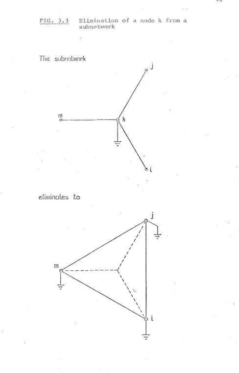
network as viewed from the adjacent nodes. The elimina'tion

of a node k from a subnetwork is shown in Fig. 3.3.

For a node m connected to k, b is changed to

rum

b ' _mm = b mm

and am is changed to

._. a m

The mutual term b . bet.ween nodes m and j becomes

In]

b ' .

ill]

=

( 3.6 )

(3.7)

FIG. 3.3 Elimination of a node k from a

s ubnetitlOr]{

The

eUminotes

to

/ /

/

m

/

€ - - -

---<

1

_-

\,

\

/

/

/

/ I

I

J

,

--\

\

,

,

_,

\

.

Il

If the mutual term between m and j \va.s p.reviously zero!

then a new branch is introduced into the equivalent network. With the Jacobian matrices B' and B" in the fast

decoupled loadflow, t:he elemen·ts are real and constant and the matrices need be triangulated once only per solution. In the computer programme, triangulation is considered separately from the reduction of the residual vectors ~P/V and ~Q/V and the back-substitution for ~8 and ~V, since the latter are performed every iteration.

The forward reduc·tion of the residual vec·tors, is performed by applying the same elimination operations used to triangulate B' and B". These operations have been

stored in the elements of the triangulated Jacobian matrices and their order by an integer vector. For back-substitution, nodes are operated on in the reverse order to that of

elimination, using the form of equation (3.5).

3.3.2 Use of the Linknet point.ers for tl}e adI1}j.·t.:t.?-nQQ and Jacobian matrices

Elements of the Jacobians B' and Bit are formed during the input of data. Because of posi·tional and value symmetry i t is only necessary to store the upper triangular terms along with the leading diagonals of these two mai::rices. Diagonal terms are st.ored as node data and off-diagonal

terms as branch data 1 and hence the Linkriet. method of storar;re

can be used for these matrices. More importantly, because the Jacobian matrices have the exact sparsity of the

admittance matrix, when considering all buses, the same

Ll2

In the triangulotion of B I and B" f new off"-diagonal

elements created can be represented as new branches. For every new branch, t~o new ends are added. The NEXT pointers of these new ends are set to the LIST pointers of the two nodes which the new branch connects (these are st6red in the new FAR pointers) and the LIST pointers are changed to the ne1l7 ends. Thus it is necessary to save -the LI~)T pointers of the original network and create new lists LISTP and LISTQ for -the B' and B" matrices respectively. The original form of the NEXT and FAR pointers is unchanged; i t is only added to. The resultant necessary integer pointers to repre~ent the admittance and Jacobian matrices are illustrated in Fig. 3.4.

Empirical results from twenty-four test systems have shown that the combined dimensions of the NEX~[, and FAR

pointers are such that

(0)

+

+

Total pointer storage requirements are then 3N

+

+

At any stage during the formation of the poin-ters during data read in, or during the triangulation of B' and

loadfloVl method

LIS l'

LISTP

LISTQ

NEXT

FAR

where

C~

-

+ N ---+

[ __

---'J

matrix

a'

[ - -

]

-

[

J--~~----J

L

__ r_(a_) _

I

--~

+---

(o)

-

(a) - pointers created by branches added in

a'

(b) - pointers created by branches added in

a"

All branches read as network data input are stored separately using the Linknet pointers. Since the same

pointers are used for the elements of the Jacobian matrices i t is necessary in effect to combine parallel branches, between the same nodes of a network, during the

triangulation of B I and B".

There are two operations to consider:

(i) change the off-diagonal term of parallel branches connected to a node k due to the elimination of a node i above k in ·the matrix. Terms are added only ·to the first branch called; the values of t.he other parallel branches remain unchanged.

For p parallel branches

B'

km

1

=

Bk,B,

B

+

km 1 _1< ' J _<. B" _{I I}

.•.. , B

km _p remain unchanged.

(3.9)

(ii) change the terms of rows below that which has parallel branches, due to the elimination of a node k

containing those branches. The values are combined, in effect, in a table YTAB and the elimination performed.

B*

_--

+

₊

+

km km

1 km2 km p

( 3 • '1 0)

*

and . _Bki I

₌

-

Bmm (3.1

n

or B~

1m B. 1m

*

B.] _,~(. Bk _m

- ' "

-~--..--.-B

kk

for i > k

which operates on elements in COlUll1l1 m below k.

(:L'12)

These operations do not change the forward reduction

and back--sub:3ti-tu-tion algorithm as terms are additive.

(i) Forward reduction of [AJ

A

In

B' A

km1 k

-Bkk

B* A km k

-Bkk

B kk

(ii) Back-substitution for [Xl

,

X

=

m m

:;::: X

m

B' X

km 1 k

-Bkk

In part (ii) of the elimination routine B

*

km

explicitly but this is not necessary in the forward

(3.13)

(3.14)

reduction of A or in the back-substitution for X. In the

latter two, the net effect of the summation of terms due -to

parallel lines is I how'ever I eguivalen't to using

Bj:m'

3.3.4 Ro~ ordering sui,table for fast decoup}e~Joa9flow

' - ,

Semi-optimal ordering schemes to minimize the

accmnula'tion of non-zero terms in the J'acobian during

triangulation have been discussed in Section 2.3.2.3,

wi tIl reference to formal New-ton-Raphson me-thods of 10adflow.

When considering the fast decoupled algorithm, the dynamic

that with the fewest non-zero terms becomes even more appealing compared to pre-ordering schemes.

Because of its lonce-offl _{nature of ordering}

the .Jacobian matrices, no advantaC:fe is gained by having the dynamic simulation outside the elimination procedure., In fact, computing time is reduced since the assessing of nodes and branches is not duplicated as i t is in separate ordering and elimination routines.

An algorithm for the triangulation of a syrmnetric ma-trix B is given in Appendix 3.

In Jacobian mat~ix Bt I the slack bus does not enter

into the triangulation, and in B" only non-vol-tage

controlled buses are present. It is convenient, however,

46

to have all buses represented in both matrices for cases where the slack bus designation may be changed or where

there is violation of voltage magnitude limits at load buses or reactive power limits at voltage con-trolled buses. An integer vector NSTATE is definedi a zero indicates the node can be elimina-ced, unity indicates that the node is

protected from elimination. The full representation of the ne'cwor]< does not affec-c the mathematics of the reduced

matrices B' and B", bu-t facilitates bus type changes. Table 3.1 gives an indication of the build-up of non-zero elements generated during the triangulation of Bt

*

+

TAB2=:~,_ 3.1 Generation of non-·zero elements during the t.ricmgulation

of the fast: decoupled Jacobian matrices using dynamic node ordering

--~~ -- - -

---(a) No. of system buses 14~' _30* 57'k _118* 191+ 341+

(b) No. of system branches 20 41 80 179 245 489

(c) _{Branches added during}

4 13 58 78

triangulation of B' 64 142

( d) Branches added qurlng

0 12 2~ 0

triangulation of B" 64 142

L: (b+c+d) 24 66 161 257 373 773

Ratio

-

a

Ratio L: (b.!c+d) 1.72 1.20 2.82 2.16 1.95 2.27

a

,

Ratio L: (b+c+d) 1.20 1.61 2.01 1. 44

b 1.52 1.58

A.E.P. and I.E.E.E. test systems