Solution of Electrohydrodynamic Flow Equation Using an Orthogonal Collocation Method Based on Mixed Interpolation

(1)

ISSN Online: 2327-4379 ISSN Print: 2327-4352

DOI: 10.4236/jamp.2018.63050 Mar. 26, 2018 573 Journal of Applied Mathematics and Physics

Solution of Electrohydrodynamic Flow

Equation Using an Orthogonal Collocation

Method Based on Mixed Interpolation

Shruti Tiwari, Ram K. Pandey

*

Department of Mathematics and Statistics, Dr. H.S. Gour Vishwavidyalaya, Sagar, India

Abstract

In this Paper, we have proposed a new weighted residual method known as orthogonal collocation-based on mixed interpolation (OCMI). Mixed inter-polation uses the classical polynomial approximation with two correction terms given in the form of sine and cosine function. By these correction terms, we can control the error in the solution. We have applied this approach to a non-linear boundary value problem (BVP) in ODE which governs the elec-trohydrodynamic flow in a cylindrical conduit. The solution profiles shown in the figures are in good agreement with the work of Paullet (1999) and Ghase-mi et al. (2014). Our solution is monotonic decreasing and satisfies

( )

1

0

1 w r

α

< <

+ ∀ ∈r

( )

0,1 , where, α governs the strength of non-linearity

and for large values of α solutions are O  _{ }_α1 . The residual errors are given in

Table 1 and Table 2 which are significantly small. Comparison of residual

errors between our proposed method, Least square method and Homotopy analysis method is also given and shown via the Table 3 where as the profiles of the residual error are depicted in Figures 4-8. Table and graphs show that efficiency of the proposed method. The error bound and its L2-norm with re-levant theorems for mixed interpolation are also given.

Keywords

Electrohydrodynamic (EHD) Flow, Weighted Residual Method, Orthogonal Polynomial, Mixed Interpolation

1. Introduction

The electrohydrodynamic flow (EHD flow) of a fluid in a “ion drag” configuration How to cite this paper: Tiwari, S. and

Pan-dey, R.K. (2018) Solution of Electrohydro-dynamic Flow Equation Using an Ortho-gonal Collocation Method Based on Mixed Interpolation. Journal of Applied Mathe-matics and Physics, 6, 573-587.

https://doi.org/10.4236/jamp.2018.63050

Received: January 18, 2018 Accepted: March 23, 2018 Published: March 26, 2018

(2)

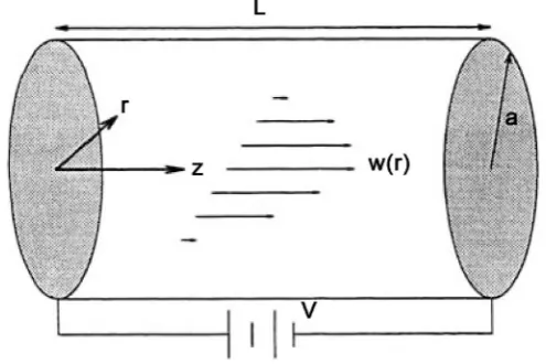
DOI: 10.4236/jamp.2018.63050 574 Journal of Applied Mathematics and Physics in a circular conduit (see Figure 1) is governed by a nonlinear second-order ordinary differential Equations ((1), (2))

2

2 2

d 1

1 0, 0 1,

d 1

d a

w dw w

H r

r r w

r α

 

+ + _ − _= < < −

 

(1)

subject to the boundary conditions

( )

0 0, 1

( )

0.

w′ = w =

(2) where w r

( )

is the fluid velocity, r is the radial distance from the center of the

cylindrical conduit, Ha is the Hartmann electric number and the parameter α measures the strength of the non-linearity. It has been noted that the nonlinearity occurred in this problem is in the form of a rational function and thus, creates a significant challenge in regard to obtain analytical solutions.

Though, some analytic solutions are introduced by several researchers which are mentioned here. In 1997, Mckee et al. [1] developed regular perturbation solutions of EHD flow Equations ((1), (2)) in terms of the nonlinearity control parameter α governing a nonlinearity of the problem. Mckee and his coworkers used a Gauss-Newton finite-difference solver combined with the continuation method and Runge-Kutta shooting method to provide numerical results for the fluid velocity over a large range of values of α. This was done for both large and small values of α.

For α1, Mckee et al. [1] assumes the solution of the form

( )

(

,

)

₀ n _n

(

;

)

n

w r =w r α =

∑

∞₌ α w rα and obtained the O

( )

α3 perturbation

solution as

(

)

0

( )

_{( )}

0

, 1 I Hr .

w r

I H

α = −

Similarly, for α1, the authors in [1] proposed that the solution of BVP (1 -

2) could be expanded in the series of the form

( )

0

(

;

)

n n n

w r =

∑

∞₌ α w rα with

( )

1

O leading term. In 1999, Paullet [2] proved the following the existence and

uniqueness of a solution of BVP of electrohydrodynamic flow.

[image:2.595.249.497.544.709.2]

For any α>0 and any Ha2≠0 ∃ a solution of BVP (1 - 2). Further this

(3)

DOI: 10.4236/jamp.2018.63050 575 Journal of Applied Mathematics and Physics solution is monotonically decreasing and satisfies 0

( )

1

1 w r

α

< <

+ ∀ ∈r

( )

0,1 .

Remark: Clearly the solution w r

( )

of BVP (1 - 2) satisfies w r

( )

1

α

< _and

( )

w r never equals 1

α, otherwise the term

( )

1 w r

w r

α

− creates the singularity.

Paullet [2] claimed an error in the perturbation solution and numerical solution given in [1] for the large value of α. This is obvious from the fact that for the large α, the solutions are of O 1

α

   

  not of O

( )

1 as proposed in [1]. For

1

α , our solution obtained by orthogonal collocation method based on mixed interpolation are in complete agreement with those of [1] and [2] but for α 1,

the proposed solution profiles are similar to those of [2]. The strong strength of our proposed method is its simplicity and high accuracy. Our results for large and small value of α are in good agreement with those of the solutions given in

[3] [4] [5]. Recently Mastroberardino [3] presented the approximate solution by

homotopy analysis method (HAM) for the nonlinear BVP of electrohydrodynamic flow Equations ((1), (2)) for α∈

[ ]

0,1 . In 2011, Pandey et al. [4] settle this

differentiation and they showed that the solution profile for the large value of α

is in good agreement with those of Paullet [2]. They solve EHD flow Equations ((1), (2)) using two semi-analytical algorithms based on optimal homotopy asymptotic method (OHAM) and optimal homotopy analysis method. They showed that HAM solutions are quite accurate especially for lower values of the parameters α and 2

a

H , but the accuracy decreases rather fast for higher values of

these parameters. They found that for the large value of α, solution profile given by Paullet was correct and the solution profiles given in Mckee’s paper was quite different with those given in [4]. Khan et al. [5] introduced new homotopy perturbation method to solve EHD flow equation. Recently, Ghasemi et al. [6]

introduced Least square method (LSM) to find the approximated solution of EHD flow equation.

The aim of the present article is to introduce a new weighted residual method based on collocation and mixed interpolation. There are several known weighted residual methods like collocation, Galerkin, Least square method etc. There are several important research contributions to the development of numerical techniques for solving ODE and PDE by different method based on the weighted residual method [7].

(4)

DOI: 10.4236/jamp.2018.63050 576 Journal of Applied Mathematics and Physics Bhatia [13], and Arora et al. [14]. In 1971, Peterson and Cresswell [15] was first who introduced orthogonal collocation in finite elements (OCFE) and his work were further extended by Carey and Finlayson (1975) [12]. Recently, Vaferi et al.

[16] solved the diffusivity equation (arising in petroleum engineering) using orthogonal collocation method.

The idea of mixed interpolation was introduced by Mayer et al. (1990) [17] [18]. They replaced the existing Lagrange interpolation by mixed interpolation to find the numerical value of

∫

f x

( )

dx. Where, they approximated the

integrand f x

( )

by means of the interpolation formula of the form

( )

2

0

cos sin .

n i i i

a kx b kx c x

−

=

+ +

∑

The present approach of mixed interpolation is inspired by the work of Meyer

et al. (1990). Meyer et al. approximates a function f x

( )

by a function f_n

( )

x

of the form

( )

2 0

cos sin n_i _i i

a kx +b kx +

∑

₌−c x such that f

( )

j h, = f_n

( )

j h, for

(

n+1

)

equidistant points jh, j=0,1,2,,n, h is stepsize. Several authors have

formulated new quadrature rules and multi-step methods for ordinary differential equations on the basis of mixed interpolation [19][20][21].

2. Orthogonal Collocation Method Using Mixed Interpolation

Method

In this section, we propose a new type of weighted residual method called orthogonal collocation mixed interpolation method (OCMIM). It is an advancement over existing collocation method in a sense that we interpolate the unknown solution by means of a mixed interpolating function which is actually the mixed version of classical Lagrange polynomial and trigonometric functions. This advancement improves the accuracy of the method. Here, we are using one cosine factor cos

( )

kx and one sine factor sin

( )

kx in interpolating function.

These functions can be taken as correction terms of the solution [17].

The principle of orthogonal collocation method is to minimize the residual function (defect) R x c

(

, _i

)

and set equal to zero at preassigned collocation

points (Zeros of some orthogonal polynomial). In this paper, we have considered the zeros of shifted Legendre polynomial as collocation points. The approximate solution is produced by means of the values it assumes in some locations, called collocation points, where the governing differential equation is satisfied. Such approach is called the collocation method.

2.1. Collocation Points

The important step in collocation technique is the choice of collocation points. It is the most important part of collocation technique as the wrong choice of collocation points may lead to divergent results. Preferably the zeros of the orthogonal polynomial are used as collocation points to keep the error minimum.

Jacobi polynomial of degree n, denoted as ( , )

n

(5)

DOI: 10.4236/jamp.2018.63050 577 Journal of Applied Mathematics and Physics space of polynomials of degree at most n. Jacobi polynomial is defined on the interval [−1, 1] and can be determined with the aid of the following recurrence formulae:

(

)(

)

( )

_{( )}

(

)

(

)(

)

( )

(

)(

)

( )

_{( )}

_[

_]

1

2 2 ,

, 1

2 1 1 2

2 1 2 2 2

2 2 2 , 1,1

n

n n n P x

n x n n P x

n n n P x x

α β

α β α β

α β α β α β α β α β α β

+ + − + + + + + +   = + + + _ − + + + + + + _ − + + + + + ∀ ∈ − ( , )

_{( )}

0 1,

Pα β x = ₍₃₎

( , )

_{( ) (}

)(

)

1

1 1 1 2

.

2 2

x x

Pα β x =

α

+

β

+ + + −

The interpolation points (‘n’ in number) are chosen to be the extreme values of an nth_{order shifted Jacobi polynomial. For the interval [0, 1], the collocation} points are obtained by mapping the computational domain of the interval [−1, 1] to [0, 1] with the help of the following relationship:

1

; 2, 3, , 1, 2

j j

x

j n

ξ

= + = _ −

where, xj is the jth zero of

( , )

_{( )}

2

n

P₋α β x in the interval [−1, 1] with ξ =₁ 0 and 1

n

ξ = _.

For α β= =0, Jacobi becomes Legendre polynomial which is defined by

( )

1 d

(

2 _{1 .}

)

2 ! d

n

n n n

P x x

n x

= −

The first five zeros of shifted Legendre polynomial in the interval [0, 1] are given by

1 0.046910077030668

x = , x2=0.23076534494715875, x3=0.5, 4 0.7692346550528495

x = , and x5=0.9530899229693268.

2.2. Description of the Method

Suppose a diffrential operator A is acted on a function u to produce a function f.

i.e.

( )

(

)

( )

.

A u x = f x

(4) It is considered that u is approximated by a function uN, which is a linear combination of basic functions chosen from a linearly dependent set. That is,

( )

2

0

cos sin .

n i

N i

i

u u x a kx b kx c x

−

=

≅ = + +

∑

(5) Consider a set of collocation (grid) points

{

u i_i: =1, 2,,n+1

}

in the

domain [0, 1] such that u1=0 and un+1=1 and

{

u u2, 3,,un

} ( )

∈ 0,1 , such

that u1= <0 u2<u3<<un+1=1. In the present article, we have taken

{

u i_i: =2, 3, 4,,n

}

the interior collocation points as zero of shifted Legendre polynomial of order

(

n−1

)

. Let

{

u u

( )

_i =u i_i: =1, 2,,n+1

}

represent the

(6)

DOI: 10.4236/jamp.2018.63050 578 Journal of Applied Mathematics and Physics

( )

_i _i _N

( )

_i ; 1, 2, , 1.

u u = =u u u i=  n+

(6) So, we get a set of

(

n+1

)

equations in unknown coefficients c_i.

Solving Equation (5) with the combination of Equation (4), we get ci in terms of unknown numerical solutions

{

u i_i: =1, 2, 3,,n+1

}

.

1 _,

C=A U−

where

[

]

T

0 1 2

, , , , , _n

C= a b c c  c₋ and U=

[

u u u₁, ₂, ₂,,u_n₊₁

]

T and A is a

coefficient matrix whose rows are of the form

( )

2 2

cos , sin ,1, , , , n , 1, 2, 3, , i i i i i

ku ku u u u − i n

  =

    . Following the procedure of

Mayer et al. (1989), we can prove A is non-singular and A ≠0 as u_i are distinct grid points in the domain. Thus, uN

( )

x in (4) can be rewritten as

( )

0

.

n

N i i

i

u x u l x

=

∑

(7) When an approximate solution uN

( )

x given in (5) is substituted into the

differential Equation (4), the result of the operations generally not equal to

( )

f x . Hence, an error or residual will exist which is denoted and defined by

(

)

( )

2

0

, cos sin 0.

n i

i N i

i

R x c A u f a kx b kx c x f

−

=

≅ − = + +

∑

− ≠

(8) Here, the residual R x c

(

, _i

)

is a function of position as well as of the parameters

i c.

Combining (7) and (8), we have the residual error as:

( )

(

)

( )

0

, .

n

i i i

i

R x R x u A u l x f

=

 

≡ ≅ _ _−



∑

 (9)

To find the ui from (8), we set R x u

(

, i

)

=R x

( )

equal to zero at interior

collocation points

{

u i_i: =2, 3, 4,,n

}

with combination of boundary

conditions u′

( )

0 =0 and u

( )

1 =0. i.e. we solve the set of

(

n+1

)

equations

in u ii, =0,1, 2,,n which are

(

) (

)

1

0R x c, i

δ

x u− i dx=0, 2, 3, 4,i= , ,n

∫



(10) and

( )

0 1, 1

( )

0.

u′ = u =

(11) where, Dirac delta function is defined by

(

x u_i

)

0 whenx u_i,

δ − = ≠

and

( )

(

_i

)

( )

_i .

R x δ x u R u

∞

−∞ − =

∫

Solving (10) and (11), we get the desired unknown numerical solutions ui which on substituting in (7) gives us the approximates solution uN

( )

x .

3. Error Estimate

(7)

DOI: 10.4236/jamp.2018.63050 579 Journal of Applied Mathematics and Physics orthogonal collocation method introduced in section 2 to compute the approximate solution of the EHD flow equation (Equations ((1), (2))).

We denote,

( )

.

n n

e x =y x −φ x

To compute the error bound, we use the following results.

Theorem (3.1). (Weierstrass Approximation Theorem). Any Continous function defined on the closed and bounded interval [a,b] can be approximated uniformly by polynomials to any degree of accuracy on that interval. If

[ ]

,

f∈C a b is approximated by a polynomial p x

( )

of degree n then

( )

, ,

[ ]

.

f x −p x ≤ ∀ ∈ x a b

Theorem (3.2). If x1,,xn are distinct n points defined on [0, 1] and

( )

1

[ ]

0,1

n

f x ∈C + is any function defined on [0, 1] then there exists a unique

polynomial L x

( )

of degree atmost n such that

( )

i

( )

i ; 1, 2, , ,

f x =L x i=  n

where,

( )

1

.

n

i i

i

L x l x f

=

∑

Proof. Result is straightforward and proof is followed by use of theorem (3.1). Theorem (3.3). ([10]). If

( )

1

[ ]

0,1

n

y x ∈C + and x ii, =0,1, 2,,n are the roots of (n + 1)th_{degree shifted Legendre polynomial in}

[ ]

_0,1 _{. If}

( )

n x

φ _{is the}

interpolating polynomial to y x

( )

in

[ ]

0,1 such that

( )

_i _n

( )

_i , 0,1, 2, ,

y x =φ x i=  n. Then,

( )

( ) (

₍

₎

)

1

0 _{, 0} _1,

1 !

n n

i i

n

y x x

y x x

n

ξ

φ ξ

+

=

−

− = < <

+

∏

and

( )

2 1

₍

₎

2 1 !

n

n n

M

y x x

n

φ ₊

− ≤

+ (12)

where,

( )

[ ]

{

1

}

max n : 0,1 .

n

M = y + ξ ξ∈

Proof: Let

( )

(

0

)

0

,

n n

i

f x y x φ x L x x

=

= − −

∏

−

where, L is constant such that f x

( )

vanishes at some interior point x′ in

[

x x0, n

]

, where x0= < <0 x1 x2<<xn=1.

Under the assumption of the theorem (3.3), it is clear that f x

( )

vanishes at

(8)

( )

( ) (

₍

₎

)

1

0 _{, 0} _1.

1 ! n n i i n

y x x

y x x

n ξ φ ξ + = −

− = < <

+

∏

So,

( )

( ) (

₍

₎

)

1 0 =0 , 1 ! n n i n

y x x

y x x

n ξ φ + ₋ − ≤ +

∏

or,

( )

₂2 1

₍

_{1 !}

₎

.

n

n n

M

y x x

n

φ ₊

− ≤

+

Theorem (3.4). Suppose the solution of boundary value problem (1 - 2) is

(

n+1

)

times continuously differential on [0, 1] and φ_n

( )

x be the Lagrange

polynomial approximation of y x

( )

. If ψn

( )

x is the approximate solution of

BVP (1 - 2) based on mixed interpolation where

( )

2

0

cos sin n i

n x a kx b kx i c xi

ψ −

=

= + +

∑

and _max

{

n1

( )

_:

[ ]

_0,1

}

n

M = y+ ξ ξ∈

then ∃_{two real numbers} α_n_and β_n_{such that}

( )

2 ₂2 1

₍

_{1 !}

₎

2 ,

n

n n n n

M

y x x C C

n

ψ ₊ α β

− ≤ + − +

+

where,

(

)

T

0, 1, 2, , n 2

C= C C C  C₋ and C=

(

C C C₀, ₁, ₂,,Cn−₂

)

T.

Proof: Consider,

( )

₂

( )

₂

( )

₂.

n n n n n

e = y x −ψ x ≤ y x −φ x + φ x −ψ x

(13) Using theorem (3.3) and Equation (12)

( )

₂2 1

₍

_{1 !}

₎

.

n

n n

M

y x x

n φ ₊ − ≤ +

(14) Again,

( )

(

)

( )

(

)

(

)

(

)

(

)

2 ₂ ₁ ₁ ₂ ₁ ₂

2 2 2 1 2

1

2 0 0 0

0

1 2 1 2

2 2

0 0

2 2

2 2 2 2

2 ₂

1 0

d d d

cos d sin d

sin 2

2 1 2 1 4 4

n

n n

n n i i i n n

i

n

n n n i i

i

x x C C x x C x x C x x

a kx x b kx x

b a k

C C a b

C C

n n k k

φ ψ α − − − = − − = − ≤ − + + + + − + ≤ − + + + + − +

∑

∫

∑

( )

₂ ,

n x n x n C C

φ −ψ ≤α − +β

where, 2 0 1 2 1 n n i i α − = = +

∑

and

(

2 2

)

2 2 2 2

1 sin 2 _.

2 1 2 1 4 4

n n

n

b a k

C C a b

n n k k

β ₌ − ₊ ₊ + ₊ −

− +

Remark: If

( )

2

[ ]

0,1

(9)

( )

2

0

cos sin .

n i

i

f x a kx b kx c x

−

=

= + +

∑

(15) Then (7) can be rewritten as

( )

( ) ( )

0

,

n

n i i i

i

f x f x l x

=

∑

(16) where, l xi

( )

are called trial function and f x

( )

i = fi are unknown numerical

solution at node xi.

4. Numerical Experiment

Consider the EHD flow equation (Equations ((1), (2))). Using (5) the approximate solution of BVP (1 - 2) is

( )

2 3 4

0 1 2 3 4

cos sin ,

N

u r =a kr +b kr + +c c r+c r +c r +c r

(17) such that

( )

, 0,1, , 6

N i i

u u =u i=  ₍₁₈₎

So, by Equation (7),

( )

6

( )

0

,

N i i

i

u r u l r

=

∑

(19) where l xi

( )

are base functions. Differentiating Equation (19) two times,

( )

6

( )

0

d

,

d N i i i

u r u l r

r = ′ =

∑

( )

_{( )}

2 ₆ 2 0 d . d N i i i u r

u l r

r =

′′ =

∑

So, in view of (1), the residual R r

( )

(given in (9)) is:

( )

6 6 6 2 0 6 0 0 0

1 0, 0 1.

1 i i i i i i i a i i

i i i u l r

R r u l r u l r H r

u l r

α = = = =       ′′ ′

= + + − = < <  ₋     

∑

In light of (9) and (10), we have the following set of 7 equations

( ) (

)

1

0R r

δ

x u− i dx=0; 0,1, 2,i= , 6.

∫



(20) For α=0.5, H_a2=0.5 and k=1.5, solving the system (20), we have

0 0.11374565155265949

u = , u1=0.1135037385434152, 2 0.107880936281508

u = , u3=0.08602380525867034, 4 0.04735712479570691

u = , u5=0.010736218560820429, 6 0

u = .

Similarly, For other values of parameters α and 2

a

H the numerical results are

shown in the upcoming Figure 2 & Figure 3 and residual errors are displayed via the Tables 1-3.

(10)

DOI: 10.4236/jamp.2018.63050 582 Journal of Applied Mathematics and Physics considered particular k=1.5. The optimum value of k can be computed and it

takes a tedious computation which can be the part of future research in this direction.

[image:10.595.206.544.123.635.2]

Figure 2. Solution profile for α=1.

Figure 3. Solution profile for 2

1.

=

a

H

Table 1. Maximum residual error.

α 2

1

a

H = 2

0.5 =

a

H 2

2

a

H =

0.5 1.3 × 10−5 _{1.35 × 10}−6 _{1.5 × 10}−4

1 2.3 × 10−6 _{8 × 10}−7 _{9 × 10}−5

2 1.4 × 10−4 _{1 × 10}−5 _{1.55 × 10}−3

4 0.54 6 × 10−5 _1.7

[image:10.595.209.537.627.724.2]

(11)

Table 2. Maximum residual error.

2

a

H α=0.5 α=1 α=2

0.5 1.35 × 10−6 _{8 × 10}−7 _{1 × 10}−5

1 1.3 × 10−5 _{2.3 × 10}−6 _{1.4 × 10}−4

2 1.5 × 10−4 _{9 × 10}−5 _{1.55 × 10}−3 4 1.7 × 10−3 _{2.5 × 10}−3 _{9 × 10}−3

10 3 × 10−2 _{8 × 10}−2 _0.22

Table 3. Comparison of residual errors using LSM, HAM and OCMI (our method).

α

2

1 =

a

H 2

2 =

a

H

LSM HAM OCMI LSM HAM OCMI

0.5 2 × 10−5 _{8 × 10}−5 _{1.3 × 10}−5 _{2 × 10}−4 _{6 × 10}−4 _{1.5 × 10}−4 1 4 × 10−5 _{4 × 10}−5 _{2.3 × 10}−6 _{5 × 10}−4 _{1.5 × 10}−3 _{9 × 10}−5

The solution profiles of numerical solution for several values of α and 2

a

H

are shown via the Figure 2 & Figure 3. Also, the maximum residual error is tabulated in Table 1 & Table 2 for varying value of α and 2

a

H . From the Table 1 & Table 2, it is obvious that errors are significantly small which shows the effectiveness of the method.

5 .Result and Discussion

The main aim of the discussion is to recognize the effects of Hartmann number 2

a

H and nonlinearity parameter α on conduit velocity profiles. In this paper, the

solution profiles for both large and small values of α are considered. For α1,

the solution profiles obtained by our proposed method are similar to Mckee et al.

[1], Paullet [2], Ghasemi et al. [6]. As in [2], author claimed that solutions (for large 2

a

H ) are monotonically decreasing and satisfy 0 ( ) 1 1 w r

α < <

+ which is

quite evident from Figure 2. For α1, solutions profiles are also bounded by

1 1

α + which is depicted via the Figure 3. The amount of maximum residual

errors for varying values of α and 2

a

H are tabulated in Table 1 & Table 2.

Table 3, shows the comparison of residual errors obtained by Least Square

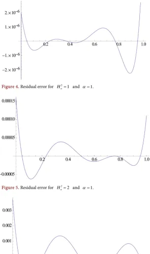
Method (LSM), Homotopy Analysis Method (HAM)and OCMI (our proposed method). The residual errors by our method are smaller than the errors obtained by Least Square Method [6] and Homotopy Analysis Method [3]. The amount of residual errors for α=1 with Ha2 =1,2,4 are depicted in Figures 4-6

respectively which infer that residual errors are quite smaller than the residual errors claimed in [6]. For 2

1

a

H = with α=4,10 the residual errors are plotted

in Figure 7 & Figure 8 which are significantly smaller as compared to the

(12)

6. Conclusion

[image:12.595.227.523.146.645.2]

In this paper, we have successfully introduced a very simple numerical method named as “orthogonal collocation-based on mixed interpolation” (OCMI). We have solved a non-linear boundary value problem governing the electrohydrodynamic

Figure 4. Residual error for 2

1

a

H = and α=1.

2

a

[image:12.595.233.518.146.314.2]

H = and α=1.

4

a

[image:12.595.229.525.528.703.2]

(13)

[image:13.595.229.524.66.440.2]

1

a

H = and α=4.

1

a

H = and α=10.

flow (EHD) in cylindrical conduit where the unknown solution is approximated by means of mixed interpolation. The approximate solutions are in excellent agreement with those of the solution given by previous researchers Mckee et al. (1997), Paullet (1999) and Ghasemi et al. (2014). The comparison of residual errors is made in Table 3 which shows the error in our method is smaller or equal to the error via Least Square Methods (LSM), Homotopy Analysis Method (HAM) for a fixed non-linearity parameter. The effect of Hartmann electric number ( 2

a

H ) is depicted in Figure 2 which shows that the conduit velocity

increases with increase in 2

a

H . On the other hand, the increasing effect of

nonlinearity parameter (α) for a fixed 2

a

H affects conduit velocity adversely.

For small values of α, conduit velocity shows rhythmic behavior but for large values of α, its behavior is adversed which is shown in Figure 3. For α1

velocity profile found to be flatten in shape, thus shown an agreement in velocity profile that claimed by Paullet [2]. The graphs of residual errors are displayed via

Figures 4-8 which infer that the amount of errors are significantly smaller than

(14)

DOI: 10.4236/jamp.2018.63050 586 Journal of Applied Mathematics and Physics of mixed interpolation we have used a fixed value of parameter k=1.5 in

correction terms. The computation of optimum value of correction parameter k

can be taken as future development in this direction.

Acknowledgements

The first author acknowledges the financial support in form of fellowship given by Dr. Harisingh Gour Vishwavidyalaya, Sagar (M.P.), India.

References

[1] Mckee, S., Watson, R., Cuminato, J.A., Caldwell, J. and Chen, M.S. (1997) Calcula-tion of Electrohydrodynamic Flow in a Circular Cylindrical Conduit. Zeitschrift für Angewandte Mathematik und Mechanik, 77, 457-465.

https://doi.org/10.1002/zamm.19970770612

[2] Paullet, J.E. (1999) On the Solution of Electrohydrodynamic Flow in a Circular Cy-lindrical Conduit. Zeitschrift für Angewandte Mathematik und Mechanik, 79, 357-360.

https://doi.org/10.1002/(SICI)1521-4001(199905)79:5<357::AID-ZAMM357>3.0.C O;2-B

[3] Mastroberardino, A. (2011) Homotopy Analysis Method Applied to Electrohydra-dynamic Flow. Communications in Nonlinear Science and Numerical Simulation, 16, 2730-2736. https://doi.org/10.1016/j.cnsns.2010.10.004

[4] Pandey, R.K., Baranwal, V.K. and Singh, C.S. (2012) Semi-Analytic Algorithms for the Electrohydrodynamic Flow Equation.Journal of Theoretical and Applied Phys-ics, 6, 45.

[5] Khan, N.A., Jamil, M., Mahmood, A. and Ara, A. (2012) Approximate Solution for the Electrohydrodynamic Flow in a Circular Cylindrical Conduit. ISRN Computa-tional Mathematics, 2012, Article ID: 341069.

[6] Ghasemi, S.E., Hatami, M., Mehdizadeh Ahangar, GH.R. and Ganji, D.D. (2014) Electrohydrodynamic Flow Analysis in a Circular Cylindrical Conduit Using Least Square Method. Journal of Electrostatics, 72, 47-52.

https://doi.org/10.1016/j.elstat.2013.11.005

[7] Saunders, R. (1985) Note on a Proposed Weighted Residual Method for Solving Nonlinear Differential Boundary Problems. Applied Mathematical Modelling, 9, 385-386. https://doi.org/10.1016/0307-904X(85)90029-0

[8] Iserles, A. (1996) A First course in the Numerical Analysis of Differential Equations, Cambridge University Press, Cambridge.

[9] de Boor, C. and Swartz, B. (1973) Collocation at Gaussian Points. SIAM Journal on Numerical Analysis, 10, 582-606. https://doi.org/10.1137/0710052

[10] Nemati, S. (2015) Numerical Solution of Volterra-Fredholm Integral Equations Us-ing Legendre Collocation Method. Journal of Computational and Applied Mathe-matics, 278, 29-36. https://doi.org/10.1016/j.cam.2014.09.030

[11] Pandey, R.K., Sharma, S. and Kumar, K. (2016) Collocation Method for Generalized Abel’s Integral Equations. Journal of Computational and Applied Mathematics, 302, 118-128. https://doi.org/10.1016/j.cam.2016.01.036

[12] Carey, G.F. and Finlayson, B.A. (1975) Orthogonal Collocation on Finite Elements, Chemical Engineering Science, 30, 587-596.

(15)

DOI: 10.4236/jamp.2018.63050 587 Journal of Applied Mathematics and Physics [13] Liu, F. and Bhatia, S.K. (1999) Computationally Efficient Solution Techniques for Adsorption Problems Involving Steep Gradients Bidisperse Particles. Computers & Chemical Engineering, 23, 933-943. https://doi.org/10.1016/S0098-1354(99)00262-8

[14] Arora, S., Dhaliwal, S.S. and Kukreja, V.K. (2005) Solution of Two Point Boundary Value Problems Using Orthogonal Collocation on Finite Elements. Applied Ma-thematics and Computation, 171, 358-370.

https://doi.org/10.1016/j.amc.2005.01.049

[15] Paterson, W.R. and Cresswell, D.L. (1971) A Simple Method for the Calculation of Effectiveness Factor. Chemical Engineering Science, 26, 605-616.

https://doi.org/10.1016/0009-2509(71)86004-9

[16] Vaferi, B., Salimi, V., Dehghan Baniani, D., Jahanmiri, A. and Khedri, S. (2012) Prediction of Transient Pressure Response in the Petroleum Reservoirs Using Ortho-gonal Collocation. Journal of Petroleum Science and Engineering, 98-99, 156-163.

https://doi.org/10.1016/j.petrol.2012.04.023

[17] Meyer, H.D., Vanthournout, J., Vanden Berghe, G. and Vanderbauwhede, A. (1990) On the Error Estimation for a New Type of Mixed Interpolation. Journal of Com-putational and Applied Mathematics, 32, 407-415.

https://doi.org/10.1016/0377-0427(90)90045-2

[18] Meyer, H.D., Vanthournout, J. and Vanden Berghe, G. (1990) On a New Type of Mixed Interpolation. Journal of Computational and Applied Mathematics, 30, 55-69.

https://doi.org/10.1016/0377-0427(90)90005-K

[19] Chakrabarti, A. and Hamsapriye (1996) Derivation of a Generalised Mixed Inter-polation Formula. Journal of Computational and Applied Mathematics, 70, 161-172.

https://doi.org/10.1016/0377-0427(96)00145-8

[20] Chakrabarti, A. and Hamsapriye (1996) Modified Quadrature Rules Based on a Ge-neralised Mixed Interpolation Formula. Journal of Computational and Applied Mathematics, 76, 239-254. https://doi.org/10.1016/S0377-0427(96)00107-0

[21] Vanden Berghe, G., Meyer, H.D. and Vanthournout, J. (1990) On a Class of Mod-ified Newton-Cotes Quadrature Formulae Based upon Mixed-Type of Interpola-tion. Journal of Computational and Applied Mathematics, 31, 331-349.