Bayesian Bin Distribution Inference and
Mutual Information
Dominik Endres and Peter Földiák
Abstract—We present an exact Bayesian treatment of a simple, yet sufficiently general probability distribution model. We con-sider piecewise-constant distributions ( ) with uniform (second-order) prior over location of discontinuity points and assigned chances. The predictive distribution and the model complexity can be determined completely from the data in a computational time that is linear in the number of degrees of freedom and quadratic in the number of possible values of . Furthermore, exact values of the expectations of entropies and their variances can be computed with polynomial effort. The expectation of the mutual information becomes thus available, too, and a strict upper bound on its variance. The resulting algorithm is particularly useful in experimental research areas where the number of available samples is severely limited (e.g., neurophysi-ology). Estimates on a simulated data set provide more accurate results than using a previously proposed method.
Index Terms—Bayesian inference, entropy, model selection, mu-tual information.
I. INTRODUCTION
T
HE small number of samples available in many areas of experimental science is a serious limitation in calculating distributions and information. For instance, such limitations are typical in the neurophysiological recording of neural activity. Computing entropies and mutual information from data of lim-ited sample size is a difficult task. A related problem is the es-timation of probability distributions and/or densities. In fact, once a good density estimate is available, one could also ex-pect the entropy estimates to be satisfactory. One of the sev-eral approaches proposed in the past is kernel-based estimation, having the advantage of being able to model virtually any den-sity, but suffering from a heavy bias, as reported by [1]. Another category consists of parametrized estimation methods, which choose some class of density function and then determine a set of parameters that best fit the data by maximizing their likeli-hood. However, maximum-likelihood approaches are prone to overfitting. A common remedy for this problem is cross vali-dation (see, e.g., [2]), which, while it appears to work in many cases, can at best be regarded as an approximation.Overfitting occurs especially when the size of the data set is not large enough compared to the number of degrees of freedom of the chosen model. Thus, as a compromise between the two aforementioned methods,mixture modelshave recently
Manuscript received August 16, 2004; revised May 12, 2005.
The authors are with the School of Psychology, University of St.Andrews, St. Andrews KY16 9JP, Scotland, U.K. (e-mail: [email protected]; [email protected]).
Communicated by P. L. Bartlett, Associate Editor for Pattern Recognition, Statistical Learning and Inference.
Digital Object Identifier 10.1109/TIT.2005.856954
attracted considerable attention (see, e.g., [3]). Here, a mixture of simple densities (Gaussians are quite common) are used to model the data. The most popular method for determining its parameters is Expectation Maximization, first described by [4], which, while having nice convergence properties, is still aiming at maximizing the likelihood. The question of how to determine the best number of model parameters therefore remains unanswered in this framework.
This answer can be given by Bayesian inference. In fact, when one is willing to accept some very natural consistency require-ments, it provides the only valid answer, as demonstrated by [5]. The difficulty lies in carrying out the necessary computations. More specifically, the integrations involved in computing the posterior densities of the model parameters are hard to tackle. To date, only fairly simple and hence not very general density models could be treated exactly. Thus, a variety of approxi-mation schemes have been devised, e.g., Laplace approxima-tion (where the true density is replaced by a Gaussian), Monte Carlo simulation, or variational Bayes (a good introduction can be found in [6]). As is always the case with approximations, they will work in some cases and fail in others. Two other note-worthy approaches to dealing with the overfitting problem are minimum message length (MML) [7] and minimum description length (MDL) [8], which are similar to Bayesian inference.
In this paper, we will present an exactly tractable model. While still simple in construction, it is sufficiently general to model any distribution (or density). The model’s complexity is fully determined by the data, too. Moreover, it also yields exact expectations of entropies and their variances. Thus, an exact expectation of the mutual information and a strict upper bound on its variance can be computed as well.
II. BAYESIANBINNING
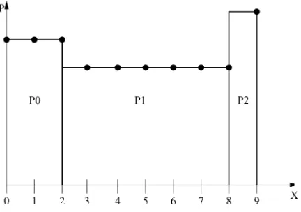
Suppose we had a discrete random variable , which could take on the values . Furthermore, assume that a notion of similarity between any two instances , of could be quantified in a meaningful way by . It is then natural to try to model the distribution of by con-tiguous, nonoverlapping bins, such that the bins cover the whole domain of . Each bin has a probability , , subject to the normalization constraint . This probability is evenly distributed among the possible values of in the bin (see Fig. 1). If a bin ends at and the previous one at , then
for all (1)
Fig. 1. An example configuration forK = 10values ofX, three bins (M = 2 interval boundaries), containing the probabilitiesP . Here,P (0) = P (1) =
P (2) = ,P (3) = 1 1 1 = P (8) = ,P (9) = P. The points indicate which values ofX belong to a bin. The algorithm iterates over all possible configurations to find the expected probability distribution and other relevant averages.
with , , and ,
i.e., the first bin starts at and the last one includes . Assume now we had a multiset
of points drawn independently from the distribution which we would like to infer. Given the model parameterized by and , the probability of the data then is given (up to a factor) by a multinomial distribution
(2)
where is the number of points in bin . One might argue that a multinomial factor should be inserted here, because the data points are not ordered. This would, however, only amount to a constant factor that cancels out when averages (posteriors, expectations of variables, etc.) are computed. It will therefore be dropped. The factors express the intention of mod-eling possible values of by the same probability. From an information-theoretic perspective, we are trying to find a sim-pler coding scheme for the data while preserving the informa-tion present in them: The message “ ” for all
would be represented by a code element of the same length . In contrast, were the absent, then the
message “ ” for each would be
represented by the same code element, i.e., an information re-duction transformation would have been applied to the data.
We now want to compute the evidence of a model with bins, i.e., . It is obtained by multiplying the likeli-hood (see (2)) with a suitable prior to yield . This density is then marginalized with respect to (w.r.t.) and , which is done by integration and summation, respectively. The summation boundaries for the have to be chosen so that each bin covers at least one possible value of . Since the bins may not overlap,
, , etc. Because the
represent probabilities, their integrations run from to
subject to the normalization constraint, which can be enforced via a Dirac function
(3)
where
(4)
and
(5)
Note that the prior is a probability density, because the are real numbers.
III. COMPUTING THEPRIOR
We shall make a noninformative prior assumption, namely, that all possible configurations of are equally likely prior to observing the data. The prior can be written as
(6)
Note that the second factor on the right-hand side (RHS) is not a probability density, because there is only a finite number of configurations for the . We now make the assumption that the probability contained in a bin is independent of the bin size, i.e.,
This is certainly not the only possible choice, but a common one: in the absence of further prior information, independence assumptions can be justified, since they maximize the prior’s entropy. Thus, (6) becomes
(7)
Since all models are to be equally likely, the prior is constant (denoted by ) w.r.t. and , and normalized
(8)
Carrying out the integrals is straightforward (see, e.g., [9]) and yields the normalization constant of a Dirichlet distribution. The value of the sums is given by
(9)
This is, of course, just the number of possibilities of distributing ordered bin boundaries across places. Due to the as-sumed independence between and , we can write
(10)
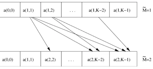
Fig. 2. After all the evidence contributionsa( ~M; ~K)have been evaluated to compute the evidence of a model withM~ intersections, they can be reused to compute thea( ~M + 1; ~K). The arrows indicate whicha( ~M; ~K)enter into the calculation for ana( ~M + 1; ~K).
and thus, the prior is
(12)
IV. COMPUTING THEEVIDENCE
To compute (3), we rewrite it as
(13)
where
(14) Given a configuration of the , the are fixed, and thus the integrals can be carried out (see, e.g., [9]) to yield
(15)
i.e., the normalization integral of a Dirichlet distribution again. Thus,
(16)
For a speedy evaluation of the sums in (13), we suggest the following iterative scheme:
let
(17)
where is the total number of data points for which (i.e., the number of points in the current bin ). Furthermore, define
(18)
where is the total number of data points for which (i.e., the number of points in the current bin ). In other words, to compute the contribution to (13) which has bin boundaries in the interval , let boundary move between position (because the previous boundaries must at least occupy the positions ) and (because bin must at least have width ). For each of these positions, multiply the factor for bin (which ranges from to ) with the contribution for bin boundaries in the interval and add.
By induction, we hence obtain
(19)
Inserting (16) into (13) and using (11) yields
(20)
This way of organizing the calculation is computationally similar to the sum–product algorithm [10], the messages being passed from one -level to the next are the , whereas within one level, a sum over the messages from the previous level (times a factor) is performed.
To compute , we need all the ,
(see Fig. 2). While we are at it, we can just as well evaluate , which does not increase the overall computation complexity. Thus, we get the evidences for models with less than intersections with little extra ef-fort. Moreover, in an implementation it is sufficient to store the in a one-dimensional array of length that is over-written in reverse order as one proceeds from to
(be-cause is no longer needed once is
computed, etc.). In pseudocode (where func-tion returns the number of observed points for which
1) Initialize ,
2) for to do
a) b) 3)
4) for to do
a) if then else
b) for downto lb do i)
ii) for to do
A) B)
c)
Step 4a) is not essential, but it saves some computational ef-fort: once the main loop 4 reaches , only needs to be calculated. The would only be necessary if the evidence for bin boundaries were to be evaluated. In a real-world implementation, it might be advisable to con-struct a lookup table for
since these quantities would otherwise be evaluated multiple times in step 4b)ii)B), as soon as .
A look at the main loop 4) shows that the computational com-plexity of this algorithm is (provided that , i.e., the number of bins is much smaller than the number of pos-sible values of ), or more generally, (because
). This is significantly faster than the naïve approach of simply trying all possible configurations, which would yield
.
V. EVALUATING THEMODELPOSTERIOR ,THE
DISTRIBUTION ,ANDITSVARIANCE
Once the evidence is known, we can proceed to determine the relative probabilities of different , themodel posterior
(21)
where is the model prior and
The sum over includes all models which we choose to include into our inference process, therefore, the conditioning on a par-ticular is marginalized. It is thus customary to refer to as “the probability of the data.” This is somewhat misleading, because is still not only conditioned on the set of we chose, but also on the general model class we consider (here: probability distributions that consist of a number of bins).
The predictive distribution of can be calculated via the evidence as well. Note that
(22)
i.e., the joint predictive probability of is the ex-pectation of the product of their probabilities given and . Thus, if we want the value of the predictive distribution of at a particular , we can simply add this to the multiset . Call this extended multiset , then
(23)
The choice of will usually be noninformative (e.g., uni-form), unless we have reasons to prefer certain models over others.
Likewise, to obtain the variance, add twice: . Then
(24)
VI. INFERRINGPROBABILITYDENSITIES
The algorithm can also be used to estimate probability densi-ties. To do so, replace all occurrences of with , where is the interval between and . This yields a dis-cretized approximation to the density. The discretization is just another model parameter which can be determined from the data
(25)
where runs over all possible values of which we choose to include. is computed in the same fashion as in (21) for a given , except that the data are now assumed to be continuous, hence, the probability turns into a density.
The dependence of on is through (see (3)): if one tries to find a suitable discretization of the interval
, then .
VII. MODELSELECTIONVERSUSMODELAVERAGING
Once is determined, we could use it to select an . However, making this decision involves “contriving” in-formation, namely, nats. Thus, unless one is forced to do so, one should refrain from it and rather average any predictions over all possible . Since , com-puting such an average has a computational cost of . If the structure of the data allows for it, it is possible to reduce this cost by finding a range of that does not increase linearly with , without a high risk of not including a model even though it provides a good description of the data. In analogy to the sig-nificance levels of orthodox statistics, we shall call this risk . If the posterior of is unimodal (which it has been in most observed cases, see, e.g., Seection IX), we can then choose the smallest interval of s around the maximum of such that
(26)
VIII. COMPUTING THEENTROPY AND ITSVARIANCE
To evaluate the entropy of the distribution , we first compute the entropy of (1)
(27)
where is the natural logarithm. This expression must now be averaged over the posterior distributions of
and possibly to obtain the expectation of . In-stead of carrying this out for (27) as a whole, it is easier to do it term-by-term, i.e., we need to calculate the expectations of
and . Generally speaking, if
we want to compute the average of any quantity that is a func-tion of the probability in a bin for a given , we can proceed in the following fashion: call this function . Its expecta-tion w.r.t. the is then
(28) where, by virtue of (14) and (15)
(29)
because is a constant, otherwise it would have to be included in the integrations. Note that, as far as the counts in the
bins are concerned, depends only
on (and possibly , the total number of data points). This can be verified by integrating the numerator of (28) over all ,
. Therefore,
(30)
When (29) is inserted here, it becomes apparent that this ex-pectation has the same form as (13) after inserting (16).
Com-bined with the fact that depends only
on , this means that the above described iterative computa-tion scheme ((17) and (18)) can be employed for its evaluacomputa-tion. All one needs to do is to substitute
i.e., (18) is replaced by
(31)
where and . The for
are the same as before. Note that (31) can also be used if depends not only on , but also on the boundaries of bin (i.e., and ). Generally speaking, (31) can be employed whenever the expectation of a function (given and ) is to be evaluated, if this function depends only on the parameters of one bin.
For fixed , some of these expectations have been com-puted before in [9].
A. Computing
Using (1) and defining , we obtain
(32)
To compute the integrals, note that
(33)
which is
(34)
where is the beta function (see, e.g., [11] for details on its derivatives and other properties), and
(35)
is the difference between the partial sums of the harmonic series with upper limits and . The first part of (34) is the normal-ization integral of the density of the . Hence, their entropy for fixed is given by (34) divided by (15)
(36) which is a rational number. In other words, entropy changes in rational increments as we observe new data points.
Thus,
B. Computing
Here
(38)
and by using the same identities as above
(39)
C. Computing the Variance
To compute the variance, we need the square of the entropy
(40)
Hence, we need to evaluate the expectations of 1) . See Section VIII-D.
2) . See Section VIII-E.
3) . Can be evaluated along the same lines as (39) and yields
(41)
4) . Follows from (15) by
replacing with , with , and yields
(42)
5) . Can be evaluated along the
same lines as (37) and yields
(43)
6) . Can be evaluated along
the same lines as (37) and yields
(44) In an actual implementation, steps 1), 3), and 5) can be computed in one run, because they contain only terms that refer to the bin . Likewise, the remaining three steps can be evaluated together. However, since they depend on the parameters of two distinct bins, the iteration over the bin configuration has to be adapted: assume . This is no restriction, since and can always be exchanged to satisfy this constraint. As we will show later, the quanti-ties of interest can be expressed as products of expectations . The itera-tion rule (18) then is
(45)
and
(46)
D. Computing
Since
(47)
we can use the same method of calculation as above. Thus, we obtain
(48)
where
(49)
E. Computing
To compute this expectation, we need to evaluate
(50)
and then divide it by a normalization constant. The integrals in the last expression can be rewritten, using beta functions, to yield
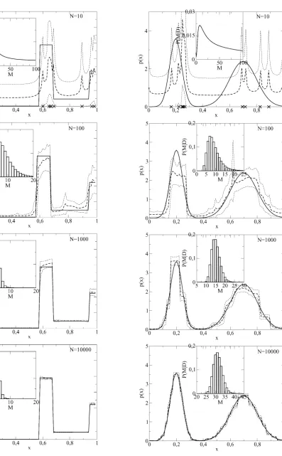
Fig. 3. From top to bottom: densities and posteriors for 10,100,1000 and 10000 data points. Expected probability density (thick dashed line) plus/minus one standard deviation (thin dashed lines), compared to the true density (thick solid line). Insets: posterior distribution ofM, the number of intersections. The arrows indicate the true value ofM = 5. TheX’s on the abscissa of the graph for 10 data points mark the data points.
Fig. 4. From top to bottom: densities and posteriors for 10,100,1000 and 10000 data points. Expected probability density (thick dashed line) plus/minus one standard deviation (thin dashed lines), compared to the true density (thick solid line). Insets: posterior distribution ofM, the number of intersections. The
[image:7.594.64.272.66.686.2]where and is the part that does not depend upon and and, thus, is not affected by the dif-ferentiation
(52)
We then obtain
(53)
The desired expectation can thus be computed in two runs of the iteration: first, let
(54)
(55)
and divide the result by .
Second, let
(56) (57)
and multiply the result with .
IX. EXAMPLES
Fig. 3 shows examples of the predictive density and its variance, compared to the density from which the data points were drawn ( , , data point abscissas were rounded to the next lower discretization point), as well as the model posteriors . The prior was chosen uniform over the maximum range of , here . Inference was conducted with (see (26)).1Note that
the curves that represent the expected density plus/minus one standard deviation are not densities any more. The data were produced by first drawing uniform random numbers with the generator sran2() from [12], those were then transformed by the inverse cumulative density (a method also described in [12]) to be distributed according to the desired density. For very small data sets, only the largest structures of the distribution can vaguely be seen (such as the valley between and ). Furthermore, the density peaks at each data point (at , two points were observed very close to each other). One might therefore imagine the process by which the density comes about as similar to kernel-based density estimates. It does, however, differ from a kernel-based procedure insofar as that the number of degrees of freedom does not necessarily grow with the data set, but is determined by the data’s structure. The model poste-rior is very broad, reflecting the large remaining uncertainties due to the small data set. Models with were included in the predictions.
With 100 data points, more structures begin to emerge (e.g., the high plateau between and ), and the variance de-creases, as one would expect. The model posterior exhibits a
1On a 2.6-GHz Pentium 4 system running SuSE Linux 8.2, computing the
[image:8.594.313.542.63.221.2]ev-idence took0.26 s (without initializations). The algorithm was implemented in C++ and compiled with the GnU compiler.
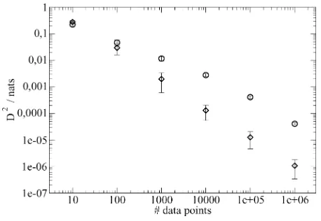
Fig. 5. D between true and expected density as a function of the number of data points. The error bars were obtained from averaging over 100 different data sets drawn from the same density. Diamonds: five-bin density (see Fig. 3), circles: mixture of two Gaussians (see Fig. 4). For details, see text.
much narrower maximum, here the included models were those
with .
At 1000 data points, most structures of the original density are modeled, except for the peak at , and the variance is yet smaller. The algorithm is now fairly certain about the cor-rect number of intersections, , with a maximum at , indicating that the algorithm has not yet discovered the peak at . Moreover, due to this restriction on the degrees of freedom, the predicted density no longer looks like a kernel-based estimate.
The peak at rises out of the background at 10 000 data points, which is also reflected in the fact that the maximum of the model posterior is now at five intersections. All structures of the distribution are now faithfully modeled.
Fig. 4 depicts density estimates from a mixture of two Gaussians. Even though these densities cannot—strictly speaking—be modeled any more by a finite number of bins, the method still produces fairly good estimates of the discretized ( ) densities. Observe how the maximum of the posterior shifts toward higher values as the number of data points grows. The algorithm thus picks a range of which, depending on the amount of available information, is best suited for explaining the underlying structure of the data.
For a more quantitative representation of the relationship between and the “closeness” of expected and true densities, Fig. 5 shows the value of a special instance of the Jensen– Shannon divergence
(58)
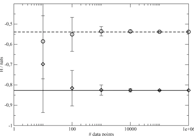
Fig. 6. Expected entropy and expected standard deviation as a function of the number of data points. Both expectations were computed for one data set at a time, then averaged over 100 data sets. The lines represent the true entropies. Diamonds, solid line: five-bin density (see Fig. 3). Circles, dashed line: mixture of two Gaussians (see Fig. 4).
Moreover, in the case of the bin density, the gain is inversely proportional to the number of data points. In other words, the decision as to which density the sample was drawn from be-comes twice as hard when is doubled.
In Fig. 6, the expected entropies are plotted as a function of the number of data points. Error bars represent expected standard deviation. Both expectations were computed individu-ally for each data set and then averaged over 100 runs. In every case, the true entropy is well within the error bars. For , the expected entropy is fairly close to its true value, thus elimi-nating the need for finite-size corrections. Note that the standard deviation of the entropy is plotted,not the empirical standard deviation of its expectation, i.e., the error bars serve as an indi-cation of the remaining uncertainty in the entropy, which goes to as increases. This is due to the fact that entropy is treated here as a deterministic quantity, not as a random variable (be-cause samples are drawn from some fixed, albeit possibly un-known, density). To illustrate this point further, look at Fig. 7: For small data sets, the empirical standard deviation of the ex-pectation of the entropy is somewhat smaller than the standard deviation of the entropy. When evaluating experimental results, using the former instead of the latter would thus possibly mis-lead one to believe in a higher accuracy of the results than can be justified by the data, a danger that is especially preeminent when using methods such as cross validation in place of exact calculations.
A. The Limit
Assume we tried to find the best discretization of the data via (25). If there is no lower limit on (other than ) given by the problem we are studying (e.g., accuracy limits of the equipment used to record the data), then we might wonder how the discretization posterior behaves as
or, conversely, as . In this case, given that stays finite, the data’s probability density will diverge whenever a data point is located in an infinitesimally small bin. However,
Fig. 7. Expected standard deviation of the entropy (diamonds: five-bin density, circles: mixture of two Gaussians) 61 standard deviation and empirical standard deviation (triangle up: five-bin density, triangle down: mixture of two Gaussians) of the expectation of the entropy as functions of the number of data points. Error bars and empirical standard deviations are averages over 100 data sets.
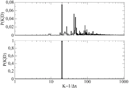
since the number of possible bin configurations also diverges, it is not clear whether stays finite or not. We will not try to give an analytic answer to this question here. Instead, look at Fig. 8, which shows the discretization posterior
(normalized on the interval , uniform prior over ) for two data sets with (top) and
[image:9.594.310.544.328.481.2]Fig. 8. Discretization posteriorP (KjD)for a data set containing 100 (top) and 1000 (bottom) data points. In the latter case, the MAP choiceK = 20can certainly be justified, for 100 data points, additional information is necessary before aKcan be picked.
evenly spread, and additional prior information is required if a choice is to be made with reasonable certainty.
There is numerical evidence which suggests that ac-tually approaches a (nonzero) constant as (not visible in the graphs, because appears to be
( ) and ( ) times smaller than the
maximum). This implies that the bulk of the probability is con-centrated around . We would, however, argue that since the presented algorithm is not useful in this limit (because it has a computational complexity ), one will always have to choose a reasonable upper bound for , determined by the available computation time, or by the accuracy of the data. Once this bound is set, a can be determined if enough data are avail-able. Alternatively, a uniform prior over (i.e., in ) could also be motivated, which would allow for a cutoff at a moderately large .
Another quantity of interest is the predictive density . Its behavior is depicted in Fig. 9, bottom, for and four different, small data sets. Other values of give qualitatively similar results. As ,
appears to diverge logarithmically with if evaluated at a data point, and to approach a constant (for given , , and ) otherwise. This suggests that the divergence is such that the probability contained in the vicinity of a data point approaches a constant as well. Numerical evidence for this hypothesis is shown in Fig. 9, top. In other words, in the limit , the predictive distribution seems to have a -peak at each data point. This behavior, which was conjectured by one of the reviewers, is reminiscent of that of a Dirichlet process [14].
X. EXTENSION TOMULTIPLECLASSES
Assume each data point was labeled, the label being . In other words, each is drawn from one of classes. We will now extend the algorithm so as to infer the joint distribution (or density) , where
.
[image:10.594.52.276.65.218.2]Instead of probabilities, we now have . is the probability mass between and in class , i.e., we assume that the bins are located at the same places across
Fig. 9. Bottom: Predictive densities p(xjD; M = 10)as a function of
K = . Circles:p(xjD; M = 10)at the location (0.4) of a data point, squares: p(xjD; M = 10) between data points. The lines denote data sets withN = 1 (solid),2(dashed),4(dotted), and8(dash-dotted). The predictive density appears to diverge logarithmically withKat the location of a data point, and remains finite elsewhere. Top: Predictive probability
P (x 2 [0:395; 0:405]jD; M = 10)in the vicinity of a data point as a function ofK. This probability seems to asymptote at a constant value forK ! 1, which indicates that the predictive density has a-peak at each data point.
classes. This might seem like a rather arbitrary restriction. We shall, however, impose it for two reasons.
1) The algorithm for iterating over the bin configurations keeps a simple form, similar to (17) and (18).
2) If we allowed different sets of for the classes, com-puting marginal distributions and entropies would become exceedingly difficult. While possible in principle, it would involve confluent hypergeometric functions and a signifi-cantly increased computational cost.
Let be the number of data points in class and bin , and . The likelihood (2) now becomes
(59)
Thus, following the same reasoning as above, the iteration rules now are
(60)
where is the total number of data points in class for which
and . Furthermore
(61)
where is the total number of data points in class for
which , and .
We can now evaluate the expected joint distribution and its variance at any , using (23) and (24) as before. To compute the marginal distribution, note that
(62)
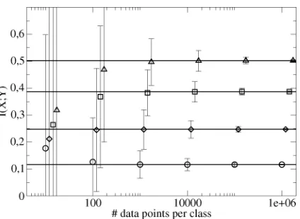
Fig. 10. Expected mutual informations and upper bounds on the standard deviations, computed via (65) for different data set sizes. The lines indicates the true mutual information. Circles: I(X; Y ) = 0.1173 nat, diamonds:
I(X; Y ) =0.2472 nat, squares:I(X; Y ) =0.3870 nat, triangles:I(X; Y ) = 0.502 nat. Mutual informations were evaluated at 10, 100, 1000, 10 000, 100 000 and 1 000 000 data points; symbols in the plot are shifted to the right to disentangle the error bars.
XI. COMPUTING THEMUTUALINFORMATION AND ANUPPER
BOUND ONITSVARIANCE
The mutual information between class label and is given by (63) which has to be averaged over the posterior distribution of the
model parameters . This can be
accom-plished term-by-term, as described above, yielding the exact expectation of the mutual information under the posterior. The evaluation of its variance is somewhat more difficult, due
to the mixed terms , ,
and . For the time being, we shall thus be content with an upper bound. Using the identity
(64)
we obtain
(65) All terms on the RHS can be computed as above.
Fig. 10 shows the results of some test runs on artificial data. Points were drawn from two classes with equal probability. Within each class, a three-bin distribution was used to generate the data. The probabilities in the bins were varied to create four different values of the mutual information. Before inferring the mutual information from the data, we first determined the best discretization step size (via the maximum of (25); this ap-proach seems to yield good results for the mutual information, even when the discretization posterior probability is not very concentrated at one ). The depicted values are individual averages over 100 data sets. In all cases, its true value lies well within the error bars. However, especially for small sample sizes, they seem rather too large—an indication that the upper bound given by (65) needs future refinement. However, observe that the expectation of is close to its true value from 100 data points per class onwards. This is an indication that the algorithm performs well for moderate sample sizes, without the need for finite-size corrections.
XII. SPARSEPRIORS
The uniform prior (8) is a reasonable choice in circumstances where no information is available about the dataa prioriother than their range. Should more be known, it is sensible to incor-porate this knowledge into the algorithm so as to speed up the in-ference process (i.e., allow for better predictions from small data sets). In the following, we will examine symmetric Dirichlet priors of the form
(66)
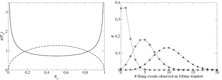
where to avoid divergence of the normalization constant. Fig. 11, left, shows the resulting priors for (two bins, thus, is beta-distributed) and two different values of . The symmetry arises from the condition . The curve for (solid line) exhibits the typical behavior expected for : Extreme values are favored because
as approaches or . Thus, this range of will generally favor distributions where few bins contain most of the proba-bility mass, i.e.,sparsedistributions. Conversely, the curve for (dashed line) indicates the general behavior expected for : the prior now promotes moderate values of . There-fore, the probability mass will tend to be more evenly distributed (dense distributions). For , the uniform prior is recovered. In typical single-cell neurophysiological experiments, sparse distributions are frequently encountered. Consider the following setup: a mammal is presented with a visual stimulus and the firing events produced by one of its visual cortex neurons are recorded in some suitably chosen time window. Assume that the temporal resolution of the recording equipment was 1 ms and the window width 100 ms. A simple model for the firing be-havior is the Poisson process, i.e., a constant probability of observing an event at any given time within the window. The ex-pected distribution of the number of observed events is then gov-erned by a binominal distribution. Fig. 11, right, depicts three such distributions for small to medium values of . While up to 100 observed events in the window are possible in prin-ciple, those values are extremely unlikely. Hence, a sparseness promoting prior can be expected to speed up convergence when such (or similar) distributions are to be inferred from data.
The algorithm can be generalized to include . Setting , (10) now becomes
(67)
Likewise, (16) is to be replaced by
(68)
This expression is again a product of the counts observed in dif-ferent bins and the bin width, times a factor which only depends on the total number of bins and data points. Hence, the same sum–product decomposition scheme as before can be used, with (17) and (18) now being
Fig. 11. Left: Prior forM = 1and two choices of: = 0:5(solid line) and = 1:5(dashed line). The first prior favors extreme values ofP , i.e., sparse distributions, the second one promotes moderate values ofP (dense distributions). Right: Binominal distributions are simple models for the distributions of spike counts observed in a fixed-time window. The curves were computed forP = 0:01(circles),P = 0:05(squares), andP = 0:1(triangles). Values are plotted only up to a spike count of 20, even though a maximum of 100 would have been possible. However, the probabilities for counts greater than 20 are virtually zero. Thus, most possible values are virtually never assumed, i.e., the distributions are sparse.
(70)
This allows for the computation of evidences and expected probabilities and their variances. To compute entropies and mu-tual informations and their variances, the relevant averages have to be adapted as well: after some tedious but straightforward cal-culus, we find that (37) has to be substituted by
(71)
where is the digamma function and
(72)
(73)
While the term in the square brackets could be written as the dif-ference between two digamma functions, decomposing it into a part that depends both on the prior and on the data and a part that depends only on the prior (i.e., and ) allows for a pre-computation of the latter. Equation (39) becomes
(74) Likewise, for (48)
(75)
and finally, we obtain for (54)
(76)
(77)
then divide the results of the averaging by , and for (56)
(78) (79)
and multiply the averages by .
The question which remains is how to choose . Since the sparseness of a distribution will usually not be knowna priori, a feasible way is to treat it as another hyperparameter to be in-ferred from the data. However, integrating over is computa-tionally rather expensive. Instead, we tried a maximuma pos-terioriapproach (the posterior density of was unimodal in all observed cases), which seems to work quite well.
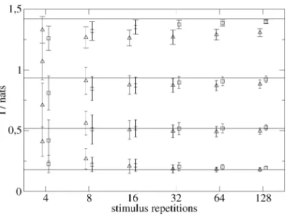
To compare the performance of the modified algorithm on sparse distributions with a method proposed in [15], we chose a way similar to that used in that paper: for a set of eight “stimuli,” distributions of responses, i.e., “mean firing rates,” were gen-erated by drawing random variables from binominal distribu-tions with different values of . These firing probabilities were functions of the stimulus label . The expected mutual information between and the responses were subsequently computed.
Fig. 12. Results of the modified algorithm on artificially created “neural responses” to eight “stimuli” (squares), compared with the method described in [15] (triangles). Mutual informations were evaluated at 4, 8, 16, 32, 64, and 128 stimulus repetitions for both methods, the symbols in the plot are shifted slightly to the left and to the right to disentangle the error bars. The response distributions were binominals with differentP ’s. Error bars are61standard deviations, obtained from averaging over 100 data sets. The lines represent the true mutual informations.
response) pairs with a fixed number of stimulus repetitions (be-tween 4 and 128). The error bars are the estimated standard devi-ations of the mutual information, not the standard errors. Fig. 12 shows the results. The squares are the expectations computed by our algorithm. The triangles depict the mutual information es-timates computed from the observed frequencies corrected by the first-order bias term reported in [15]. Those frequencies, as described in [15], were obtained by a simple discretization of the response space. Even for a rather small number of stimulus repetitions, the algorithm performs quite well, getting better as the size of the data set increases. In the great majority of cases, it appears to be more accurate than the finite-size corrected es-timates, even though the latter yield reasonable results as well if the number of stimulus repetitions is greater than the number of stimuli. Moreover, the small error bars indicate that reliable results can be expected with our method even if only a single data set is available.
XIII. CONCLUSION
The presented algorithm computes exact evidences and relevant expectations of probability distributions/densities with polynomial computational effort. This is a significant improvement over the naïve approach, which requires an expo-nential growth of the number of operations with the degrees of freedom. It is also able to find the optimal number of degrees of freedom necessary to explain the data, without the danger of overfitting. Furthermore, the expectations of entropies and mutual information have been shown to be close to their true values for relatively small sample sizes. In the past, a variety of methods for dealing with systematic errors due to small sample sizes have been proposed, such as stimulus shuffling in [16] or regularization of neural responses by convolving them with Gaussian kernels. While these approaches work to some degree, they lack the sound theoretical foundation of exact Bayesian treatments.
In [15], finite size corrections are given based on the number of effective bins, i.e., the number of bins necessary to explain
[image:13.594.62.271.62.220.2]the data. There, it is also demonstrated that this leads to in-formation estimates which converge much more rapidly to the true value than the other techniques mentioned (shuffling and convolving). However, as authors of [15] themselves admit, their method of choosing the number of effective bins is only “Bayesian-like.” Furthermore, their initial regularization ap-plied to the data—choosing a number of bins that is equal to the number of stimuli and then setting the bin boundaries so that all bins contain the same number of data points, a procedure also used by [17]–is debatable (it should, however, be pointed out that this equiprobable binning procedure is not an essen-tial ingredient for the successful application of the finite-size corrections of [15]. It has recently been demonstrated [18] that, given a decent amount of data is available, the methods of [15] can be used to yield reasonably unbiased estimates for ). On the one hand, one might argue that the posterior of is still broad when the data set is small (see Fig. 3, graphs for 10 and 100 data points), so choosing the wrong number of bins will do little damage. On the other hand, the bin boundaries must certainly not be chosen in such a way that all bins contain the same number of points. Doing so will destroy the structure present in the data. Consider e.g., Fig. 3, graph for 1000 data points: there are many more data points in the interval than there are between , which reflects a feature of the distribution from which the data were drawn and should thus be modeled by any good density estimation technique. This will, however, not be the case if the boundaries are chosen as proposed: there would be a boundary somewhere at instead of , and the step at this point would be replaced by a considerably smaller one at , thus misrepresenting the underlying distribution. In other words, that procedure would not even converge to the correct distribution as the data set size grows larger, unless the number of bins was allowed to grow with the data set. But that might introduce unnecessary degrees of freedom. Consequently, mutual information estimates calculated from those estimated distributions must be interpreted with great care.
We believe to have shown that those drawbacks can be over-come by a Bayesian treatment, which also seems to show im-proved performance over finite-size corrections. Thus, the algo-rithm should be useful in several areas of research where large data sets are hard to come by, such as neuroscience.
Another interesting Bayesian approach to removing finite-size effects in entropy estimation is the Nemenman–Shafee– Bialek (NSB) method [19]. It exploits the fact that the typical distributions under the symmetric Dirichlet prior (66) have very similar entropies, with a variance that vanishes as grows large. This observation is then employed to construct a prior which is (almost) uniform in the entropy. The resulting estimator is demonstrated to work very well even for relatively small data sets.
It was proven in [20] that uniformly (over all possible dis-tributions) consistent entropy estimators can be constructed for distributions comprised of any number of bins , even if
. The above presented results (Fig. 6) suggest that the ex-pected entropies computed with our algorithm are asymptoti-cally unbiased and consistent. Furthermore, the true entropy was usually found within the expected standard deviation. It remains to be determined how the algorithm performs if .
Since the upper bound (65) on the variance of the mutual information is rather large for small sample sizes, it might be interesting to invest some more work into computing the exact variance of the mutual information. This, however, turns out to be difficult.
ACKNOWLEDGMENT
The authors would like to thank Johannes Schindelin for many stimulating discussions. Furthermore, they are also grateful to the anonymous reviewers for their helpful sugges-tions and references.
REFERENCES
[1] M. Rosenblatt, “Remarks on some nonparametric estimates of a density function,”Ann. Math. Statist., vol. 27, pp. 832–837, 1956.
[2] M. Stone, “Cross-validatory choice and assessment of statistical predic-tions,”J. Roy. Statist. Soc., Ser. B, vol. 36, no. 1, pp. 111–147, 1974. [3] N. Ueda, R. Nakano, Z. Ghahramani, and G. E. Hinton, “SMEM
algo-rithm for mixture models,”Neur. Comput., vol. 12, no. 9, pp. 2109–2128, 2000.
[4] A. Dempster, N. Laird, and D. Rubin, “Maximum likelihood for incom-plete data via the EM algorithm,”J. Roy. Statist. Soc., Ser, B, vol. 39, no. 1, pp. 1–38, 1977.
[5] R. Cox, “Probability, frequency and reasonable expectation,”Amer. J. Phys., vol. 14, no. 1, pp. 1–13, 1946.
[6] M. Jordan, Z. Ghahramani, T. Jaakkola, and L. Saul, “An introduction to variational methods for graphical models,”Mach. Learn., vol. 37, no. 2, pp. 183–233, 1999.
[7] C. Wallace and D. Boulton, “An information measure for classification,”
Comput. J., vol. 11, pp. 185–194, 1968.
[8] J. Rissanen, “Modeling by shortest data description,”Automatica, vol. 14, pp. 465–471, 1978.
[9] M. Hutter, “Distribution of mutual information,” inAdvances in Neural Information Processing Systems. Cambridge, MA: MIT Press, 2002, vol. 14, pp. 339–406.
[10] F. Kschischang, B. Frey, and H.-A. Loeliger, “Factor graphs and the sum-product algorithm,”IEEE Trans. Inf. Theory, vol. 47, no. 2, pp. 498–519, Feb. 2001.
[11] P. Davis, “Gamma function and related functions,” in Handbook of Mathematical Functions, M. Abramowitz and I. Stegun, Eds. New York: Dover, 1972.
[12] W. Press, B. Flannery, S. Teukolsky, and W. Vetterling, Numerical Recipes in C: The Art of Scientific Computing. New York: Cambridge Univ. Press, 1986.
[13] D. Endres and J. Schindelin, “A new metric for probability distribu-tions,”IEEE Trans. Inf. Theory, vol. 49, no. 7, pp. 1858–1860, Jul. 2003. [14] T. S. Ferguson, “Prior distributions on spaces of probability measures,”
Ann. Statist., vol. 2, no. 4, pp. 615–629, 1974.
[15] S. Panzeri and A. Treves, “Analytical estimates of limited sampling bi-ases in different information measures,”Network: Comp. Neur. Syst., vol. 7, pp. 87–107, 1996.
[16] L. Optican, T. Gawne, B. Richmond, and P. Joseph, “Unbiased measures of transmitted information and channel capacity from multivariate neu-ronal data,”Biol. Cybern., vol. 65, pp. 305–310, 1991.
[17] E. Rolls, H. Critchley, and A. Treves, “The representation of olfactory information in the primate orbitofrontal cortex,”J. Neurophys., vol. 75, pp. 1982–1996, 1995.
[18] E. Arabzadeh, S. Panzeri, and M. Diamond, “Whisker vibration infor-mation carried by rat barrel cortex neurons,”J. Neurosci., vol. 24, no. 26, pp. 6011–6020, 2004.
[19] I. Nemenman, W. Bialek, and R. van Steveninck, “Entropy and infor-mation in neural spike trains: Progress on the sampling problem,”Phys. Rev. E, vol. 69, no. 5, 2004.