Assessment and weighting of meteorological ensemble forecast members based on supervised machine learning with application to runoff simulations and flood warning

1 2 3 4 5 6 7 8 9 10 11 12 13 14 15 16 17 18 19 20 21 22 23 24 25 26 27 28 29 30 31 32 33 34 35 36 37 38 39 40 41 42 43 44 45 46 47 48 49 50 51 52 53 54 55 56 57 58 59 60 61

Assessment and weighting of meteorological ensemble forecast members

based on supervised machine learning with application to runoff

simulations and flood warning

Kristina Doycheva, [email protected] Ruhr-University Bochum, Germany Gordon Horn, [email protected]

Ruhr-University Bochum, Germany

Christian Koch, [email protected] University of Nottingham, United Kingdom Andreas Schumann, [email protected]

Ruhr-University Bochum, Germany Markus König, [email protected]

Ruhr-University Bochum, Germany

Abstract

Numerical weather forecasts, such as meteorological forecasts of precipitation, are inherently

uncertain. These uncertainties depend on model physics as well as initial and boundary

conditions. Since precipitation forecasts form the input into hydrological models, the

uncertainties of the precipitation forecasts result in uncertainties of flood forecasts. In order to

consider these uncertainties, ensemble prediction systems are applied. These systems consist

of several members simulated by different models or using a single model under varying

initial and boundary conditions. However, a too wide uncertainty range obtained as a result of

taking into account members with poor prediction skills may lead to underestimation or

exaggeration of the risk of hazardous events. Therefore, the uncertainty range of model-based

flood forecasts derived from the meteorological ensembles has to be restricted.

In this paper, a methodology towards improving flood forecasts by weighting ensemble

members according to their skills is presented. The skill of each ensemble member is

evaluated by comparing the results of forecasts corresponding to this member with observed

values in the past. Since numerous forecasts are required in order to reliably evaluate the

skill, the evaluation procedure is time-consuming and tedious. Moreover, the evaluation is

highly subjective, because an expert who performs it makes his decision based on his implicit

knowledge.

Therefore, approaches for the automated evaluation of such forecasts are required. Here, we

present a semi-automated approach for the assessment of precipitation forecast ensemble

*Manuscript

1 2 3 4 5 6 7 8 9 10 11 12 13 14 15 16 17 18 19 20 21 22 23 24 25 26 27 28 29 30 31 32 33 34 35 36 37 38 39 40 41 42 43 44 45 46 47 48 49 50 51 52 53 54 55 56 57 58 59 60 61

members. The approach is based on supervised machine learning and was tested on ensemble

precipitation forecasts for the area of the Mulde river basin in Germany. Based on the

evaluation results of the specific ensemble members, weights corresponding to their forecast

skill were calculated. These weights were then successfully used to reduce the uncertainties

within rainfall-runoff simulations and flood risk predictions.

Keywords: precipitation forecast, supervised machine learning, pattern recognition,

uncertainty

1. INTRODUCTION

Flood forecasts in small and medium-sized river basins are usually based on precipitation

forecasts. These forecasts are derived by deterministic numerical weather models. As a result,

the flood forecasts depend on model physics, initial and boundary conditions. Since the

meteorological and hydrological processes are very complex, these forecasts are associated

with a high level of uncertainty.

Conventional precipitation forecasts lead to unsatisfactory results because of these

uncertainties (Schüttemeyer and Simmer 2011). With the aim to limit the range of the

uncertainties, ensemble forecasting methods and ensemble prediction systems (EPS) are

being applied more and more often (Schumann et al. 2011). The ensemble forecasting

process includes several simulation runs using one or multiple models with perturbed initial

conditions, varied parameter sets, or different model physics (Cloke & Pappenberger 2009).

The individual combinations of these models and conditions, which are used for the multiple

simulations, are referred to as ensemble members. Hence, an ensemble forecast predicts a

vector of values for one specific point in time at one and the same location. This vector of

values should ideally represent the range of possible developments in the near future.

In general, it is assumed that the probability of an ensemble member leading to a reliable

forecast is the same among all ensemble members and the diversity of the members

compensates for errors, either due to lack of comprehensive initial data, accuracy and quality

of the initial data, or due to model resolutions that do not sufficiently capture all features of

the observed event (WPC 2006). However, in some cases the inclusion of less skillful

members degrades the quality of the ensemble prediction. This could lead to underestimation

1 2 3 4 5 6 7 8 9 10 11 12 13 14 15 16 17 18 19 20 21 22 23 24 25 26 27 28 29 30 31 32 33 34 35 36 37 38 39 40 41 42 43 44 45 46 47 48 49 50 51 52 53 54 55 56 57 58 59 60 61

possibility of a flood due to considering too many “poor” ensemble members could result in a

missing warning. Vice versa, overestimating the probability of a flood to occur would lead to

many false alarms, which may encourage people to ignore warnings in the future (Dietrich et

al. 2009).

In order to overcome these limitations, this paper suggest to improve the capability of

ensemble prediction systems by introducing weights to the members based on their forecast

skill. In meteorological context, the term forecast skill refers to the accuracy of a prediction

to an observed event (AMS 2000). To apply a probabilistic assessment of meteorological

ensemble members, their performance to describe an observed event in the past can be used.

By post-processing such events, forecasters can assign smaller weights to members with a

poor prediction quality (less skilled members) or completely exclude such members from the

ensemble to improve the overall quality of the forecast.

Some statistical methods to determine the performance of the individual members have been

presented. However, further research into improved methods is still needed. Recently,

examples have been presented that demonstrate unexpected skill with common deterministic

verification metrics, such as the Brier skill score or relative operating characteristics (Hamill

& Juras 2006), For this reason, methods which are not purely based on statistical measures

need to be investigated. Instead of statistical measures, the knowledge and experience of

hydrology experts could be employed in order to evaluate the performance of different

ensemble members. Usually, the assessment procedure is completely manual and

time-consuming, because numerous forecasts including thousands of ensemble members need to

be considered.

Yet, the limitations of the manual assessment procedure can be compensated by utilizing

automated approaches for forecast assessment. However, the knowledge of these experts is a

so-called tacit knowledge. Tacit knowledge is difficult to transfer to another person by means

of writing it down or verbalizing it. As a result, the knowledge of the experts cannot easily or

directly be transferred to a software system. Consequently, a kind of an automated training

and learning system that maps the expert’s knowledge onto a software system is required in

order to accelerate the assessment and weighting procedure.

In this paper we present an approach to assess precipitation forecasts based on supervised

machine learning and use higher quality forecasts to reduce the uncertainty of flood risk

predictions. The paper is structured as follows. Section 2 presents existing relevant and

1 2 3 4 5 6 7 8 9 10 11 12 13 14 15 16 17 18 19 20 21 22 23 24 25 26 27 28 29 30 31 32 33 34 35 36 37 38 39 40 41 42 43 44 45 46 47 48 49 50 51 52 53 54 55 56 57 58 59 60 61

while a case study is described in section 4. In particular, the observed area, the ensemble

prediction system used to forecast precipitation, and the hydrological runoff simulation model

are presented. The paper concludes with a summary and an outlook on future research.

2. RELATED WORK

Several assessment approaches, mostly based on statistical measurements, have already been

proposed. Garaud and Mallet (2011) measured the quality of uncertainty estimation, and the

reliability and the resolution of an ensemble using the Brier score, or scores derived from the

rank histogram or the reliability diagram. Eckel and Walters (1998) used the verification rank

histogram to interpret and adjust an ensemble probabilistic quantitative precipitation

forecasts. Krishnamurti (1999) used a weighted multi model ensemble to produce one

averaged forecast. The weights were obtained by using multiple regressions between the

model forecast and the observed data during a training period. However, Hamill and

Swinbank (2014) addressed the need of reducing systematic errors in numerical weather

predictions. According to their work, statistical post-processing methods may be applied for

this purpose, but continuous research into improved methods is still needed.

Hamill and Juras (2006) also presented examples that demonstrate unexpected skill with

common deterministic verification metrics, such as the Brier skill score or relative operating

characteristic. Raftery et al. (2005) used Bayesian model averaging for statistical post

processing of meteorological forecasts, which was later extended specifically for probabilistic

quantitative precipitation forecasts by Sloughter et al. (2007). Beside Bayesian model

averaging, Casanova and Ahrens (2009) applied a simpler skill-based weighting method,

using the normalized inverses of the mean-square errors of the forecast in a training period as

weights. Gneiting et al. (2005) introduced the ensemble model output statistic. This

post-processing technique also uses multiple linear regression and can be applied to any ensemble

system and forecast variable, including precipitation, with some modification. Weusthoff et

al. (2011) also tried to classify precipitation forecasts into good and bad members. Although

they also used a spatial approach, they applied an optical flow technique (Keil and Craig

2009) for their classification process.

Brochero et al. (2011) applied backward greedy selection to assess the weight of each model

within a subset of members. Williams et al. (2008) proposed a technique based on a machine

learning method that creates random forests to compare the utility of various predictors and

1 2 3 4 5 6 7 8 9 10 11 12 13 14 15 16 17 18 19 20 21 22 23 24 25 26 27 28 29 30 31 32 33 34 35 36 37 38 39 40 41 42 43 44 45 46 47 48 49 50 51 52 53 54 55 56 57 58 59 60 61

regimes representing different types of geographical locations. Gagne et al. (2012) used

machine learning algorithms to account for some of the spatial and temporal uncertainties in

convective precipitation forecasts.

Multiple approaches to post-processing storm-scale ensemble precipitation forecasts were

evaluated. Mallet et al. (2009) applied machine learning algorithms for sequential

aggregation of ozone forecasts. Based on past observations, weights for each model were

produced by learning algorithms. The performance of individual models was measured with

the root mean square error. Evans et al. (2013) calculated the mean absolute error, the root

mean square error, the spatial correlation and the fractional skill score for individual events to

create subset ensembles, considering simulation performance. In Kou (2006), a recognition

method for detecting abnormal patterns in spatial weather data, such as extreme precipitation

events, is presented. The local outliers were identified with the help of graph based

algorithms and a spatial neighborhood analysis. To model the spatial relationships,

k-neighborhood based similarity graph applications were employed. With the aim of mapping

different spatial scales, but keeping the complexity manageable, these graphs were

constructed iteratively by means of wavelet transforms. However, the main focus is on the

detection of abnormal conditions and tracking them over time. Wealands et al. (2003)

presented methods available for the automatic comparison of spatial hydrological patterns,

with the aim of evaluating hydrological models. The spatial similarity was identified and

compared to that of predicted and observed patterns.

The difference between the methods presented above and our approach is that our method

includes the tacit knowledge of the experts into the automated evaluation and assessment

process of precipitation forecasts. Especially in discharge prediction it is important to

understand the interaction between different sub-basins and to assess the catchment as a

whole. Although we determine weights of the individual ensemble members based on

meteorological forecasts, we transform the precipitation forecasts into runoff using a

calibrated hydrological rainfall-runoff-model and apply the weights directly on the predicted

runoff-ensemble. Thus, we can reduce the uncertainty of forecasts with respect to a practical

application, such as the use of ensembles in flood forecasting centers.

The overall research question this paper tries to answer is “How can the uncertainty of flood

predictions be reduced to support flood early warning systems?” Consequently, the following

1 2 3 4 5 6 7 8 9 10 11 12 13 14 15 16 17 18 19 20 21 22 23 24 25 26 27 28 29 30 31 32 33 34 35 36 37 38 39 40 41 42 43 44 45 46 47 48 49 50 51 52 53 54 55 56 57 58 59 60 61

1) How to efficiently identify and weight good and bad ensemble members in

precipitation forecasts?

2) How to incorporate weighted ensemble members of precipitation forecasts into

hydrological rainfall-runoff-simulations?

3. METHODOLOGY

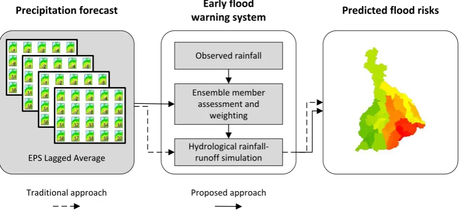
The overall methodology of the proposed approach is depicted inFigure 1. A lagged average

of the ensemble prediction members is usually used as an input to hydrological rainfall-runoff

simulations in order to predict flood risks. The objective of the proposed approach, however,

is to use observed rainfall data in order to identify the members with poor prediction quality.

Afterwards, the members are weighted according to their forecast skill with the aim of

improving the rainfall-runoff simulation. As a result, the outcome of the simulation would be

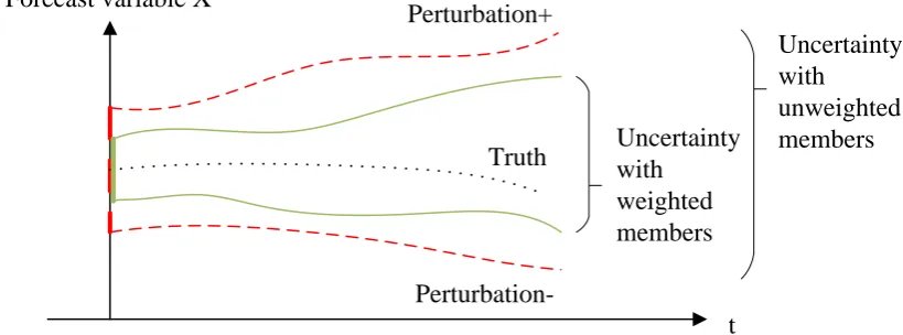
less uncertain or more accurate when using it in flood risk predictions (Figure 2).

EPS Lagged Average

Precipitation forecast Early flood

warning system

Ensemble member assessment and

weighting

Hydrological rainfall-runoff simulation

Predicted flood risks

Observed rainfall

Traditional approach Proposed approach

1 2 3 4 5 6 7 8 9 10 11 12 13 14 15 16 17 18 19 20 21 22 23 24 25 26 27 28 29 30 31 32 33 34 35 36 37 38 39 40 41 42 43 44 45 46 47 48 49 50 51 52 53 54 55 56 57 58 59 60 61

Truth Perturbation+

Perturbation-Uncertainty with

unweighted members Uncertainty

with weighted members Forecast variable X

t

Figure 2: Forecast uncertainty using unweighted and weighted ensemble members

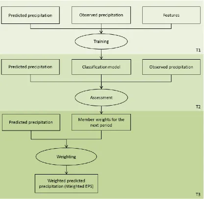
3.1. Ensemble member assessment and weighting

In order to assess ensemble members for future forecasts, real historical data is needed. The

assessment and weighting methodology is presented in Figure 3. Three time periods (i.e., T1,

T2 and T3) are considered. The precipitation predicted by the EPS for T1 and the observed

precipitation data for this period are used to train a machine learning classifier based on

features defined by hydrological experts. When new EPS data and observed precipitation data

arrives (T2), the generated classification model is applied in order to automatically assess the

prediction skills of the EPS members for this time period (and in the future). Thereby, the

members are weighted according to their skill. These weights are subsequently used for the

following/succeeding time period (T3), for which no observed data exists, because it is in the

future. The weighted EPS data for T3 is used as an input to a hydrological rainfall-runoff

1 2 3 4 5 6 7 8 9 10 11 12 13 14 15 16 17 18 19 20 21 22 23 24 25 26 27 28 29 30 31 32 33 34 35 36 37 38 39 40 41 42 43 44 45 46 47 48 49 50 51 52 53 54 55 56 57 58 59 60 61

Figure 3: Ensemble member assessment and weighting methodology

3.1.1. Ensemble member assessment

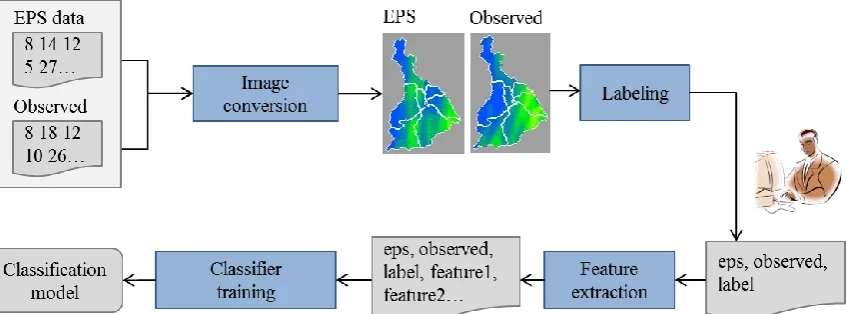
To automatically assess precipitation forecasts, a framework based on machine learning is

proposed (Figure 4). The framework consists of two tools – a training tool and an evaluation

tool, both implemented in Java. The training tool offers experts the opportunity to manually

label the prediction of an ensemble member at a certain point in time either as good or bad.

Usually, the forecast data for the different members and the observed rainfall data are in

matrix form, where each element represents a point in a numerical grid on which model

equations are solved. The training tool converts this data into images in order to enable direct

evaluation by experts. Different pixel colors indicate different precipitation values. The color

scheme is chosen according to the suggestion of the experts so that relevant differences or

1 2 3 4 5 6 7 8 9 10 11 12 13 14 15 16 17 18 19 20 21 22 23 24 25 26 27 28 29 30 31 32 33 34 35 36 37 38 39 40 41 42 43 44 45 46 47 48 49 50 51 52 53 54 55 56 57 58 59 60 61

rainfall well or not well and labels are generated. Afterwards, the evaluation tool extracts

features from the labeled data pairs.

Figure 4: Framework to create a machine learning classifier to identify low quality ensemble members

Since the landscape’s topography (e.g., elevation or river layout) plays a significant role

when an expert determines if the forecast data matches the observed rainfall data well, the

features used to classify forecasts should encode semantic knowledge about the

rainfall-runoff behavior of the entire area. Commonly, precipitation forecast areas are subdivided into

natural areas and sub-basins, taking into account hydrologically relevant characteristics, such

as altitude, climate and river layout. Based on the precipitation values (forecast and observed

data) and the defined areas, we propose the following features that are computed per area and

combined into a final feature vector. In the following equations, E is the EPS forecast, R

represents observed rainfall data, and i, j encode the pixel position in the image (i.e., the

position of the grid point in the numerical grid).

 Difference of the mean values per area (md)

(1)

 Difference of the standard deviations per area (sdd)

(2)

 Root-mean-square error per area (rmse)

(3)

1 2 3 4 5 6 7 8 9 10 11 12 13 14 15 16 17 18 19 20 21 22 23 24 25 26 27 28 29 30 31 32 33 34 35 36 37 38 39 40 41 42 43 44 45 46 47 48 49 50 51 52 53 54 55 56 57 58 59 60 61

(4)

The differences of the mean values per area (md, Eqn. 1) and the standard deviation per area

(ssd, Eqn. 2) are used to model the magnitude and spatial distribution, respectively, of

precipitation in a certain area. This information would be used by an expert to estimate how

much surface runoff will flow into a certain part of the river and eventually cause flooding.

Equation 3 (rmse) and Equation 4 (bcd) describe the general difference or dissimilarity

between areas as to model the overall similarity. These four features are used to train a

classifier and to generate a classification model.

3.1.2. Ensemble member weighting

Based on the classification model, other predictions can automatically be classified as good

or bad. The weights are calculated following an approach of Beven and Binley (1992).

Initially the GLUE (generalized likelihood uncertainty estimation) method was developed to

quantify uncertainty in hydrological modelling based on the assumption that different model

parametrizations result in equally good model performances. Then, the different

parametrizations are assigned to different weights in form of different likelihoods. In this

case, likelihood expresses a general measure of model performance or acceptance. In our

method we do not assume different model parametrizations, but different model inputs in

form of different EPS members.

Usually, EPS forecasts are released at certain time intervals with several lead ranges. In order

to investigate the differences between forecasts with short and long lead ranges, the skills of

the EPS members are weighted differently for the diverse lead ranges.

The evaluation tool counts the number of good predictions made by an EPS member based on

corresponding classification results for a certain time period. Depending on the number of

true positives (TP) and true negatives (TN), i.e., all correctly predicted forecasts per member,

the evaluation tool calculates a measure of the skill of each member M for range t, which

is equal to the ratio of the good predictions to all predictions (including the false positives FP

and false negatives FN) that belong to this member M,

1 2 3 4 5 6 7 8 9 10 11 12 13 14 15 16 17 18 19 20 21 22 23 24 25 26 27 28 29 30 31 32 33 34 35 36 37 38 39 40 41 42 43 44 45 46 47 48 49 50 51 52 53 54 55 56 57 58 59 60 61

Based on this skill, for each range t a likelihood measure Ft,M is assigned to every member M

as

(6)

According to Equation 6, a likelihood measure of zero is assigned to the worst member for

every range, while the best member will have a likelihood measure of 1. To use these

likelihoods as weights for the rainfall-runoff simulations, they have to be normalized, so that

the likelihoods in every range sum up to 1.0.

, , 20

, 1







t M t M

t M M

F L

F (7)

3.2. Hydrological rainfall-runoff simulation

For flood forecasting, the precipitation based on the numerical weather predictions has to be

transferred to runoff using a hydrological rainfall-runoff simulation model. This model,

however, has to be calibrated for a specific area that is considered.

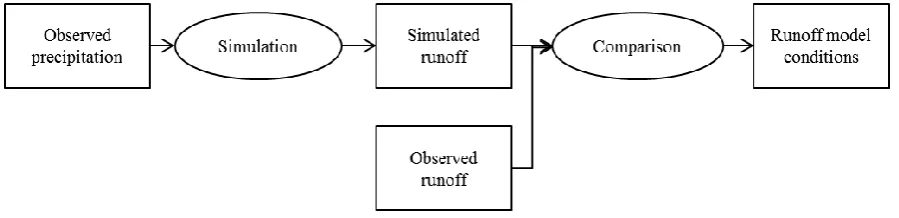
3.2.1. Calibration of the runoff model

The initial runoff model conditions, for example the soil moisture content at the time a

forecast is released, have to be known in order to guarantee accurate runoff simulations with

the EPS forecasts. To obtain these initial values, observed precipitation data is used as input,

as shown in Figure 5. A model is run with this observed data and the resulting simulated

runoff is compared to the actually observed runoff for this area and time period. Based on this

comparison, the optimal model conditions are derived and used afterwards as initial

conditions for succeeding simulations with the runoff model for the specific area.

Figure 5: Calibration of the runoff model

Different performance criteria are usually used to evaluate the model during calibration. To

1 2 3 4 5 6 7 8 9 10 11 12 13 14 15 16 17 18 19 20 21 22 23 24 25 26 27 28 29 30 31 32 33 34 35 36 37 38 39 40 41 42 43 44 45 46 47 48 49 50 51 52 53 54 55 56 57 58 59 60 61

used (Nash und Sutcliffe 1970). The NSE is dimensionless and scaled between minus infinity

and 1.0. It is obtained by dividing the mean square error of the observed and simulated data

by the variance of the observed data, subtracted from 1.0 (Equation 8).













obs t sim t t

n

obs t obs t

Q Q

NSE

Q μ

, (8)

where n is the total number of time steps, Qobs is the observed runoff at time step t, Qsim is the

simulated runoff at time step t, and μobs is the mean of the observed values. Furthermore, we

used the three Kling-Gupta coefficients α, β, and R² (Gupta et al. 2009), where α is the ratio

of the standard deviations of the simulated and observed runoff σsim and σobs (Equation 9), β is

the ratio of the mean simulated and mean observed runoff μsim and μobs (Equation 10), and R²

is the coefficient of determination of the simulated and observed runoff values (Equation 11),

 sim

obs

σ α

σ , (9)

 sim

obs

μ β

μ . (10)





















obs t obs sim t sim t

n n

obs t obs sim t sim

t t

Q μ Q μ

R

Q μ Q μ

(11)

R² is used to evaluate the timing and the shape of the flood wave, volumetric errors can be

assessed by β, while α provides conclusions related to the dynamics of the event. All

performance criteria have their optimum value at 1.0.

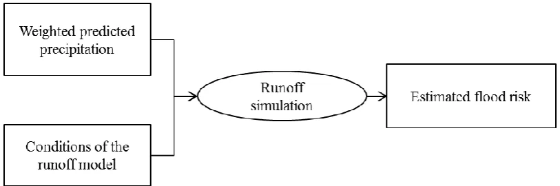
3.2.2. Flood risk estimation

The ensemble forecasts generated by the EPS are integrated into a flood early warning system

for an estimation of the current flood risk, as shown in Figure 6. To this end, a simulation of

the runoff is executed with the weighted predicted precipitation forecasts as input. Thereby,

the model conditions derived after calibration based on past periods are utilized as initial

conditions for the simulation run. Finally, the median of the simulated runoff is used to

1 2 3 4 5 6 7 8 9 10 11 12 13 14 15 16 17 18 19 20 21 22 23 24 25 26 27 28 29 30 31 32 33 34 35 36 37 38 39 40 41 42 43 44 45 46 47 48 49 50 51 52 53 54 55 56 57 58 59 60 61

Figure 6: Flood risk estimation methodology

4. CASE STUDY

In order to validate the approach a case study has been conducted. After introducing the

specific EPS and the specific river basin used in this study, the ensemble member assessment

and weighting procedure is exemplified followed by hydrological rainfall-runoff simulation.

4.1. COSMO-DE-Ensemble prediction system

The ensemble prediction system used in this study is named COSMO-DE-EPS (Consortium

for Small Scale Modelling–Deutschland–Ensemble Prediction System) and it is provided by

the German Weather Service (Baldauf et al. 2011). Every ensemble member includes

variations of lateral boundary conditions, initial conditions and model physics. The variations

of the lateral boundary conditions and the initial conditions are based on forecasts of four

different global models, which leads to a boundary condition ensemble prediction system

(BCEPS). The perturbation of the model physics is based on different configurations of the

COSMO-DE-EPS model, nested in the BCEPS. In every configuration, only one parameter is

modified. At the end, 20 ensemble members are produced. They are released eight times a

day, providing 27 hours of forecast lead time (Theis et al. 2012).

To verify the quality of the COSMO-DE-EPS regarding operational use in flood forecasting,

ensembles of the flood event of June 2013 in the Mulde river basin are evaluated. For this

purpose, the COSMO-DE-EPS results are compared with RADOLAN (Radar Online

Adjustment Procedure) data of the German Weather Service. The RADOLAN data combines

a real-time precipitation analysis based on weather radar products with an online adjustment

with rain gauges (Bartels 2004).

1 2 3 4 5 6 7 8 9 10 11 12 13 14 15 16 17 18 19 20 21 22 23 24 25 26 27 28 29 30 31 32 33 34 35 36 37 38 39 40 41 42 43 44 45 46 47 48 49 50 51 52 53 54 55 56 57 58 59 60 61

In this approach the study area is the Mulde River basin up to the gauge Bad Düben in

Saxony, Germany. The catchment has an area of approx. 6170 km² and can be separated into

three sub-basins. Shown in Figure 7 (right), from west to east these are the basins of the

tributaries Zwickauer Mulde, the rivers Zschopau and Flöha and the Freiberger Mulde. These

rivers converge and form the Vereinigte Mulde. The topography of the catchment can mainly

be subdivided into three natural spaces, which are different in their hydrological

characteristics. From south to north these are the landscapes of the Ore Mountain, the Saxon

Uplands and the Saxon Lowlands.

Figure 7: Mulde basin divided into sub-basins and natural spaces (left) and catchment areas (right)

To maintain the hydrologic interactions between sub-basins (e.g. fallen precipitation in

upstream areas have an impact on the downstream areas) and the climatological aspects (e.g.

the influence of the altitudes on the process of precipitation forming) of the different natural

areas, the Mulde basin is divided into seven parts based on the intersection of the sub-basins

and the borders of the natural areas. In order to consider this division, the features proposed

1 2 3 4 5 6 7 8 9 10 11 12 13 14 15 16 17 18 19 20 21 22 23 24 25 26 27 28 29 30 31 32 33 34 35 36 37 38 39 40 41 42 43 44 45 46 47 48 49 50 51 52 53 54 55 56 57 58 59 60 61

4.3. Ensemble member assessment and weighting

4.3.1. Ensemble member assessment

In this study, the Waikato Environment for Knowledge Analysis (WEKA) is utilized as a

machine-learning workbench in order to generate a classification model (Witten et al. 2011).

WEKA offers a collection of state-of-the-art machine learning algorithms. In addition, a Java

library is provided for embedded usage of the machine learning algorithms. WEKA provides

an opportunity to test different machine learning classifiers on a dataset. Also, methods that

evaluate the classifiers statistically and visualize the input data and the result of the learning

are supported.

There exist several ways to evaluate the performance of machine learning classifiers. One

commonly applied approach is to split labeled data into a training dataset and a test dataset.

Two thirds of the data are used for training and the remaining one third is used for testing.

However, the sample used for training may not be representative.

To mitigate any bias caused by the particular sample chosen for comparing the performance

of the different classifiers, 10-fold cross-validation is applied. The cross-validation ensures

that the results do not depend on chance effects. In case of limited training and test datasets,

the cross-validation guarantees that the results obtained for the specified test set would be the

same as results obtained by independent test sets. The main idea behind 10-fold

cross-validation is to split the data into ten approximately equal partitions (10 folds). Then, one

partition is used as test dataset and the other nine of the ten partitions are used as training

dataset. An error rate is calculated for the particular combination. This process is repeated ten

times with different partitions chosen as test dataset. At the end, the error estimates are

averaged in order to calculate the overall error estimate.

The percentage of correctly classified instances, precision and recall are chosen to evaluate

the capability of the classifiers to accurately classify test instances. Precision is calculated

according to Equation 12, while recall is calculated according to Equation 13.

(12)

1 2 3 4 5 6 7 8 9 10 11 12 13 14 15 16 17 18 19 20 21 22 23 24 25 26 27 28 29 30 31 32 33 34 35 36 37 38 39 40 41 42 43 44 45 46 47 48 49 50 51 52 53 54 55 56 57 58 59 60 61

In our study, 14,400 pairs of COSMO-DE-EPS and RADOLAN datasets are first converted

into text, and subsequently into images, since they are available only in GRIB2 code (General

Regulary-distributed Information in Binary form, Edition 2) as described by the World

Meteorological Organization (WMO 2003). In order to test and validate or classification

model, all of these image pairs are manually labeled by an expert in order to define the

ground truth. In a routine application, however, the expert would only label a portion of the

pairs required for training, while the rest of the forecasts would be classified automatically by

the assessment framework. In this case study the expert compares the intensities of the

precipitation, while taking into account the different areas of the Mulde basin. As a result, the

evaluation is tedious and it is not possible for an expert to continuously evaluate forecasts for

more than two hours a day.

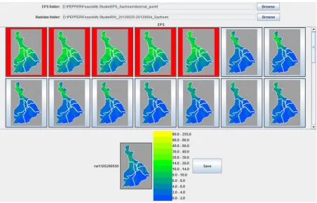
According to the expert’s opinion, 9,778 of the COSMO-DE-EPS results indicate good

forecasts. The remaining 4,622 COSMO-DE-EPS results are determined to be significantly

different from the RADOLANs in terms of assessing the precipitation. A screenshot of the

labeling process performed using the training tool is presented in Figure 8.

Figure 8: Screenshot of the training tool: Selection of EPS images (top, highlighted) not

1 2 3 4 5 6 7 8 9 10 11 12 13 14 15 16 17 18 19 20 21 22 23 24 25 26 27 28 29 30 31 32 33 34 35 36 37 38 39 40 41 42 43 44 45 46 47 48 49 50 51 52 53 54 55 56 57 58 59 60 61

WEKA implements a variety of machine learning methods and algorithms that differ both at

a conceptual or implementation level. Among this diversity, we choose three machine

learning methods, namely Support Vector Machines (SVM), Multilayer Perceptron, and

Rotation Forest.

Support vector machines are suitable for two-class datasets whose classes are linearly

separable (Witten et al. 2011). They combine linear modeling with instance-based learning.

Critical boundary instances, referred to as support vectors, are selected from each of the two

classes by a support vector machine. Based on these instances, a linear discriminant function

is built. This function defines a hyperplane which separates the support vectors as widely as

possible. The hyperplane is called the maximum-margin hyperplane, because it gives the

greatest separation between the classes. The SVM implemented in WEKA supports various

formulations. In our case study, we used C-Support Vector Classification (Chang & Lin

2011). The support vector machine classified 89% of the images correctly, leading to a

precision of 0.882 and a recall of 0.968 (Table 1).

There exist classifiers that can be applied also in cases when the data is not linearly separable

(Witten et al. 2011). For example, multilayer perceptrons are capable of coping with linearly

non-separable problems. Multilayer perceptrons are feed-forward artificial neural networks

(ANN). A perceptron is an online-learning algorithm, which means that it does not consider

the entire dataset at the same time, but it processes the training instances one by one.

Thereby, it generates a weight vector for the attributes of the training instances. The

perceptron makes a prediction for the affiliation of a given instance to a certain class based on

the weights learned so far and checks if this instance was classified correctly. If the instance

was misclassified, the weights vector is updated. A multilayer perceptron is a neural network

which consists of neurons aligned in layers (an input layer, one or several hidden layers, and

an output layer). Given a fixed network structure, the weights can be determined using

back-propagation.

The Multilayer Perceptron classifier achieved a precision of 0.885 using one hidden layer

with 15 nodes. A validation threshold of 20 is used to terminate validation testing, which

means that the validation set error can deteriorate 20 consecutive times before training is

stopped. The number of epochs (i.e., passes taken through the data) is 500 and the learning

rate which determines the step size is 0.3.

Rotation Forest is a classifier ensemble method based on feature extraction (Rodriguez &

1 2 3 4 5 6 7 8 9 10 11 12 13 14 15 16 17 18 19 20 21 22 23 24 25 26 27 28 29 30 31 32 33 34 35 36 37 38 39 40 41 42 43 44 45 46 47 48 49 50 51 52 53 54 55 56 57 58 59 60 61

over the individual classifier models. Lately, multiple classifier systems consisting of

classifiers trained on different data subsets or feature subsets have been designed. Commonly

called classifier ensembles, these classifiers are constructed by taking bootstrap samples of

objects and training a classifier on each sample. Then, the classifiers are combined using

majority voting.

Specifically, in Rotation Forest the feature set is randomly split into subsets and principal

component analysis is applied to each subset. After that, a new extracted feature set is

reassembled and the training data is transformed into the new features. The latter are used to

train decision tree classifiers, whereby each split of the feature set leads to a different

classifier. Each classifier calculates for a new instance the probability that the instance

belongs to a certain class. Then, the outputs of the classifiers are combined and the

probability assigned to an instance by the Rotation Forest is calculated using an average

combination method. In our case, the C4.5 decision trees is used (Quinlan 1993) and the

probabilities for the instances are calculated by 10 base classifiers.

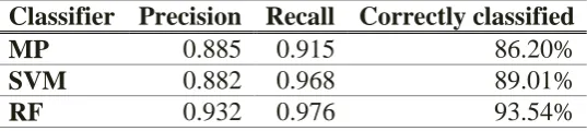
The results of the 10-fold cross-validation are presented in Table 1. Compared to the

Multilayer Perceptron (MP) and the Support Vector Machine (SVM), the Rotation Forest

(RF) classifier achieve the best results. It classifies correctly 94% of the EPS-RADOLAN

pairs. The Rotation Forest reaches a precision of 0.932 and a recall of 0.976. All three

measures validate that most of the forecasts are classified correctly.

Table 1: Classification performance for different classifiers

Classifier Precision Recall Correctly classified

MP 0.885 0.915 86.20%

SVM 0.882 0.968 89.01%

RF 0.932 0.976 93.54%

4.3.2. Ensemble member weighting

In order to prove that using the classifier can reduce the uncertainty of the flood forecast, the

ensemble members are assigned weights derived from the knowledge of the classifier tool.

In this approach, the EPS-RADOLAN pairs assessed by the classifier are sums over three

hours. So, for every released forecast, each member produces 9 three-hour-sums (range 1-3 h,

range 4-6 h... up to range 25-27 h) to be assessed by the tool. The capabilities of the 20

members are evaluated separately for all 9 time spans in order to investigate the differences

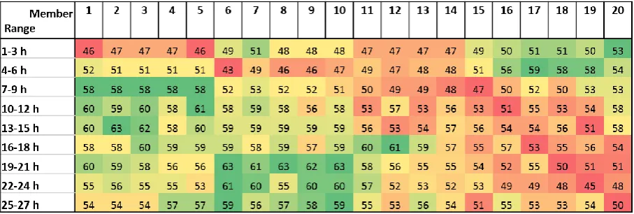
1 2 3 4 5 6 7 8 9 10 11 12 13 14 15 16 17 18 19 20 21 22 23 24 25 26 27 28 29 30 31 32 33 34 35 36 37 38 39 40 41 42 43 44 45 46 47 48 49 50 51 52 53 54 55 56 57 58 59 60 61

The results are shown in Figure 9, where the best forecasts per range are presented in green

and the worst ones in red. The available maximal value in Figure 9 is 80, as 80 forecasts are

evaluated per time span and member. The value 46 for member 1 for the range of 1-3 hours,

for example, means that 46 of the 80 forecasts are correctly predicted.

Figure 9: Evaluation of the skill of the 20 EPS members for different lead times

The corresponding likelihood weights L are shown in Figure 10. Since the classifier tool is

applied on three-hour-sums, the weights are always constant over a three-hour time span.

Figure 10: Weights derived from the evaluation tool for every member and every range

Now these likelihood weights can be used to reduce the predicted uncertainty range of the

flood forecast.

4.4. Hydrological rainfall-runoff simulation

In this study, we use the HBV-96 hydrological model (Lindström et al. 1997) in a software

implementation by Tyralla und Schumann (2013) for runoff simulation. The used model is

divided into 39 subareas up to the gauge Bad Düben 1. For the evaluation process the gauges

that best represent the structure of the natural spaces are selected. These gauges are shown in

Figure 7 (on the right).

1 2 3 4 5 6 7 8 9 10 11 12 13 14 15 16 17 18 19 20 21 22 23 24 25 26 27 28 29 30 31 32 33 34 35 36 37 38 39 40 41 42 43 44 45 46 47 48 49 50 51 52 53 54 55 56 57 58 59 60 61

An existing HBV-96 model of the River Mulde basin is recalibrated for the flood event in

June 2013 and for the application of the hourly values of the RADOLAN data.

Table 2 shows the model performance after the calibration process for the flood event in June

2013 with hourly RADOLAN data. All performance criteria values are in the upper range

near 1.0. Since there are no observed runoffs at the gauges Mahlitzsch and Großsermuth for

this event, no performance criteria for model evaluation can be calculated for these gauges.

Table 2: Model performance after the calibration for the flood event in June 2013 with hourly RADOLAN data

Gauge NSE β α R2

Zwickau-Pölbitz 0.98 0.95 0.91 0.99

Kriebstein UP 0.97 0.99 0.88 0.98

Hopfgarten 0.95 0.96 0.86 0.97

Borstendorf 0.96 0.96 0.90 0.97

Berthelsdorf 0.96 0.95 0.92 0.97

As shown in Figure 11, exemplarily for the gauges Zwickau-Pölbitz (river Zwickauer Mulde)

and Kriebstein UP (river Zschopau), the simulated hydrographs provide a good fit to the

observed hydrographs.

Figure 11: Observed and simulated hydrographs for the gauges Zwickau-Pölbitz (above) and Kriebstein UP (below)

1 2 3 4 5 6 7 8 9 10 11 12 13 14 15 16 17 18 19 20 21 22 23 24 25 26 27 28 29 30 31 32 33 34 35 36 37 38 39 40 41 42 43 44 45 46 47 48 49 50 51 52 53 54 55 56 57 58 59 60 61

An example of a simulation run with all 20 EPS members of one forecast at gauge Kriebstein

UP is shown in Figure 12. The release time t0 of this forecast is 2013-06-01T03:00. The grey

shaded area indicates the uncertainty range of the EPS members of this forecast run. The

dotted lines show the forecasts of every single member. The corresponding performance

criteria (defined in Eqn. 8-11) between the EPS forecast and the RADOLAN data as a

reference product are listed in Table 3. While the best members fit the RADOLAN reference

and the observed hydrograph well, the worst members overestimate the upcoming event

concerning flood peak and volume. At the time of the forecast release t0 all upcoming future

events are unknown. Thus, the uncertainty range leaves plenty of room for interpretation by

experts.

Figure 12: Simulation run of all 20 EPS member at gauge Kriebstein UP, release time 2013-06-01 03:00

Table 3: Performance criteria of the EPS forecast simulation at gauge Kriebstein UP, release time 2013-06-01 03:00

Best Worst Mean

NSE [-] 0.947 -22.719 -4.376

β [-] 1.005 1.824 1.276

α [-] 1.015 5.071 2.209

R² [-] 0.997 0.677 0.909

Throughout the whole duration of this event, the uncertainty range of all EPS forecasts for the

gauge Kriebstein UP is shown in Figure 13. The envelope of the uncertainty range is

calculated by using the minimum and maximum forecasted runoff value for each time step,

1 2 3 4 5 6 7 8 9 10 11 12 13 14 15 16 17 18 19 20 21 22 23 24 25 26 27 28 29 30 31 32 33 34 35 36 37 38 39 40 41 42 43 44 45 46 47 48 49 50 51 52 53 54 55 56 57 58 59 60 61

the runoff simulations using the predictions made by the whole example indicates that the

EPS forecasts tend to more likely overestimate the precipitation than to underestimate it.

Figure 13: Overall uncertainty range at gauge Kriebstein UP

For each time step in every simulated forecast run, the predicted runoff values are sorted in

ascending order, while the corresponding likelihood weights are accumulated. Figure 14

shows an example for the forecast of the release time 2013-06-01T03:00 at gauge Kriebstein

UP, with predicted runoff values at 2013-06-02T02:00 and the associated weights of range 21

h. Due to the prior knowledge that the ensemble forecast overestimates and underestimates

the observed runoff on a large scale, upper and lower tolerance limits can be assigned to the

band of uncertainty in form of quantile thresholds. The limits of this inter-quantile range can

be freely chosen, based on the experience of the experts. In this approach, the 25% and 75%

1 2 3 4 5 6 7 8 9 10 11 12 13 14 15 16 17 18 19 20 21 22 23 24 25 26 27 28 29 30 31 32 33 34 35 36 37 38 39 40 41 42 43 44 45 46 47 48 49 50 51 52 53 54 55 56 57 58 59 60 61

Figure 14: Cumulative likelihoods and predicted runoff values at 2013-06-02T02:00 (forecast release at 2013-06-01T00:00, forecast range 21 h) for weighted and unweighted

members at gauge Kriebstein UP

As Figure 14 shows, assigning weights to the predictions of the corresponding members

reduces the outer bound of the uncertainty range. Treating all members equally, the 75%

quantile value is approximately 650 m³/s, while the corresponding weighted quantile value is

approximately 440 m³/s when weighted members are used. The weighted lower boundary is

nearly unchanged. Given that the observed runoff value at this time step is 349 m³/s and the

overestimation is greater than the underestimation, the reduction of the uncertainty range in

this way is reasonable.

To compare the whole forecast period of the weighted and restricted uncertainty range for the

release time 2013-06-01T03:00 at gauge Kriebstein UP with the uncertainty range of the

original forecast, the corresponding hydrograph is plotted in Figure 15. It shows the same

forecast like the one presented in Figure 12, but this time the reduced uncertainty range

derived from the classifier tool is plotted in dark grey. The calculated performance criteria are

1 2 3 4 5 6 7 8 9 10 11 12 13 14 15 16 17 18 19 20 21 22 23 24 25 26 27 28 29 30 31 32 33 34 35 36 37 38 39 40 41 42 43 44 45 46 47 48 49 50 51 52 53 54 55 56 57 58 59 60 61

Table4, where Q25 reflects the performance of the lower bound of the weighted uncertainty

range and Q75 of the upper bound, respectively. The weighted median is shown in red and

matches the RADOLAN reference and the observed hydrograph well.

Figure 15: Enhancement of the forecast skill by using weighted quantiles (Q25 and Q75) derived from the classifier tool (dark grey area) at gauge Kriebstein UP, release time

1 2 3 4 5 6 7 8 9 10 11 12 13 14 15 16 17 18 19 20 21 22 23 24 25 26 27 28 29 30 31 32 33 34 35 36 37 38 39 40 41 42 43 44 45 46 47 48 49 50 51 52 53 54 55 56 57 58 59 60 61

Table 4: Performance criteria of the weighted EPS forecast simulation at gauge Kriebstein UP, release time 2013-06-01T03:00

Q25 Q75 Median

NSE [-] 0.852 -2.892 0.891

β [-] 0.927 1.362 1.054

α [-] 0.781 2.575 1.119

R² [-] 0.946 0.986 0.943

To evaluate the classification tool for the whole event, the weighting procedure is applied for

every EPS runoff forecast using the 25% and 75% quantile as boundaries of the uncertainty

range. To have an appropriate comparison with Figure 13, for the restricted uncertainty range

every forecast is also superpositioned and the outermost Q25/Q75-value for every simulated

time step was chosen as the boundary for the dark grey area in Figure 16. Due to the

proposed method, the peak for the 2 June 2013 does not occur and several other peaks are

damped while the shape of the uncertainty band remains similar. This means that the required

level of uncertainty is still taken into account, while the peak and successive overestimated

probability of flood occurrence are eliminated.

1 2 3 4 5 6 7 8 9 10 11 12 13 14 15 16 17 18 19 20 21 22 23 24 25 26 27 28 29 30 31 32 33 34 35 36 37 38 39 40 41 42 43 44 45 46 47 48 49 50 51 52 53 54 55 56 57 58 59 60 61

5. CONCLUSIONS AND FUTURE WORK

In recent years, ensemble prediction systems (EPS) have been applied to limit the uncertainty

of hydrometeorological forecasts. An ensemble forecast represents a collection of two or

more forecasts conducted using slightly different model components, model parameters or

varying initial and boundary conditions. These forecasts are referred to as ensemble

members. Yet, the equal inclusion of skillful and less skillful members often leads to a too

wide uncertainty range, resulting in the over- or underestimation of the risk of floods or other

hazardous events.

To improve the performance of the forecasts, the skills of the ensemble members were

evaluated in this study. A framework based on machine learning was developed in order to

automate and accelerate the evaluation process. Based on labeled pairs of forecasted and

actual precipitation conditions, the framework is capable of evaluating the skill of different

ensemble members. A weighting procedure of the members with good performance was

carried out. The advantage of the proposed method is the automated, time-saving assessment

of the ensemble members, as soon as new observed precipitation is available. Consequently,

the weighting is an adaptive method. Would one member, for instance, always have a poor

prediction skill at specific forecast intervals, the weighting would gradually be reduced and

the influence in the forecasted uncertainty range would become smaller.

The contribution of the presented methodology is two-fold. On one hand, experts are assisted

while evaluating EPS forecasts by the use of an automated machine learning framework. On

the other hand, the results of the validation tests show that by weighting the ensemble

members appropriately, the uncertainty range in flood risk predictions is reduced, but still

sufficiently shaped in order to account for the model physics, initial and boundary conditions.

Therefore, the overall performance of the ensemble system is improved. The approach was

successfully validated against precipitation data of the Mulde river basin area in Germany for

the flood event in June 2013 using an ensemble system with 20 members.

The practical benefit for the people at the flood forecasting centers would be that each time

when a new ensemble forecast is released, all ensemble members are automatically assessed

and weighted, and the weighted ensemble can be used for assessing the flood risk. The

influence on the predicted uncertainty range of members which led to an underestimation or

exaggeration of an event in the past would decrease, thus the prediction of flood duration and

1 2 3 4 5 6 7 8 9 10 11 12 13 14 15 16 17 18 19 20 21 22 23 24 25 26 27 28 29 30 31 32 33 34 35 36 37 38 39 40 41 42 43 44 45 46 47 48 49 50 51 52 53 54 55 56 57 58 59 60 61

Yet, the approach presented in this paper still has some limitations. For example, it was

assumed that the weights of the members are independent of the meteorological conditions.

However, the behavior of the members may vary under different weather conditions.

To compensate this, future research may include a distinction between different

meteorological conditions. If it is foreseeable for the expert that the upcoming storm is a

convective precipitation event or an advective event, different model weights could be used.

Also, a higher weighting or selection of more recently released and correctly predicted

forecasts in form of a sub-ensemble is possible. To this end, it is necessary to investigate the

impact of the chosen time periods on the forecast performance. In addition, the methodology

1 2 3 4 5 6 7 8 9 10 11 12 13 14 15 16 17 18 19 20 21 22 23 24 25 26 27 28 29 30 31 32 33 34 35 36 37 38 39 40 41 42 43 44 45 46 47 48 49 50 51 52 53 54 55 56 57 58 59 60 61

REFERENCES

American Meteorological Society (AMS) (2000). Glossary of Meteorology, Second Edition Baldauf, M., Seifert, A., Förstner, J., Majewski, D., Raschendorfer, M. & Reinhardt, T.

(2011) Operational convective-scale numerical weather prediction with the COSMO model: Description and sensitivities, Monthly Weather Review 139 (12), pp. 3887–3905 Bartels H. (2004) Projekt RADOLAN, Routineverfahren zur Online-Aneichung der Radarniederschlagsdaten mit Hilfe von automatischen Bodenniederschlagsstationen (Ombrometer), final report. Offenbach: Deutscher Wetterdienst

Beven, K., Binley, A. (1992) The future of distributed models. Model calibration and uncertainty prediction. In: Hydrol. Process. 6 (3), pp. 279–298.

Brochero, D., Anctil, F. & Gagne, C. (2011) Simplifying a hydrological ensemble prediction system with a backward greedy selection of members – Part 1: Optimization criteria.

Hydrology and Earth System Sciences 15, pp. 3307-3325

Casanova, S. & Ahrens, B. (2009) On the Weighting of Multimodel Ensembles in Seasonal and Short-Range Weather Forecasting. In: Mon. Wea. Rev. 137 (11), pp. 3811–3822. Chang, C.-C. & Lin, C.-J. (2011) LIBSVM: A library for support vector machines. ACM

Transactions on Intelligent Systems and Technology 2 (3)

Cloke, H.L. & Pappenberger, F. (2009) Ensemble flood forecasting. A review, Journal of Hydrology 375, pp. 613–626.

Dietrich, J., Schumann, A. H., Redetzky, M., Walther, J., Denhard, M., Wang, Y., Pfützner, B. & Büttner, U. (2009) Assessing uncertainties in flood forecasts for decision making: prototype of an operational flood management system integrating ensemble predictions.

Natural Hazards and Earth System Sciences 9, pp. 1529-1540

Eckel, F. A. & Walters, M. K. (1998) Calibrated Probabilistic Quantitative Precipitation Forecasts Based on the MRF Ensemble. Weather and Forecasting 13, pp. 1132-1147 Evans, J. P., Ji, F., Abramowitz, G. & Ekström, M. (2013) Optimally choosing small

ensemble members to produce robust climate simulations. Environmental Research Letters 8

Gagne II, D. J., McGovern, A. & Xue, M. (2012) Machine Learning Enhancement of Storm Scale Ensemble Precipitation Forecasts. Conference on Intelligent Data Understanding (CIDU), pp. 39-46

Garaud, D. & Mallet, V. (2011) Automatic calibration of an ensemble for uncertainty estimation and probabilistic forecast: Application to air quality. Journal of Geophysical Research 116

Gneiting, T., Raftery, A. E., Westveld, A. H. & Goldman, T. (2005) Calibrated Probabilistic Forecasting Using Ensemble Model Output Statistics and Minimum CRPS Estimation. In: Mon. Wea. Rev. 133 (5), S. 1098–1118.

Gupta, H. V., Kling, H., Yilmaz, K. K. and Martinez, G. F. (2009) Decomposition of the mean squared error and NSE performance criteria: Implications for improving hydrological modelling. Journal of Hydrology, 377 (1-2), 80–91. doi:10.1016/j.jhydrol.2009.08.003.

Hamill, T. M. & Juras, J. (2006) Measuring forecast skill: is it real skill or is it the varying climatology? Quarterly Journal of the Royal Meteorological Society 132(621C), pp. 2905-2923

Hamill, T. M. & Swinbank, R. (2014) Stochastic forcing, ensemble prediction systems, and TIGGE. World Weather Open Science Conference 2014, Montreal, Canada

Keil, C., Craig, G. C. (2009) A Displacement and Amplitude Score Employing an Optical Flow Technique. In: Wea. Forecasting 24 (5), S. 1297–1308.

1 2 3 4 5 6 7 8 9 10 11 12 13 14 15 16 17 18 19 20 21 22 23 24 25 26 27 28 29 30 31 32 33 34 35 36 37 38 39 40 41 42 43 44 45 46 47 48 49 50 51 52 53 54 55 56 57 58 59 60 61

Krishnamurti, T. N. (1999): Improved Weather and Seasonal Climate Forecasts from Multimodel Superensemble. In: Science 285 (5433), S. 1548–1550.

Lindström, G., Johansson, B., Persson, M., Gardelin, M. and Bergström, S. (1997) Develop-ment and test of the distributed HBV-96 hydrological model. Journal of Hydrology, 201 (1-4), 272–288. doi:10.1016/S0022-1694(97)00041-3.

Mallet, V., Stoltz, G. & Mauricette, B. (2009) Ozone ensemble forecast with machine learning algorithms. Journal of Geophysical Research 114

Nash, J. E. and Sutcliffe, J. V., 1970. River flow forecasting through conceptual models part I — A discussion of principles. Journal of Hydrology, 10 (3), 282–290. doi:10.1016/0022-1694(70)90255-6.

National Weather Service, Weather prediction Center (WPC) (2006) Ensemble Prediction Systems: A basic training manual targeted for operational meteorologists. Online, available at: http://www.wpc.ncep.noaa.gov/ensembletraining/, accessed on 14.04.2015 Quinlan, J. R. (1993) C4.5: programs for machine learning. Morgan Kaufmann Publishers

Inc. San Francisco, CA, USA

Raftery, A. E.; Gneiting, T., Balabdaoui, F. & Polakowski, M. (2005) Using Bayesian Model Averaging to Calibrate Forecast Ensembles. In: Mon. Wea. Rev. 133 (5), S. 1155– 1174.

Rodriguez, J. J. & Kuncheva, L. I. (2006) Rotation Forest: A New Classifier Ensemble Method. IEEE Transactions on Pattern Analysis and Machine Intelligence 28(10), pp. 1619-1630

Schumann, A.H., Wang, Y. & Dietrich, J. (2011) Framing uncertainties in flood forecasting with ensembles. Hydrology for Flood Risk Assessments and Management, Springer-Publishing Company

Schüttemeyer, D. & Simmer, C. (2011) Uncertainties in Weather Forecast – Reasons and Handling. In: Andreas H. Schumann (Hg.): Flood Risk Assessment and Management. Dordrecht: Springer Netherlands, pp. 11–33.

Sloughter, J. Mc Lean; Raftery, Adrian E.; Gneiting, Tilmann; Fraley, Chris (2007) Probabilistic Quantitative Precipitation Forecasting Using Bayesian Model Averaging. In: Mon. Wea. Rev. 135 (9), S. 3209–3220.

Theis, S., Gebhardt, C. & Bouallègue, Z. B. (2012) Beschreibung des COSMO-DE-EPS und seiner Ausgabe in die Datenbanken des DWD, Version 1.0. Offenbach: Deutscher Wetterdienst

Tyralla, C., Schumann, A. (2013) HydPy - ein interaktiv nutzbares Framework zur Erstellung und Anwendung hydrologischer Modelle. Hg. v. Bundesanstalt für Gewässerkunde. Bundesanstalt für Gewässerkunde (1795).

Wealands, S.R., Grayson, R.B. & Walker, J.P. (2003) Hydrologic model assessment from automated spatial pattern comparison techniques, Proceedings of the International Congress on Modelling and Simulation, Australia, 2003, pp. 426-42

Weusthoff, Tanja; Leuenberger, Daniel; Keil, Christian; Craig, George C. (2011) Best Member Selection for convective-scale ensembles. In: Meteorol. Z. 20 (2), S. 153–164. Williams, J. K., Ahijevych, D. A., Kessinger, C. J., Saxen, T. r., Steiner, M. & Dettling, S.

(2008) A machine learning approach to finding weather regimes and skillful predictor combinations for short-term storm forecasting. 13th Conference on Aviation, Range and Aerospace Meteorology, New Orleans, LA, American Meteorological Society Witten, I. H., Frank, E. & Hall, M. A. (2011) Data mining: practical machine learning tools

and techniques, Elsevier