Maintenance processes modelling and optimisation

MAINTENANCE PROCESSES MODELLING AND

OPTIMISATION

Yang, Zhang*_{, John Andrews}*,1_{, Sean, Reed}* _{& Magnus, Karlberg}** * _{Resilience Engineering Research Group, University of Nottingham, UK}

** _{Faste Laboratory, Lulea University of Technology, Sweden} 1_{CorrespondingE-Mail: [email protected]}

Abstract

A Maintenance Procedure (MP) is conducted in order to prevent the failure of a system or to restore the functionality of a failed system. An MP consists of a series of tasks, each of which has a distribution of times to complete and a probability of being performed incorrectly. The inclusion of tests in an MP can be used to identify any maintenance errors which have occurred. When an error is identified it can be addressed through a corresponding correction sequence which will have associated costs and add into the duration of the MP completion. A modified FMEA approach has been used to identify the possible tests. By incorporating any selection of tests into the MP it is then subjected to a discrete-event simulation to predict the expected completion time distribution. The choice of tests to perform and when to do them is then made to successfully complete the MP’s objective in the shortest possible time using a genetic algorithm. The methodology is demonstrated by applying it to the repair process for a car braking system. The developed method is suitable for application in abroad range of industries.

Key Words: Maintenance, Optimisation, Failure Mode and Effect Analysis, Discrete-event simulation, Genetic algorithm, System availability

1

INTRODUCTION

In order to repair hardware failures and restore functionality of hardware, a maintenance procedure (MP) is performed by a sequence of tasks [1]. It may be possible to perform a task incorrectly or for a task to take too long to complete. Since there is frequently a time limit on the window of opportunity to conduct the repair, both of the undesirable outcomes can be considered as failures of the MP. Therefore, the objective of this research is to develop a means by which any task failure occurring during performance of an MP can be identified and subsequently rectified to restore the hardware functionality in as short a time as possible.

are needed to find a good solution within a reasonable time and computational effort [3]. An optimal combination of tests is required, which can then be integrated within the process design to achieve its objective in the shortest time.

The modelling framework developed is appropriate for application in any industry since minimising the maintenance activity time will increase the availability of the system. Recently there has been a trend towards functional products [4], or power by the hour type contractual arrangements where a capability is sold rather than a product. The responsibility for the maintenance within such contracts rests with the supplier rather than the purchaser and a major factor influencing the financial success will be the effectiveness and efficiency with which the repairs can be carried out. The modelling approach developed has the potential to make a significant impact in such industries.

In order to illustrate the methodology established to develop a test selection strategy, a car braking system repair process is considered. The layout of the paper is as follows: Section 2 gives a detailed description of the braking system repair process example. In Section 3, a modified FMEA technique is described which identifies faults or failures introduced during the braking system repair process. By applying this, a full set of potential testing options is established. The simulation method used to predict the expected MP execution time and an optimisation strategy, in which the analysis model is embedded with the testing options selected is then described in the next section. The analysis results are then shown in Section 5 and conclusions are drawn in Section 6.

2

CAR BRAKING SYSTEM MAINTENANCE PROCESS

A car braking system is used to slow or stop a moving vehicle, which is usually accomplished by means of friction [5]. The front brakes of a car are more significant than the rear brakes when stopping the car, since the braking process transfers the car’s weight onto the front wheels and increases the available grip. In the event that the braking system needs maintenance due to worn-out brake-pads and rotor located on the front left wheel of a car. The objective of the motor mechanic is to replace the worn-out brake pads and rotor so that the braking system is restored to its functional state. At the end of the process, a driving test is performed to ensure the braking system is fully functioning. Theoretically, an MP can always achieve its objective to restore system functionality, assuming the presence of sufficient and reliable tests, and the variable is the time in which this will be achieved. Therefore, the expected time taken to accomplish the maintenance objective is the performance measure by which the efficiency of the MP will be evaluated.

2.1 The Hardware

Figure 1: The parts of a car braking system considered in the MP (Source: RepairPal.com [6]) 2.2 The Resources

There are three factors that contribute to the length of downtime of any failed hardware item: the preparation time for arranging the maintenance technicians; the actual MP performance time and the logistic time required to obtain any necessary maintenance resources [7]. The MP requires resources, either equipment or spares, at different stages of the repair process. In the example, there are two tools: a wrench and a jack, and four consumable spares: grease, new brake-pads, a new rotor and new wheel bolts. These resources are acquired before the MP starts (except the new wheel bolts, since they are not compulsory) and are ready to use when needed. One mechanic is required and is on-site when the repair starts.

2.3 The Required Maintenance Procedure Tasks

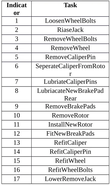
The braking system repair process has 20 standard process tasks, which, when required, are performed in sequence by the mechanic. The process tasks together with their indicator numbers are shown in Table I.

Table I: Basic tasks involved in the braking system repair process Indicat

or

Task

1 LoosenWheelBolts

2 RiaseJack

3 RemoveWheelBolts

4 RemoveWheel

5 RemoveCaliperPin

6 SeperateCaliperFromRoto r

7 LubriateCaliperPins 8 LubriacateNewBrakePad

Rear

9 RemoveBrakePads

10 RemoveRotor

11 InstallNewRotor

12 FitNewBreakPads

13 RefitCaliper

14 RefitCaliperPin

15 RefitWheel

16 RefitWheelBolts

18 TightenWheelbolts

19 CleanBrakePads

20 GetNewWheelbolts

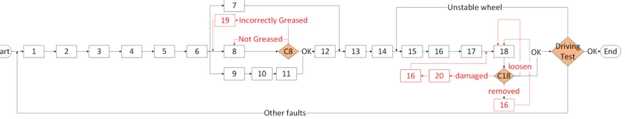
The process flow diagram that shows the sequence of tasks is given in Figure 2. Parallel sections indicate where there are several possibilities which can be performed depending upon the circumstamces. For example, after the performance of task 6, any of the three tasks: 7, 8 and 9, can be performed and the sequence in which they are conducted will not affect the progress of the overall MP. After the performance of task 8, a checking task C8 is perform to reveal if the new brake pads have been greased correctly and thus determine which task to perform next. If the brake pads are not greased, then task 8 is repeated; or if the brake pads are incorrectly greased (the front part rather than the rear parts are greased), then task 19 is performed. A similar checking task is conducted after the performance of task 18 to show the state of the wheel bolts. The actions which follow correspond to the different wheel bolts states. If both task 8 and task 11 is completed correctly, then the mechanic can progress to task 12.

Figure 2: Instruction of the braking system repair process with tasks represented by indicators in Table I

Before the end of the MP, a driving test (as described in Section 3.3) will be performed prior to discover any deviations from the correct states of the hardware for normal functionality of the system. If any deviation is detected, the appropriate rectification actions will be carried out to correct the problem, or alternatively the entire repair process needs to be repeated. The overall process ends when the driving test shows that the process has been completed correctly. The three checking tasks in the MP shown in Figure 2 are compulsory in order to ensure the progress of the MP and success of the MP objective.

3

USING THE MODIFIED FMEA TECHNIQUE TO IDENTIFY

FAULTS

new sequence of rectification tasks are conducted to achieve the objective of the process [3]. Here, a modified FMEA method is employed to model the MP case study.

3.1 Assumptions

The following assumptions are made in modelling the MP:

 There is one mechanic or one team performing the MP, the process tasks are then executed in a certain sequence one after another. Thus, the overall execution time is an accumulation of the execution time of all individual process tasks.

 The execution of a process task can change the state of a certain component in the hardware with a specific probability.

 The performance time of a task depends on the state of the affected hardware at the start of the task. The performance time can follow any distribution, in this braking system repair example, we assume it follow a normal distribution.

Consider for example, task 3 “remove wheel bolts”, the performance time depends on the state of the wheel bolts. The wheel bolts have four different possible states: ‘tight’, ‘loose’, ‘removed’ and ‘damaged’. If the state of the wheel bolts at the beginning of task 3 is ‘loose’, then, as shown in Table II, task 3 has a probability of 0.9 of changing the state of the wheel bolts from ‘loose’ to ‘removed’. The time needed to perform task 3 follows a truncated normal distribution [8] with mean 40 seconds(s) and standard deviation 8s. There is a 0.1 chance that the wheel bolts will remain in the ‘loose’ state. It can be seen that, conducting task 3 will not change the state of the wheel bolts from ‘loose’ to either ‘tight’ or ‘damaged’.

Table II: The states of wheel bolts changing from 'loosen' after the performance of task 3: ‘remove wheel bolts’ and their corresponding process time and probability

State change from ’loosen ’ to Tighten Loose n

Remove d

Damage d

Probability n/a 0.1 0.9 n/a

Time(s) n/a 0 N(40,8) n/a

 In order to initiate a process task, some prerequisite conditions, i.e., specific states of the hardware components involved are required. If these conditions are not true, this task will be neglected and no time is added to the overall execution time. Consider for example task 4 ‘remove the wheel’, the initiation of this task requires that the wheel bolts are ‘removed’ and the jack is ‘raised’. If either of these conditions is not satisfied, task 4 will be skipped, and the total process execution time and the state of the hardware component will remain unchanged.

 Incorrect ordering or neglect of tasks in the maintenance can potentially result in failure of maintenance objective.

3.2 The modified FMEA Method

The MP is analysed using a modified FMEA method where each maintenance task which forms a part of the MP is defined by:

 The name of the task.

 The resources and tools required (inputs of each task).

 The prerequisite conditions required in order to initiate the task.

 The outcomes of the task are mutually exclusive. Each outcome is defined by the state of the affected hardware component. The outcome specifies: the component state, its occurrence probability and the distribution of the time to perform the task.

 The local and global effect if the failure mode is ignored.

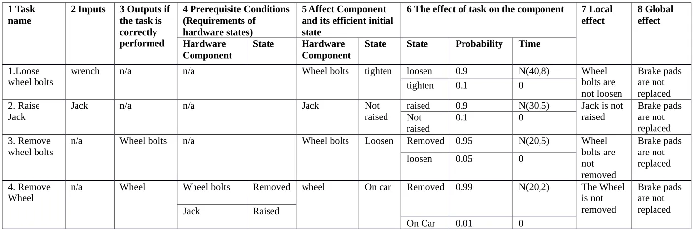
Each task in the process is analysed to identify all of the errors and failures which can occur and the consequences and associated symptoms are recorded in tabular form as described above. The information produced for some of the process tasks is illustrated in Table III. The first column gives the name of the task; the second column shows what resources or equipment the task requires and the third shows the outputs of this task; the fourth column lists the prerequisite conditions of the task, i.e. the specified hardware components and their required states. The task initiates only if the prerequisite conditions, if any, are satisfied. If the task is initiated, it changes the hardware component from one state to another with a specified probability. The component the task affects together with its initial state is shown in column 5. The state to which the component transfers after the performance of the task, along with its corresponding probability and time, is shown in column 6. The symptoms in the form of the local and global effects if the task fails are shown in columns 7 and 8 respectively.

As an example, consider task 4: ‘remove the wheel’. The task doesn’t require any extra resources. If task 4 is performed successfully, then there will be one output affecting the wheel. The initiation of this task requires two prerequisite conditions, i.e., the wheel bolts are ‘removed ’and jack is ‘raised’. The task will affect the state of the wheel if the wheel is ‘on car’ when the task starts. Otherwise if the wheel is already ‘removed’, the ‘remove the wheel’ task won’t change the state of the wheel and no time is added to the overall maintenance execution time. After the performance of the task, the state of the wheel may change from ‘on car’ to ‘removed’ with probability of 0.99, with the execution time sampled from a normal distribution, N(20, 2). There is a 0.01 chance that this task is forgotten, and then the wheel state and the overall time will not change. If the wheel is still ‘on car’, it means the task has failed and furthermore, it will lead to the failure of the whole MP to replace the brake pads and rotor.

3.3 Error Testing During the Braking System Repair Process

In order to illustrate the approach to select the optimal tests to identify failures and mistakes in the brake repair process, as many of the tests as possible are explored. There are many tests which can be performed but it will not be cost effective to choose them all since each test and its corresponding correction sequence costs time and will add to the total MP completion time. Therefore, for an effective overall process, a small subset of tasks needs to be identified which will provide the best benefit (measured as the least completion time to achieve the objective). Each different selection of tests leads to different process design with a different average completion time.

Each test will reveal the state of a hardware component. If the state revealed is not the desired one, then the corresponding corrective actions need to be carried to rectify the observed error. A test includes the behaviour to check the state of the hardware component and a sequence of corrective actions. It is possible for two tests to share an action of checking the state of the same component, but the rectification actions are different between the two tests due to varying the time point at which the tests are performed in the MP.

unstable, then the mechanic will repeat the MP from task 15: ‘refit the wheel’. For any other failures (such that the braking system still doesn’t work or noises occurring during the test), the mechanic starts over from the beginning and performs the tasks in sequence as shown in Figure 2.

Table III: The modified FMEA for task 1 to task 4 1 Task

name

2 Inputs 3 Outputs if the task is correctly performed

4 Prerequisite Conditions (Requirements of hardware states)

5 Affect Component and its efficient initial state

6 The effect of task on the component 7 Local effect

8 Global effect

Hardware

Component State HardwareComponent State State Probability Time

1.Loose

wheel bolts wrench n/a n/a Wheel bolts tighten loosen 0.9 N(40,8) Wheel bolts are not loosen

Brake pads are not replaced tighten 0.1 0

2. Raise

Jack Jack n/a n/a Jack Not raised raised 0.9 N(30,5) Jack is not raised Brake pads are not replaced Not

raised 0.1 0 3. Remove

wheel bolts n/a Wheel bolts n/a Wheel bolts Loosen Removed 0.95 N(20,5) Wheel bolts are not removed

Brake pads are not replaced loosen 0.05 0

4. Remove

Wheel n/a Wheel Wheel bolts Removed wheel On car Removed 0.99 N(20,2) The Wheelis not removed

Brake pads are not replaced Jack Raised

For the braking system repair process example, there are 20 possible tests that be included. Each test is defined by:

 the time needed to check the hardware state.

 the state of the hardware component which will indicate that, the process task has been correctly performed.

 the corrective actions corresponding to each possible failure state of the hardware component that the test can reveal.

For example, a test can be conducted after the performance of Task 4: ‘remove the wheel’ to detect its correct execution. The test, denoted as C4, will reveal the state of the wheel in order to judge whether task 4 is successfully completed. The information of this test is shown in Table IV.

Table IV: The Test that checks whether task 4:'remove the wheel' has been correctly completed Test

Indicator

Test name Time(s

)

The correct Possible

failure mode

Corrective actions Hardware

component

State

C4 Observe wheel

after task 4: ‘remove the wheel’

5 The wheel remove

d

On car Repeat task 4

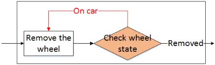
The action that checks the state of the wheel takes 5s. If the wheel is ‘removed’, then this means task 4 has been correctly completed. There is one possible failure state of the wheel, i.e., the wheel is still ‘on car’, meaning that task 4 is unsuccessful. If this failure state is detected, then the corresponding corrective action: repeat task 4, needs to be conducted until the correct wheel state is revealed. The flow chart of this process is shown in

.

Figure 3: The flowchart showing the process of test C4: observe the state of the wheel after task 4.

Table V: The test that checks whether task 15:'refit the wheel' has been correctly completed Test

Indicator

Test name Time(s

)

The correct Possible

failure mode

Corrective actions Hardware

component

State

C15 Observe wheel

after task 15:‘refit the wheel’

5 The wheel On

car

Removed Repeat task 15

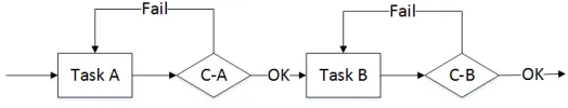
When the Tests are Introduced in the Maintenance Procedure: A test option, denoted as C-A, is introduced to verify whether task A has been correctly conducted. The check task can be performed immediately after the performance of task A or in a later stage. However, under the assumptions stated in Section 3.1, it is suggested the test C-A should be performed

immediately after task A, i.e., the tasks and follow-up tests should be arranged as illustrated in Figure 4 other than Figure 5.

Figure 4: Suggested tests position arrangement in the MP

Figure 5: A non-optimal tests position arrangement in the MP

This is due to the fact that the performance of a further process task B, after the failed task A, can possibly change the state of prerequisite conditions of task A and task C-A, such that C-A cannot be initiated in a later stage or lead to unnecessary repeats of process tasks.

4

PROPOSED OPTIMISATION MODEL

The integration of the standard maintenance process tasks along with a selection of optional tests forms the total process design. The expected completion time of execution of a braking system maintenance process design depends on the selection of tests. The tests incorporated can be optimised to find the process design that has the lowest execution time. The critical maintenance process design is that which incorporates tests such that it is optimal.

When the test options are limited, it is possible to evaluate all options exhaustively to find the optimal process design. In the more common, complex processes, where there are huge numbers of possible test process designs, a formal optimisation methodology such as the genetic algorithm is needed to find a good solution within a reasonable amount of time and computational effort [4].

4.1 Execution Time Calculation

Discrete Event Simulation has been selected as a means to calculate the maintenance process completion time. It has advantages over other than analytical methods, particularly in the following points:

 It allows the time to execute any task to follow any distribution.

 Simulation can provide other parameters of interest besides the mean. For example, the minimal, maximum, variance and also the distribution of the execution time of the whole process. In some applications, where there is only a specified window in which to complete the maintenance, it is the maximum rather than the mean of the whole execution time that is critical.

 Using simulation, one can minimise the variation of the execution time of the whole process and keep the probability of this below some threshold values.

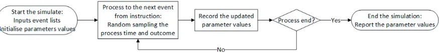
In this braking system repair process, the time resulting from the execution of the process can be evaluated using the Discrete Event Simulation (DES) technique. The overall steps of a DES program are illustrated in Figure 6.

Figure 6: Overall structure of a Discrete Event Simulation program

There are two main elements used to formulate a Discrete Event Simulation: variables and events. The variables are used to record system states and the time lapsed. Events are used to introduce the dynamics into the simulation and cause changes in the system states and therefore the variables. The DES approach is used to analyse systems where the variables change only at discrete points in time [9]. Generally, there are three types of variable used to govern the simulation process and collect information relating to the system performance [10]:

1. The time variables: to record the time lapsed, t.

2. Counter variables: to record the number of times that certain events have occurred by lapsed time t.

3. System states variables:to record the states of the system components and the system at lapsed time t.

When a simulation trial starts, an event list is generated which defines all events which can occur and the times, sampled from an appropriate distribution, at which they occur. The software will then identify the next event to occur and process it to determine what further events can happen as a result of it. The new events are added to the event list and again the next event to occur is identified. The process is continued recording the values of relevant variables as the simulation progresses. In order to keep a continuous record of the system evolution, variable values are cached whenever an event happens. A simulation trial finishes when a pre-defined system state is reached or when the system life duration is excessed. To get statistical significance in the performance predictions, many system trials have to be performed.

distribution of the process variables, the most significant of which is the expected maintenance process execution time, t. The process task completion time duration and outcome are generated stochastically and the process execution time is the accumulation of time durations of all executed tasks.

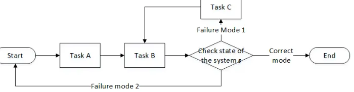
As a demonstration, consider an example process diagram shown in Figure 7. The FMEA table for the task events is given in Table VI. The process contains three tasks that are performed in sequence. Task A is conducted first, and then task B. As shown in Table VI, task A affects the state the of component s1, and has a 0.9 chance of transitioning the state of s1 from the default condition to the correct condition and a 0.1 probability that the state of s1 remains in its default. Task B affects the state of component s2 and has a 0.8 chance of transitioning the state of s2 from default to the correct condition and a 0.2 chance to an incorrect condition. A test is performed before termination to reveal the state of the system as determined by the conditions of its two components, s=(s1, s2). If both of the components are in their correct states, then the simulation is completed. If not and if s2 is in the wrong state (s is in failure mode 1), then task C is performed and task B is repeated; Otherwise for any other incorrect situation, the entire process is repeated from the start.

Figure 7: An example in order to illustrate the Discrete Event Simulation process

Each time a task is executed in the process, a probability and a time duration value are randomly generated to determine to which state the affected component will reside in after the task is completed and the duration that the task takes to compete. Consider for instance task A: a random value from 0 to 1, [0,1), is generated. If the value is smaller than 0.9, then the component will transfer to state of s1, otherwise if the value is in the range [0.9,1), then the state of s1 remains unchanged. If the state of s1 changes, then a time to complete the task is sampled from a normal distribution with mean 10s and standard deviation 1s and added into the overall process execution time, t; otherwise, no time is added. A simulation is completed when the “check state of system s” task executed before the process termination reveals the required system states, s=(s1=correct, s2=correct). The process execution time is then recorded so that an accurate estimate of the process completion time can be calculated once many simulations have been performed.

In the example braking system repair MP, the state transitions result from the execution of each process task (as given in Table I), which are performed in the order illustrated in Figure 2. Whenever an event has occurred, the values of the relevant performance variables may be changed and all the updated values recorded. The detailed description of all tasks (the prerequisite conditions, the affected component, the possible failures and corrective actions) is given by the FMEA analysis in Section 3. In this way the system status can be followed, as it evolves over time.

P(

|

_|

√

1 Task nam e 2 Input s 3 Outputs if the task is correctly performe d 4 Prerequisite Conditions (Requirements of hardware states) 5 Affect Component and its efficient initial state

6 The effect of task on the component 7 Local effect 8 Global effect Hardwar e Compon ent State Hardwar e Compon ent

State State Probabil

ity Time

Task A

n/a n/a n/a S1 default Correct 0.9 N(10,1

)

State of S1

is incorrect System _{state is} incorrect

Default 0.1 0

Task

B n/a n/a

S1 correct S2 default Correct 0.8 N(20.6

)

State of S2

is incorrect System _{state is} incorrect Incorre

ct 0.2 N(30,6)

Task

C n/a n/a n/a

S2 incorre

The following steps give detailed description of how to determine the stopping point of a simulation [10]:

1. Select an acceptable value d for the standard deviation of the estimator. 2. Simulate for at least 100 trials.

3. Carry on generating new trials data; stop when the number of total trials, n, satisfies 1.96S_n

√

4. The estimate of the population mean is given by _X´

n=

∑

n Xi

n .

In order to achieve a reliable process execution time for the braking system repair example, 95% confidence interval and d=60s has been used to determine the stopping criterion for estimating the average execution time for each of the braking system process design considered.

4.2 Process Design Optimisation

There are 20 tasks in the basic repair process for the car braking system repair example. Each task may be followed by a failure-detection action and corresponding corrective sequence. Therefore, there are 18 optional tests (C8 and C18 are compulsory tests) and will be 262144 possible process designs. Since it is too time consuming to explore all of these possible options in a realistic time, an optimisation routine is used to select the most effective failure detection tasks to incorporate. In this case, a genetic algorithm has been used to find the minimal time solution.

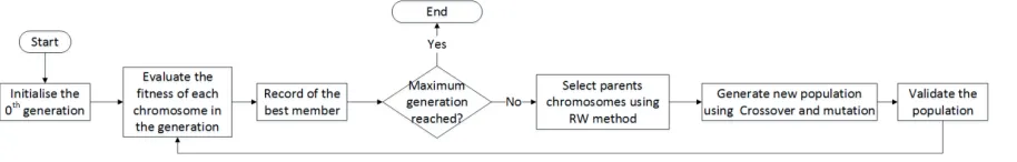
The Genetic Algorithm (GA): GAs were first proposed in as a means to find good solutions to problems that were otherwise computationally intractable [12]. Each GA operates on a population of artificial chromosomes, each of which represents a solution to a problem and has a fitness value. The fitness value is used to measure the goodness of the performance of the solution and is determined by simulating the design represented by the chromosome. A GA starts with a randomly generated population of chromosomes and then produces the next generation by applying selection, crossover, and mutation operators. Those chromosomes which represent good design options, as indicated by their fitness values, are selected to form the next generation of solutions. The selected parent chromosomes are recombined using crossover to produce child chromosomes, which are then used in the successor population. The mutation operator introduces a random diversity into the process to ensure that the full design space is explored and gives some confidence that the optimisation will produce a global rather than local optimal. This process is repeated over several iterations until some stopping criterion, such as the maximum number of generations, or convergence is reached. In this way, the GA will evolve to a ‘best’ solution to a given problem [4]. The steps of the GA used to choose the optimal combinations of tests to minimise the braking system repair process time are shown in Figure 8.

Figure 8: The overall structure of the GA program

Chromosome Design: A chromosome is a vector of Boolean variables which represent a potential solution to the problem. For example, there are 18 optional tests which can be included or excluded in any design option for the maintenance process. The inclusion of each test in the chromosome is represented by a gene. The location of a gene in the string is used to represent the test associated with the ith _{process task. The gene is represented as a Boolean} variable where a value of 1 is used to represent that the corresponding test is selected in the current repair process and a value of 0 to represent the absence of the corresponding test task. Consider the chromosome structure shown in Figure 9, the value of the first gene is 0, meaning that the test that reveals the successful completion of the first process task is not included in the solution. The value of the fourth gene is 1, meaning that the test that shows whether the fourth task is successful is included.

Figure 9: The chromosome structure encoding the inclusion information of all tests

Design Fitness Values: The fitness of a chromosome is a value that is used to determine the goodness of the design represented by the chromosome. For the example considered, the fitness value is determined by the overall execution time of a process design with the test list represented by a chromosome subtracted from a large-enough process execution times (2000s). Process designs with execution time larger than 2000s is given a fitness value of 0. Each chromosome produced by the GA gives a sequence of tests, which is then integrated in the standard repair process as shown in Figure 2 to form a specific process design. The execution time of the process design is then evaluated using the DES described in Section 4.1. The steps of evaluating the fitness of a chromosome are described below:

1. Obtain the test list using information from each chromosome in the GA.

2. Integrate the test list with the standard repair process to form the overall maintenance process design.

3. Use the DES to calculate the mean execution time for the process design.

Tournament and Truncation [13]. Here, the most common one is used: the Roulette Wheel method. Each chromosome is given a slice of a circular roulette wheel equal in area to the chromosome’s fitness and the slice where the randomly landing ball stopped is selected, meaning the probability that an individual is selected equals to its fitness divided by the total fitness of the population [14].

Crossover and Mutation: The selected, highly fit, chromosomes from the previous generation are then recombined (using crossover and mutation operations) to produce the chromosomes for the next generation. For each pair of chromosomes in a generation, a crossover rate is used to decide whether this pair will conduct the crossover operation to produce children chromosomes for the next generation. If so, for two parent chromosomes shown in Figure 10, the crossover operation starts with selecting an identical crossover point for them to divide each parent into part A and part B, and then combine part A/B of the first parent with the part B/A of the second parent to obtain two children chromosomes. For each child chromosome, the mutation operation changes its structure by transferring each gene from a value of 0 to 1 or vice versa with a specified mutation rate. Both crossover and mutation happen with a certain probability in reasonable ranges (from 0.6 to 9.0 for crossover rate and 0.01 to 0.05 per bit for the mutation rate [15]).

Figure 10: Illustration of crossover between two chromosomes and the mutation of gene in one chromosome

5

RESULTS AND DISCUSSION

5.1 The choice of GA parameters

An analysis was conducted to identify the effect of choices of initial population size, crossover rate and mutation rate on the optimal solution after 60 generation. From Figure 11 to Figure 13, it can be seen that the change of population size, crossover rate, and mutation rate will affect the ‘best’ solution that is obtained after the defined number of generations. Initially, the parameters were set to population size 20, crossover rate 0.8 and mutation rate 0.05. Considering first of all the impact of population size selected, retaining the values of the other parameters. The value of population size was varied from 10 to 40 and the results shown in Figure 11. This gives the following trends:

 When the population size is small, e.g. 10, the time of the best solution from the 1st generation to the 60th _{generation decrease only by a small margin. This means the GA} is not able to efficiently identify a best solution.

 With increasing population size, the time degree of improvement difference between the best solutions obtained at the beginning and at the end of the GA is greater.

is 30 and simulation time of 967s when the population size is 40. An optimal final solution can be obtained when the population size is 20.

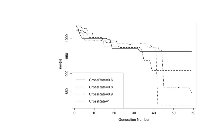
The investigation performed for the population size is applicable also to crossover rate and mutation rate. By changing the crossover rate (0.6 to 1) and mutation rate (0.01 to 0.05), the trends in the best value solutions with generation evolution are illustrated in Figure 12 and Figure 13 respectively.

After simulations using different values of GA parameters and comparing the performance under different parameters, an optimisation process was established using population size of 20, a crossover rate of 0.9 and a mutation rate of 0.03, as those parameter values tend to lead to the a better time solution.

Figure 11: The time of the best solution of each generation with a population size of 10, 20, 30 or 40 respectively

Figure 13: The time of the best solution of each generation with a mutation rate of 0.01, 0.03 or 0.05 respectively

5.2 Simulation Results

An optimal solution containing the best combination of failure tests in the overall maintenance process can be obtained using stated parameter values. The simulation results using the GA are illustrated in Figure 14 with some of the values shown in Table VII. Each dot represents the mean time of all solutions of each generation from 1 to 60 and the line shows the trend of the lowest time (the execution time of the best solution of each generation). We can see that after the 43th _{generation, the lowest execution time has become} stable and convergence is achieved.

Table VII: The mean execution time of process designs and the time of the optimal process design of each generation

Generation Number (th) 1 10 20 30 40 50 60

Mean time of the generation (s)

1161 1156 1128 1111 1084 1141 1071

Time of the optimal process design (s)

1038 995 988 986 975 811 811

Figure 14: The trend of simulation results (mean time of all solutions and the lowest time within all solutions in each generation) with the increasing of generation number.

C 1

C 2

C 3

C 4

C 5

C

6 C7 C8 C9 C1

0 C11 C1

2 C1

3 C1

4 C1

5 C1

6 C1

7 C1

8 C1

9 C2

0 0 0 0 1 1 1 0 1 0 0 0 0 0 1 1 0 1 1 0 0

Figure 15: Chromosome structure encoding the optimal tests selection

Integrating the selected test options, as given in Figure 2, we can obtain the optimal braking system repair process design, as shown in Figure 16.

Figure 16: The instruction of the braking system repair process with the optimal tests selection

The distribution of simulation results (process execution time) for the standard braking system repair process, for the optimal process design, and for two example non-optimal process designs, are illustrated in Figure 17. Each process designed was simulated for many trials until the stopping criteria described in Section 4.1.2 were met. The mean time for the optimal braking system repair process is 811s (simulation results distribution is shown in the top-right of Figure 17), which decreases significantly (36%) compared with the one for the standard process design without any optional tests (top-left of Figure 17), 1276s. Simulation results of two non-optimal process designs with mean execution time of 1038s and 975s are shown in the bottom-left and bottom-right of Figure 17 respectively (The process design for the bottom-left figure includes tests after task 2, 4, 8, 11, 14, and 18; the process design for the bottom-right figure includes tests after task 4, 6, 7, 8, 14, 15, 17 and 18).

restore the braking system functionality can be achieved. The results in this section show that the inclusion of effective tests can potentially significantly reduce MP time.

Figure 17: The histograms of execution times of the process design without any optional tests (as shown in Figure 2), the optimal process design, a non-optimal process design that has an average execution time of 1038s and 975s respectively.

5.3 Potential Application

maintenance procedure can be achieved. The maintenance time can also be accurately predicted, which can be used to assist the business to make decisions on the arrangement of their service lines.

6

CONCLUSIONS

In order to minimise the completion time of a maintenance process, the research presented in this paper has developed a framework to select tests to identify errors made whilst the maintenance is underway. The framework has three key elements: identification of the possible tests which can be performed, simulation of a maintenance process with the selected tests embedded to determine the time distribution for successful completion and finally an optimisation phase which enables the tests to be selected in order to perform the process in the shortest time. A modified FMEA has been used in the first of these phases to identify the potential tests, the completion time distribution for any maintenance process is evaluated using a discrete time simulation and a Genetic Algorithm is employed for the optimisation.

A simple car braking system has been used to demonstrate the application of the method. The method is generic in nature and due to the flexibility of the simulation process can be used to model any maintenance procedure from any industry. Clearly, minimising the maintenance duration, and therefore the unavailability of the system, is of interest in any industry and having the distribution of times to complete provides extra information and insight to what can be achieved including an appreciation of the worst and best times in addition to the average.

An example when knowing the distribution of maintenance completion times is valuable is when you have a set window of opportunity to carry through maintenance. At the end of the window the system has to be repaired, tested and functional. From the distribution of completion times it will be possible to understand the risk of not completing the work within the available time.

ACKNOWLEDGEMENTS

Dr Yang Zhang, Prof John Andrews and Dr Sean Reed gratefully acknowledge the contribution from the Faste Laboratory, Centre for Functional Product Innovation at Lulea University of Technology for the support of this project.

REFERENCE

[1] M. Löfstrand, P. Kyösti, S. Reed, and B. Backe, “Evaluating availability of functional products through simulation,” Simul. Model. Pract. Theory, vol. 47, pp. 196–209, 2014.

[2] Y. Zhang, S. Reed, J. D. Andrews, and M. Löfstrand, “Predicting the Optimal Testing Strategy for Maintenance Procedures,” in The 49th ESReDA Seminar, 2015, p. 8. [3] J. McCall, “Genetic algorithms for modelling and optimisation,” J. Comput. Appl.

[4] T. Alonso-Rasgado, G. Thompson, and B.-O. Elfström, “The design of functional (total care) products,” Journal of Engineering Design, vol. 15, no. 6. pp. 515–540, 2004. [5] “Antilock braking system,” Encyclopædia Britannica, Inc, 2016. [Online]. Available:

https://www.britannica.com/technology/antilock-braking-system.

[6] “Brake System,” RepairPal, 2016. [Online]. Available: http://repairpal.com/brakes. [Accessed: 09-Sep-2016].

[7] P. Kyösti, S. Reed, M. Lofstrand, J. D. Andrews, L. Karlsson, and S. Dunnett,

“Simulation of Industrial Support Systems in the Context of Functional Products,” in 19th Advanceds in Risk, Reliability and Technology Symposium, 2011, no. 2004, pp. 1– 5.

[8] Z. I. Botev, “The normal law under linear restrictions: simulation and estimation via minimax tilting,” J. R. Stat. Soc. Ser. B (Statistical Methodol., p. n/a--n/a, 2016. [9] J. Banks, J. Carson, B. L. Nelson, and D. Nicol, Discrete-Event System Simulation.

2004.

[10] R. Sheldon, Simulation, 2nd ed. Academic Press, 1997.

[11] L. Wasserman, All of statistics: a concise course in statistical inferences. Springer, 2011.

[12] J. H. Holland, Adaptation in Natural and Artificial Systems, vol. Ann Arbor. 1975. [13] T. Bäck, D. B. Fogel, and Z. Michalewicz, “Handbook of Evolutionary Computation,”

Evol. Comput., vol. 2, pp. 1–11, 1997.

[14] M. Melanie, An introduction to genetic algorithms, vol. 32, no. 6. 1996.

[15] D. Mora-Melia, P. L. Iglesias-Rey, F. J. Martinez-Solano, and V. S. Fuertes-Miquel, “Design of Water Distribution Networks using a Pseudo-Genetic Algorithm and Sensitivity of Genetic Operators,” Water Resour. Manag., vol. 27, no. 12, pp. 4149– 4162, 2013.

[16] P. O’Connor and A. Kleyner, Practical Reliability Engineering, 5th ed. John Wiley & Sons, Ltd, 2011.