Normalisation by evaluation for type theory, in type theory

NORMALISATION BY EVALUATION FOR TYPE THEORY, IN TYPE THEORY

THORSTEN ALTENKIRCH AND AMBRUS KAPOSI

School for Computer Science, University of Nottingham, Nottingham, United Kingdom e-mail address: [email protected]

Department of Programming Languages and Compilers, E¨otv¨os Lor´and University, Budapest, Hungary

e-mail address: [email protected]

Abstract. We develop normalisation by evaluation (NBE) for dependent types based on

presheaf categories. Our construction is formulated in the metalanguage of type theory using quotient inductive types. We use a typed presentation hence there are no preterms or realizers in our construction, and every construction respects the conversion relation. NBE for simple types uses a logical relation between the syntax and the presheaf interpretation. In our construction, we merge the presheaf interpretation and the logical relation into a proof-relevant logical predicate. We prove normalisation, completeness, stability and decidability of definitional equality. Most of the constructions were formalized in Agda.

1. Introduction

Normalisation by evaluation (NBE) is a technique to compute normal forms of typedλ-terms by evaluating them in an appropriate semantics. The idea was pioneered by Schwichtenberg and Berger [14], subsequently a categorical account using presheaf categories was given [8] and this approach was extended to System F [9, 10] and coproducts [7].

In the present paper we extend NBE to a basic type theory with dependent types which has Π-types and an uninterpreted family using a presheaf interpretation. We take advantage of our recent work on an intrinsic representation of type theory in type theory [13] which only defines typed objects avoiding any reference to untyped preterms or typing relations and which forms the basis of our formal development in Agda.

The present paper is an expanded version of our conference paper [12]. In particular we show here for the first time that our normalisation construction implies decidability of equality. This isn’t entirely obvious because our normal forms are indexed by contexts and types of which it is a priori not known wether equality is decidable. However, we observe that mimicking the bidirectional approach to type checking [17] we can actually decide equality

Key words and phrases: normalisation by evaluation, dependent types, internal type theory, logical relations, Agda.

This research was supported by EPSRC grant EP/M016951/1, USAF grant FA9550-16-1-0029 and COST Action EUTypes CA15123.

LOGICAL METHODS

l

c

Altenkirch and Kaposi

CC

of normal forms and hence, after combining it with normalisation, we obtain decidability for conversion.

1.1. Specifying normalisation. Normalisation can be given the following specification. We denote the type of well typed terms of typeA in context Γ byTmΓA. We are not interested in preterms, all of our constructions will be well-typed. In addition, this type is defined as a quotient inductive type (QIT, see [13]) which means that terms are quotiented with the conversion relation. It follows that on one hand if two terms t, t0 : TmΓA are convertible then they are equal: t≡TmΓAt0. On the other hand, the eliminator of TmΓA

ensures that every function defined from this type respects the conversion relation. This enforces a high level of abstraction when reasoning about the syntax: all of our constructions need to respect convertibility as well.

The type of normal forms is denoted NfΓAand there is an embedding from it to terms

p–q:NfΓA→TmΓA. Normal forms are defined as a usual inductive type (as opposed to quotient inductive types).

Normalisation is given by a function norm which takes a term to a normal form. It needs to be an isomorphism:

completeness norm↓ TmΓA

NfΓA ↑p–q stability

If we normalise a term, we obtain a term which is convertible to it: t ≡ _pnormtq. This is called completeness. The other direction is called stability: n≡normpnq. It expresses that there is no redundancy in the type of normal forms. Soundness, that is, if t≡t0 then normt≡normt0 is given by congruence of equality.

1.2. NBE for simple type theory. Normalisation by evaluation (NBE) is one way to implement this specification. It works by a complete model construction (figure 1). We define a model of the syntax and hence the eliminator gives us a function from the syntax to the model. Then we define a quote function which is a map from the model back to the syntax, but it targets normal forms (a subset of the syntax via the operator p–q).

Syntax _Model

Normal forms

eliminator

quote

Figure 1: Normalisation by evaluation.

denoted_JA_Kis aRENop→Setfunctor. Terms and substitutions are natural transformations between the corresponding presheaves, e.g. fort:TmΓA we have a natural transformation

JtK:JΓK→˙ JAK. A function type is interpreted as the presheaf exponential (a function for all future worlds), the base type is interpreted as normal forms of the base type.

Because REN has contexts as objects, we can embed types into presheaves (Yoneda embedding): a type A is embedded into the presheaf TMA by setting TMAΨ =TmΨAi.e.

a type at a given context is interpreted as the set of terms of that type in that context. Analogously, we can embed a typeA into the presheaveas of normal forms NFA and neutral

terms NEA. Normal forms are terms with no redexes (they include neutral terms) while

neutral terms are either variables or an eliminator applied to a neutral term.

The quote function is defined by induction on types as a natural transformationqA:

JAK→˙ NFA. Quote is defined mutually with unquote which maps neutral terms into semantic elements: uA:NEA→˙ JAK.

To normalise a term, we also need to define unquote for neutral substitutions (lists of neutral terms). Then we get normalisation by calling unquote on the identity neutral substitution, then interpreting the term at this semantic element and finally quoting.

normA(t:TmΓA) :NfΓA:=qA JtK(uΓid)

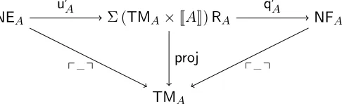
We can prove completeness using a logical relation R between TM and the presheaf model. The logical relation is equality at the base type. We extend quote and unquote to produce witnesses and require a witness of this logical relation, respectively. This is depicted in figure 2. The commutativity of the right hand triangle gives completeness: starting with a term, a semantic value and a witness that these are related, we get a normal form, and then if we embed it back into terms, we get a term equal to the one we started with.

Stability can be proven by mutual induction on terms and normal forms.

NEA Σ (TMA×JAK)RA NFA

TMA

u0_A q0_A

p–_q proj p–q

Figure 2: The type of quote and unquote for a type A in NBE for simple types. We use primed notations for the unquote and quote functions to denote that they include the completeness proof. This is a diagram in the category of presheaves.

A nice property of this normalisation proof is that the part of unquote (and quote) which gives (and uses) _JA_Kcan be defined separately from the part which gives relatedness. This means that the normalisation function can be defined independently from the proof that it is complete.

In the case of simple type theory, types are closed, so they are interpreted as presheaves just as contexts. When we have dependent types, types depend on contexts, hence they are interpreted as families of presheaves in the presheaf model (we omit functoriality).

JΓK :|REN| →Set

JΓ`AK: (Ψ :|REN|)→JΓKΨ→Set

We can declare quote for contexts the same way as for simple types, but quote for types has to be more subtle. Our first candidate is the following where it depends on quote for contexts (we omit the naturality properties).

qΓ : (Ψ :|REN|)→_JΓ_KΨ→TmsΨ Γ

qΓ`A: (Ψ :|REN|)(α:JΓKΨ)→JAKΨα→NfΨ A[qΓ,Ψα]

The type of unquote also depends on quote for contexts.

uΓ`A: (Ψ :|REN|)(α :JΓKΨ)→NeΨ A[qΓ,Ψα]

→_JA_KΨα

When we try to define quote and unquote following this specification, we observe that we need some new equations to typecheck our definition. E.g. quote for function types needs that quote after unquote is the identity up to embedding: p–q◦qA ◦uA ≡p–q. This is

however the consequence of the logical relation between the syntax and the presheaf model: we can read it off figure 2 by the commutativity of the diagram: if we embed a neutral term into terms, it is the same as unquoting, then quoting, then embedding.

Hence, our second attempt is defining quote and unquote mutually with their correctness proofs. It is not very surprising that when moving to dependent types the well-typedness of normalisation depends on completeness. The types of quote and unquote become the following.

qΓ`A: (Ψ :|REN|)(ρ:TmsΨ Γ)(α :JΓKΨ)(p:RΓ Ψρ α)

(t:TmΨA[ρ])(v:JAKΨα)→RAΨpt v→Σ(n:NFAρ).t≡pnq

uΓ`A Ψρ α p: (n:NeΨA[ρ])→Σ(v:JAKΨα).RAΨppnqv

However there seems to be no way to define quote and unquote this way because quote does not preserve the logical relation. The problem is that when defining unquote at Π we need to define a semantic function which works for arbitrary inputs, not only those which are related to a term. The first component of unquote at Π has the following type.

proj₁

uΓ`ΠA BΨρ α p n:NeΨ (ΠA B)[ρ]

:∀Ω.(β:REN(Ω,Ψ)) x:_JA_KΩ(JΓKβ α)

→_JB_KΩ(JΓKβ α, x)

We should define this as unquoting the application of the neutral functionn and quoting the inputx. However we can’t quote an arbitrary semanticx, we also need a witness that it is related to a term. It seems that we have to restrict the presheaf model to only contain semantic elements which are related to some term.

Indeed, this is our solution: we merge the presheaf model and the logical relation into a single proof-relevant logical predicate. We denote the logical predicate at a context Γ by PΓ. We define normalisation following the diagram in figure 3.

NEΓ ΣTMΓPΓ NFΓ

TMΓ

uΓ qΓ

p–q proj p–q

Figure 3: The types of quote and unquote for a context Γ in our proof.

form which is equal to the term (this is why it needs to be proof-relevant). This solves the problem mentioned before: now the semantics of a term will be the same term together with a witness of the predicate for that term.

1.4. Structure of the proof and the paper. In this subsection, we give a high level sketch of the proof. Sections 3, 4, 5, 7 are fully formalised in Agda, the computational parts of sections 6, 8 and 9 are formalised, but some of the naturality and functoriality properties are left as holes. The formalisation is available online [11]. The proofs are available in full detail on paper (including everything that we omitted in this paper and which is not finished in the formalisation) in the second author’s thesis [25].

In section 2 we briefly summarize the metatheory we are working in.

In section 3 we define the syntax for type theory as a quotient inductive inductive type (QIIT) [13]. The arguments of the eliminator for the QIIT form a model of type theory.

In section 4 we prove injectivity of context extension and the type formers Eland Π. We will need these for proving decidability of equality for normal forms.

In section 5 we define the category of renamingsREN: objects are contexts and morphisms are renamings.

In section 6 we define the proof-relevant presheaf logical predicate interpretation of the syntax. The interpretation has RENas the base category and two parameters for the interpretations ofU andEl. This interpretation can be seen as a dependent version of the presheaf model of type theory. E.g. a context in the presheaf model is interpreted as a presheaf. Now it is a family of presheaves dependent on a substitution into that context. The interpretations of base types can depend on the actual elements of the base types. The interpretation of substitutions and terms are what are usually called fundamental theorems.

In section 7 we define neutral terms and normal forms together with their renamings and embeddings into the syntax (p–q). With the help of these, we define the interpretations of U andEl. The interpretation ofU at a term of typeU will be a neutral term of typeU which is equal to the term. We also prove decidability of equality for normal forms.

In section 8 we mutually define the natural transformations quote and unquote. We define them by induction on contexts and types as shown in figure 3. Quote takes a term and a semantic value at that term into a normal term and a proof that the normal term is equal to it. Unquote takes a neutral term into a semantic value at the neutral term.

1.5. Related work. Normalisation by evaluation was first formulated by Schwichtenberg and Berger [14], subsequently a categorical account using presheaf categories was given [8] and this approach was extended to System F [9, 10] and coproducts [7]. The present work can be seen as a continuation of this line of research. A fully detailed description of our proof can be found in the PhD thesis of the second author [25].

The term normalisation by evaluation is also more generally used to describe semantic based normalisation functions. E.g. Danvy is using semantic normalisation for partial evaluation [20]. Normalisation by evaluation using untyped realizers has been applied to dependent types by Abel et al. [2–4]. Danielsson [19] has formalized NBE for dependent types but he doesn’t prove soundness of normalisation.

Our proof of injectivity of type formers is reminiscent in [22] and the proof of decidability of normal forms is similar to that of [5].

2. Metatheory and notation

We are working in intensional Martin-L¨of Type Theory with postulated extensionality principles using Agda as a vehicle [1, 27]. We make use of quotient inductive inductive types (QIITs, see section 6 of [13]). QIITs are a combiniation of inductive inductive types [26] and higher inductive types [29]. The metatheory of QIITs is not developed yet, however we hope that they can be justified by a setoid model [6]. We only use one instance of a QIIT, the definition of the syntax. We extend Agda with this QIIT using axioms and rewrite rules [15]. The usage of rewrite rules guarrantees that injectivity and disjointness of constructors of the QIIT are not available to the unification mechanisms of Agda. Also, pattern matching on constructors of the QIIT is not available, the only way to define a function from the QIIT is to use the eliminator.

When defining an inductive typeA, we first declare the type bydataA:S whereS is the sort, then we list the constructors. For inductive inductive types we first declare all the types, then following a seconddata keyword we list the constructors. We also postulate functional extensionality which is a consequence of having an interval QIIT anyway. We assume K, that is, we work in a strict type theory.

We follow Agda’s convention of denoting the universe of types bySet, we write function types as (x:A)→B or∀x.B, implicit arguments are written in curly braces {x:A} →B and can be omitted or given in curly braces or lower index. If some arguments are omitted, we assume universal quantification, e.g. (y:B x) →C means ∀x.(y:B x)→C ifx is not given in the context. We write Σ(x:A).B for Σ types. We overload names e.g. the action on objects and morphisms of a functor is denoted by the same symbol.

The identity type (propositional equality) is denoted – ≡ – and its constructor is refl. Transport of a term u :P a along an equality p : a ≡ a0 is denoted p∗u : P a0. We

denote (p∗u) ≡ u0 by u ≡p u0. We write ap for congruence, that is apf p : f a ≡ f a0 if

p:a≡a0. We write – – for transitivity and –−1 _{for symmetry of equality. For readability,} we will omit writing transports in the informal presentation most of the time, that is, our informal notation is that of extensional type theory. This choice is justified by the conservativity of extensional type theory over intensional type theory with K and functional extensionality [23, 28]. This allows writing e.g.f a wheref :A→B anda:A0 in case there is an equality in scope which justifiesA≡A0.

underscore to denote arguments that we don’t need e.g. the constant function is written constx :=x.

3. Object theory

The object theory is a basic type theory with dependent function space, an uninterpreted base typeUand an uninterpreted family over this base typeEl. We use intrinsic typing (that is, we only define well typed terms, term formers and derivation rules are indentified), and we present the theory as a QIIT, that is, we add conversion rules as equality constructors. We define an explicit substitution calculus, hence substitutions are part of the syntax and the syntax is purely inductive (as opposed to inductive recursive). For a more detailed presentation, see [25].

The syntax constitutes of contexts, types, substitutions and terms. We declare the QIIT of the syntax as follows.

data Con :Set

data Ty :Con→Set

data Tms:Con→Con→Set

data Tm : (Γ :Con)→TyΓ→Set

We use the convention of naming contexts Γ,∆,Θ, types A, B, terms t, u, substitutions σ, ν, δ.

The point constructors are listed in the left column and the equality constructors in the right.

data data

· :Con [id] :A[id]≡A

–,– : (Γ :Con)→TyΓ→Con [][] :A[σ][ν]≡A[σ◦ν]

– [ – ] :Ty∆→TmsΓ ∆→TyΓ U[] :U[σ]≡U

U :TyΓ El[] : (ElAˆ)[σ]≡El(U[]∗Aˆ[σ])

El :TmΓU→TyΓ Π[] : (ΠA B)[σ]≡Π (A[σ]) (B[σ ↑A])

Π : (A:TyΓ)→Ty(Γ, A)→TyΓ id◦ :id◦σ ≡σ

id :TmsΓ Γ ◦id :σ◦id≡σ

–◦– :TmsΘ ∆→TmsΓ Θ→TmsΓ ∆ ◦◦ : (σ◦ν)◦δ ≡σ◦(ν◦δ)

:TmsΓ· η :{σ:TmsΓ·} →σ≡

–,– : (σ:TmsΓ ∆)→TmΓA[σ]→TmsΓ (∆, A) π1β :π1(σ, t)≡σ

π1 :TmsΓ (∆, A)→TmsΓ ∆ πη : (π1σ, π2σ)≡σ

– [ – ] :Tm∆A→(σ:TmsΓ ∆)→TmΓA[σ] ,◦ : (σ, t)◦ν ≡(σ◦ν),(_[][]∗t[ν])

π2 : (σ:TmsΓ (∆, A))→TmΓA[π1σ] π2β :π2(σ, t)≡π1β t

lam :Tm(Γ, A)B→TmΓ (ΠA B) Πβ :app(lamt)≡t

app :TmΓ (ΠA B)→Tm(Γ, A)B Πη :lam(appt)≡t

lam[] : (lamt)[σ]≡Π[]_{lam(t[σ ↑A])}

• Substitutions form a category with a terminal object. This includes the categorical substitution laws for types [id] and [][].

• Substitution laws for typesU[],El[], Π[].

• The laws of comprehension which state that we have the natural isomorphism

π1β, π2β –,– ↓ σ :TmsΓ ∆ TmΓA[σ]

TmsΓ (∆, A) ↑π1, π2 πη

where naturality1 is given by ,◦.

• The laws for function space which are given by the natural isomorphism

Πβ lam↓ Tm(Γ, A)B

TmΓ (ΠA B) ↑app Πη

where naturality is given by lam[].

Note that the equalityπ2β lives over π1β. Also, we had to use transport to typecheck El[] and,◦. We used lifting of a substitution in the types of Π[] andlam[]. It is defined as follows.

– ↑ – : (σ:TmsΓ ∆)→Ty∆→Tms(Γ, A[σ]) (∆, A)

σ ↑A:= (σ◦π1id),([][]∗π2id)

We use the categorical appoperator but the usual one ( – $ – ) can also be derived.

h(u:TmΓA)i :TmsΓ (Γ, A) :=id,[id]−1_∗u

(t:TmΓ (ΠA B))$(u:TmΓA) :B[hui] := (appt)[hui]

When we define a function from the above syntax, we need to use the eliminator. The eliminator has four motives corresponding to what Con,Ty,Tms andTm get mapped to and one method for each constructor including the equality constructors. The methods for point constructors are the elements of the motives to which the constructor is mapped. The methods for the equality constructors demonstrate soundness, that is, the semantic constructions respect the syntactic equalities. The eliminator comes in two different flavours: the non-dependent and dependent version. In our constructions we use the dependent version. The motives and methods for the non-dependent eliminator (recursor) collected together form a model of type theory, they are equivalent to Dybjer’s Categories with Families [21].

To give an idea of what the eliminator looks like we list its motives and some of its methods. For a complete presentation and an algorithm for deriving these from the constructors, see [25]. As names we use the names of the constructors followed by an upper

1_{If one direction of an isomorphism is natural, so is the other. This is why it is enough to state naturality}

indexM.

ConM :Con→Set

TyM : (ConMΓ)→TyΓ→Set

TmsM : (ConMΓ)→(ConM∆)→TmsΓ ∆→Set

TmM : (ΓM:ConMΓ)→TyMΓMA→TmΓA→Set

·M _:ConM_·

–,M– : (ΓM:ConMΓ)→TyMΓMA→ConM(Γ, A)

idM :TmsMΓMΓMid

–◦M _{– :Tms}M_ΘM_∆M_σ→TmsM_ΓM_ΘM_{ν →Tms}M_ΓM_∆M_(σ◦ν)

◦idM :σM◦M_idM_≡◦id_σM

π2βM :πM2 (ρM,MtM)≡π1β M_,π

2β _tM

Note that the method equality◦idM lives over the constructor◦idwhile the method equality π2βM lives both over the method equalityπ1βM and the equality constructor π2β.

There are four eliminators for the four constituent types. These are understood in the presence of all the motives and methods given above.

ElimCon : (Γ :Con) →ConMΓ

ElimTy : (A:TyΓ) →TyM(ElimConΓ)A

ElimTms: (σ:TmsΓ ∆)→TmsM(ElimConΓ) (ElimCon∆)σ

ElimTm : (t:TmΓA) →TmM(ElimConΓ) (ElimTyA)t

We have the usual β computation rules such as the following.

ElimCon(Γ, A) =ElimConΓ,MElimTyA

ElimTms(σ◦ν) =ElimTmsσ◦MElimTmsν

There are no β rules for the equality constructors (such rules would be only interesting in a setting without K).

4. Injectivity of context and type formers

As examples of using the eliminator we prove injectivity of context and type constructors. We will need these results when proving decidability of equality for normal forms in section 7.

First, given Γ0 :Con and A0 :TyΓ0 we define a family over contexts P : Con → Set using the eliminator. We specify the motives and methods as follows.

ConM :=Set

TyM :=>

TmsM :=>

TmM :=>

·M :=⊥

–,M–{Γ :Con} {A:TyΓ} := Σ(q : Γ0 ≡Γ).A0 ≡qA

idM, ... :=tt

◦idM, ... :=refl

A context is interpreted as a type. Types, substitutions and terms are interpreted as elements of the unit type, hence the interpretations of all the type formers, substitution and term constructors are triviallyttand all the equalities hold by reflexivity. The empty context is interpreted as the empty type (we will never need this later) and an extended context (Γ, A) is interpreted as a pair of equalities between Γ0 and Γ andA0 andA (the latter depends on the former equality). When defining –,M– we wrote underscores for the interpretations of Γ andA (having typesSetand>, respectively) thus ignoring these arguments, we only used Γ and Athemselves which are implicit arguments of the eliminator. Using the above motives and methods, we define P:=ElimCon:Con→Set and theβ rule tells us that

P(Γ0, A0) = Σ(q: Γ0≡Γ0).A0 ≡q A0

and

P(Γ1, A1) = Σ(q: Γ0 ≡Γ1).A0≡qA1.

We can prove the first one by (refl,refl) and given an equality wbetween the indices (Γ0, A0) and (Γ1, A1), we can transport it to the second one. This proves injectivity:

inj,: w: (Γ0, A0)≡(Γ1, A1):=w∗(refl,refl) : Σ(q : Γ0 ≡Γ1).A0≡qA1

To show injectivity of type formers, we start by the definition of normal types. These are eitherU,Elor Π, but not substituted types. Then we show normalisation of types using the eliminator (this just means pushing down the substitutions until we reach a U orEl). Finally we prove the first injectivity lemma for Π using normalisation.

constructor names.

data NTy: (Γ :Con)→Set

p–q :NTyΓ→TyΓ data NTy

U :NTyΓ

El :TmΓU→NTyΓ

Π : (A:NTyΓ)→NTy(Γ,pAq)→NTyΓ

pΠA Bq := ΠpAq pBq

pUq :=U

pElAˆq :=ElAˆ

Substitution of normal types can be defined by ignoring the substitution for U, applying it to the term for Eland substituting recursively for Π. We need to mutually prove a lemma saying that the embedding is compatible with substitution. AsNTyis a simple inductive type (no equality constructors) we use pattern matching notation when defining these functions.

– [ – ] :NTy∆→TmsΓ ∆→NTyΓ

p[]q : (A:NTy∆)(σ :TmsΓ ∆)→_pAq[σ]≡_pA[σ]q

(ΠA B)[σ] := Π (A[σ]) (B[(p[]qA σ)∗σ↑A])

U[σ] :=U

(ElAˆ)[σ] :=El( ˆA[σ])

p[]q(ΠA B)σ := Π[]apΠ p[]qA σ

p[]qB(σ↑A) p[]qUσ :=U[]

p[]q(ElAˆ)σ :=El[]

When defining substitution of Π, we need to use p[]q to transport the lifted substitution σ ↑A to the expected type. The lemma p[]q is proved using the substitution laws of the syntax and the induction hypothesis in the case of Π. apΠ denotes the congruence rule for Π, its type is (pA:A≡A0)→B ≡pA B0→ΠA B ≡ΠA0B0.

By induction on normal types, we prove the following two lemmas as well.

[id] : (A:NTyΓ)→A[id]≡A

[][] : (A:NTyΓ).∀σ ν.A[σ][ν]≡A[σ◦ν]

Now we can define the model of normal types using the following motives for the eliminator.

ConM :=>

TyM{Γ} A:= Σ(A0:NTyΓ).A≡_pA0q

TmsM :=>

TmM :=>

to the trivial type. Hence, the methods for contexts, substitutions and terms will be all trivial and the equality methods for them can be proven byrefl.

The methods for types are given as follows.

– [ – ]M{A}(A0, pA){σ} := A0[σ],ap( – [σ])pA p[]qA0σ

UM := (U,refl)

ElM{Aˆ} := (ElA,ˆ refl)

ΠM{A}(A0, pA){B}(B0, pB) := ΠA0(pA∗B

0_),apΠp

ApB

– [ – ]M receives a type A as an implicit argument, a normal type A0 and a proofpA that

they are equal, a substitution σ as an implicit argument and the semantic version of the substitution which does not carry information. We use the above defined – [ – ] for substitutingA0 and we need the concatenation of the equalities pA and p[]q to provide the

equalitypA0[σ]q≡pA[σ]q. MappingU andElAˆto normal types is trivial, while in the case of ΠA B we use the inductive hypotheses A0 andB0 to construct ΠA0B0, and in a similar way we use pA and pB to construct the equality.

When proving the equality methods [id]M,[][]M,U[]M,El[]M and Π[]M, it is enough to show that the first components of the pairs (the normal types) are equal, thepAproofs will

be equal by K. The equality methods [id]M and [][]M are given by the above lemmas [id] and [][]. The semantic counterparts of the substitution lawsU[] and El[] are trivial, while Π[]M is given by a straightforward induction.

Using the eliminator, we define normalisation of types as follows.

norm(A:TyΓ) :NTyΓ :=proj₁(ElimTyA)

We can also show completeness and stability of normalisation (see section 1.1 for this nomenclature).

compl(A:TyΓ) :A≡_pnormAq:=proj₂(ElimTyA)

stab(A0 :NTyΓ) :A0≡normpAq

Stability is proven by a straightforward induction on normal types.

Injectivity of ΠNTy (the Π constructor for normal types) is proven the same way as we did for context extension: the family P can be simply given by pattern matching as NTy doesn’t have equality constructors. Given a typeA0, we define P as follows.

P:NTyΓ→Set

P(ΠNTyA B) :=A0 ≡A

PX:=⊥

Note that we can’t define the same family over Ty (using the eliminator of the syntax) because it does not respect the equality Π[]. With the help of this P, we can prove injectivity by transporting the reflexivity proof ofP(ΠNTy_A

0B0) = (A0 ≡A0) to that of P(ΠNTyA1B1) = (A0 ≡A1).

injΠNTy(w: ΠNTyA0B0≡ΠNTyA1B1) :A0 ≡A1 :=w∗refl

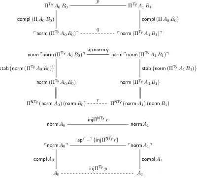
using stability we get r :norm(ΠTyA0B0) ≡norm(ΠTyA1B1). The type of r reduces to ΠNTy(normA0) (normB0)≡ΠNTy(normA1) (normB1) and now we can apply the injectivity of normal Π to get that normA0≡normA1. As a last step we apply p–q to both sides of this equality and use completeness onA0 and A1 to obtain A0 ≡A1.

ΠTyA0B0 ΠTyA1B1

p

pnorm(ΠTyA0B0)q pnorm(ΠTyA1B1)q

compl(ΠA0B0) compl(ΠA0B0)

q

normpnorm(ΠTyA0B0)q normpnorm(ΠTyA1B1)q ap normq

norm(ΠTyA0B0) norm(ΠTyA1B1)

stab norm(ΠTyA0B0)

stab norm(ΠTyA1B1)

ΠNTy(normA0) (normB0) ΠNTy(normA1) (normB1) r

normA0 normA1

injΠNTyr

pnormA0q pnormA1q

app–q injΠNTyr

A0 A1

complA0 complA1

injΠTyp

Figure 4: Proof of injectivity of ΠTy in the domain. The dashed lines are given by the fillers of the squares. The double lines are definitional equalities.

We only state the other two injectivity lemmas, they can be proved analogously to injΠTy.

injΠTy0: (w: ΠTyA0B0 ≡ΠTyA1B1)→B0≡injΠTywB1

injEl :ElTyAˆ0 ≡ElTyAˆ1 →Aˆ0 ≡Aˆ1

5. The category of renamings

In this section we define the category of renamings REN. Objects in this category are contexts, morphisms are renamings of variables (Vars).

We define typed De Bruijn variablesVar and renamingsVarstogether with their embed-dings into substitutions.

data Var : (Ψ :Con)→TyΨ→Set

vze :Var(Ψ, A) (A[π1id])

vsu :VarΨA→Var(Ψ, B) (A[π1id])

p–q :VarsΩ Ψ→TmsΩ Ψ data Vars:Con→Con→Set

:VarsΨ·

–,– : (β :VarsΩ Ψ)→VarΩA[pβq]→VarsΩ (Ψ, A)

p–q :VarΨA→TmΨA

pvzeq :=π2id

pvsuxq :=pxq[π1id]

pq :=

pβ, xq :=pβq,pxq

Variables are typed de Bruijn indices. vze projects out the last element of the context,vsu extends the context, and the type A:TyΨ needs to be weakened in both cases because we need to interpret it in Ψ extended by another type. Renamings are lists of variables with the appropriate types. Embedding of variables into terms uses the projections and the identity substitution, and embedding renamings is pointwise.

We use the names Ψ,Ω,Ξ for objects ofREN,x, yfor variables, β, γ for renamings. We need identity and composition of renamings for the categorical structure. To define them, we also need weakening and renaming of variables together with laws relating their embeddings to terms. We only list the types as the definitions are straightforward inductions.

wkV :VarsΩ Ψ→Vars(Ω, A) Ψ pwkVq:pβq◦π1id≡_pwkVβq

id :VarsΨ Ψ pidq :pidq≡id

–◦ – :VarsΞ Ψ→VarsΩ Ξ→VarsΩ Ψ p◦_q :pβq◦_pγq≡_pβ◦γq

– [ – ] :VarΨA→(β :VarsΩ Ψ)→VarΩA[pβq] p[]q :pxq[pβq]≡_px[β]q

Renamings form a category, we omit the statement and proofs of the categorical laws.

6. The logical predicate interpretation

We start by defining the Yoneda embedding TM which embeds a context into the sets of substitutions into that context, a type into the sets of terms into that context, and substitutions and terms into maps between the corresponding sets. We denote contravariant presheaves overC by PShC, families of presheaves over a presheaf byFamPShand natural transformations and sections by ˙→ and→s , respectively. See appendix A for the definitions of these categorical notions.

∆ :Con TM∆:PSh REN TM∆Ψ :=TmsΨ ∆ TM∆β ρ:=ρ◦pβq

A:TyΓ TMA :FamPSh TMΓ TMAΨρ:=TmΨA[ρ] TMAβ t :=t[pβq]

σ :TmsΓ ∆ TMσ :TMΓ→˙ TM∆ TMσΨρ :=σ◦ρ

t:TmΓA TMt :TMΓ

s

→TMA TMtΨρ :=t[ρ]

TM∆ is a presheaf over REN. The functor laws hold asρ◦_pidq≡ρ and (ρ◦_pβq)◦_pγq≡

ρ◦_pβ◦γq. TMA is a family of presheaves overTMΓ, and similarly we have t[pidq]≡t and t[pβq][pγq]≡t[pβ◦γq]. TMσ is a natural transformation, naturality is given by associativity:

(σ◦ ρ)◦ _pβq ≡ σ ◦(ρ◦_pβq). TMt is a section, it is naturality law can be verified as

t[ρ][pβq]≡t[ρ◦_pβq]. TM can be seen as a (weak) morphism in the category of models of type theory from the syntax into the presheaf model.

The motives for the presheaf logical predicate interpretation are given as families over the Yoneda embeddingTM. In contrast with section 4, here we use a recursive notation for defining the motives and methods.2

∆ :Con P∆:FamPSh TM∆

A :TyΓ PA :FamPSh Σ (ΣTMΓTMA)PΓ[wk]

σ :TmsΓ ∆ Pσ : ΣTMΓPΓ s

→P∆[TMσ][wk]

t :TmΓA Pt : ΣTMΓPΓ

s

→PA[TMt↑PΓ]

Note that – [ – ] above is the composition of a family of presheaves with a natural transfor-mation, wkis the weakening natural transformation and – ↑ – is lifting of a section (see appendix A for details).

We unfold these definitions below following appendix A.

A context ∆ is mapped to a family of presheaves over TM∆. That is, for every substitution ρ :TM∆Ψ we have a type P∆Ψρ expressing that the logical predicate holds for ρ. Moreover, we have the renaming P∆β :P∆Ψρ→P∆Ω(TM∆β ρ) for aβ :REN(Ω,Ψ). Sometimes we omit the parameter Ψ, also for theP operations on types, substitutions and terms.

PA is the logical predicate at a type A. It depends on a substitution (for which the

predicate needs to hold as well) and a term. PAΨ(ρ, s, α) expresses that the logical predicate

2_{For reference, the “arguments for the eliminator” notation for the motives looks as follows.}

ConM∆ :=FamPSh TM∆

TyMΓMA :=FamPSh Σ (ΣTMΓTMA) ΓM[wk]

TmsMΓM∆Mσ:= ΣTMΓΓM s

→∆M[TMσ][wk]

TmMΓMAMt := ΣTMΓΓM s

holds for terms:TmΨA[ρ].

A:TyΓ Ψ :|REN| ρ:TMΓΨ s:TMAρ α:PΓΨρ

PAΨ(ρ, s, α) :Set

It is also stable under renamings. That is, for aβ :REN(Ω,Ψ) we have

PAβ :PAΨ(ρ, s, α)→PAΩ(TMΓβ ρ,TMAβ s,PΓβ α).

A substitution σ is mapped to Pσ which expresses the fundamental theorem of the

logical predicate at σ: for any other substitutionρ for which the predicate holds, we can compose it with σ and the predicate will hold for the composition.

σ :TmsΓ ∆ Ψ :|REN| ρ:TMΓΨ α:PΓΨρ PσΨ(ρ, α) :P∆Ψ(σ◦ρ)

The fundamental theorem is also natural.

P∆β(PσΨ(ρ, α))≡PσΩ(TMΓβ ρ,PΓβ α)

A termtis mapped to the fundamental theorem at the term: given a substitution ρ for which the predicate holds, it also holds for t[ρ] in a natural way.

t:TmΓA Ψ :|RENop| ρ:TMΓΨ α:PΓΨρ PtΨ(ρ, α) :PAΨ(ρ, t[ρ], α)

PAβ PtΨ(ρ, α)

≡PtΩ(TMΓβ ρ,PΓβ α)

We define the presheafTMU:PSh RENand a family over itTMEl:FamPSh TMU. The actions on objects are TMUΨ := TmΨU and TMElΨAˆ:= TmΨ (ElAˆ). The action on a morphism β is just substitution – [pβq] for both.

Note that the base category of the logical predicate interpretation is fixed to REN. However we parameterise the interpretation by the predicate at the base type U and base familyEl. These are denoted by ¯Uand ¯Eland have the following types.

¯

U :FamPSh TMU

¯

El:FamPSh Σ (ΣTMUTMEl) ¯U[wk]

Now we list the methods for each constructor in the same order as we have given them in section 3. We omit the proofs of functoriality/naturality only for reasons of space (for these details see [25]).

The logical predicate trivially holds at the empty context, and it holds at an extended context forρif it holds at the smaller context atπ1ρand if it holds at the type which extends the context forπ2ρ. The second part obviously depends on the first. The action on morphisms for context extension is pointwise. Here we omitted some usages of –∗– e.g.P∆β α is only

well-typed in that position when we transport along the equality π1ρ◦pβq≡π1(ρ◦pβq). From now on we will omit transports and the usages of p–q in most cases for readability.

P·(ρ:TM·Ψ) :=>

P·β :=tt

P∆,A(ρ:TM∆,AΨ) := Σ(α:P∆(π1ρ)).PA(π1ρ, π2ρ, α)

P∆,A(β :REN(Ω,Ψ)) (α, a) := (P∆β α,PAβ a)

the substitution. Renaming a substituted type is the same as renaming in the original type (hence the functor laws hold immediately by the inductive hypothesis). This is well-typed

because of naturality ofTMσ andPσ as shown below.

P_A[σ](ρ, s, α) :=PA TMσρ, s,Pσ(ρ, α)

P_A[σ]β a :=PAβ a:PA TM∆β(TMσρ),TMAβ s,P∆β(Pσ(ρ, α))

| {z }

≡PA TMσ(TMΓβ ρ),TMAβ s,Pσ(TMΓβ ρ,PΓβ α)

The logical predicate at the base type and family says what we have given as parameters. Renaming also comes from these parameters.

PU(ρ, s, α) := ¯U(U[]∗s) PUβ a := ¯Uβ a

P_ElAˆ(ρ, s, α) := ¯El (El[]∗TM_Aˆρ), s,P_Aˆ(ρ, α)

P_ElAˆβ a:= ¯Elβ a

The logical predicate holds for a function swhen we have that if the predicate holds for an argument u (atA, witnessed by v), so it holds fors$u at B. In addition, we have a Kripke style generalisation: this should be true for TMΠA Bβ sfor any morphism β in a natural

way. Renaming a witness of the logical predicate at the function type is postcomposing the Kripke morphism by it.

PΠA BΨ (ρ:TMΓΨ),(s:TMΠA Bρ),(α:PΓρ)

:= Σ

map: β:REN(Ω,Ψ) u:TMA(TMΓβ ρ)

v:PAΩ(TMΓβ ρ, u,PΓβ α)

→PBΩ (TMΓβ ρ, u),(TMΠA Bβ s)$u,(PΓβ α, v)

.∀β, u, v, γ.PBγ(mapβ u v)≡map(β◦γ) (TMAγ u) (PAγ v)

PΠA Bβ0(map,nat) :=λβ.map(β0◦β), λβ.nat(β0◦β)

Now we list the methods for the substitution constructors, that is, we prove the fun-damental theorem for substitutions. We omit the naturality proofs. The object theoretic constructs map to their metatheoretic counterparts: identity becomes identity, composi-tion becomes composicomposi-tion, the empty substitucomposi-tion becomes the element of the unit type, substitution extension becomes pairing, first projection becomes first projection.

Pid(ρ, α) :=α

Pσ◦ν(ρ, α) :=Pσ TMνρ,Pν(ρ, α)

P(ρ, α) :=tt

Pσ,t(ρ, α) :=Pσ(ρ, α),Pt(ρ, α)

Pπ1σ(ρ, α) :=proj1 Pσ(ρ, α)

The fundamental theorem for substituted terms and the second projection are again just composition and second projection.

P_t[σ](ρ, α) :=Pt(TMσρ,Pσ(ρ, α))

Pπ2σ(ρ, α) :=proj2 Pσ(ρ, α)

witness of the predicate α to account for the Kripke property. The naturality is given by the naturality of the term itself.

Plamt(ρ, α) :=

λβ u v.Pt (TMΓβ ρ, u),(PΓβ α, v)

, λβ u v γ.natS Pt (TMΓβ ρ, u),(PΓβ α, v)

γ

Application uses the map part of the logical predicate and the identity renaming.

Pappt(ρ, α) :=map Pt(π1ρ,proj1α)

id(π2ρ) (proj2α)

Lastly, we need to provide methods for the equality constructors. We won’t list all of these proofs as they are quite straightforward, but as examples we show the semantic versions of the laws [][] and π2β. For [][], we have to show that the two families of presheavesPA[σ][ν] and PA[σ◦ν] are equal. It is enough to show that their action on objects and morphisms coincides as the equalities will be equal by K. Note that we use function extensionality to show the equality of the presheaves from the pointwise equality of actions. When we unfold the definitions for the actions on objects we see that the results are equal by associativity.

P_A[σ][ν](ρ, s, α)

=PA[σ] TMνρ, s,Pν(ρ, α)

=PA TMσ(TMνρ), s,Pσ(TMνρ,Pν(ρ, α))

≡PA TMσ◦νρ, s,Pσ(TMνρ,Pν(ρ, α))

=PA TMσ◦νρ, s,Pσ◦ν(ρ, α)

=PA[σ◦ν](ρ, s, α)

The actions on morphisms are equal by unfolding the definitions.

P_A[σ][ν]β a=PAβ a=PA[σ◦ν]β a

For π2β we need to show that two sections Pπ2(σ,t) and Pt are equal, and again, the law parts of the sections will be equal by K.

π2βM:Pπ2(σ,t)(ρ, α) =proj2 Pσ,t(ρ, α)

=proj₂ Pσ(ρ, α),Pt(ρ, α)

=Pt(ρ, α)

7. Normal forms

We defineη-longβ-normal forms mutually with neutral terms. Neutral terms are terms where a variable is in a key position which precludes the application of the rule Πβ. Embeddings back into the syntax are defined mutually in the obvious way. Note that neutral terms and normal forms are indexed by types, not normal types.

data Ne: (Γ :Con)→TyΓ→Set data Nf

data Nf : (Γ :Con)→TyΓ→Set neuU :NeΓU→NfΓU

p–q :NfΓA→TmΓA neuEl:NeΓ (ElAˆ)→NfΓ (ElAˆ)

data Ne lam :Nf(Γ, A)B →NfΓ (ΠA B)

var :VarΓA→NeΓA p–q :NeΓA→TmΓA

app :NeΓ (ΠA B)→(v:NfΓA)

We define lists of neutral terms and normal forms. X is a parameter of the list, it can stand for both Neand Nf.

data–s(X: (Γ :Con)→TyΓ→Set) :Con→Con→Set

p–q:XsΓ ∆→TmsΓ ∆ dataXs

:XsΓ·

–,– : (τ :XsΓ ∆)→XΓA[pτq]→XsΓ (∆, A)

We also need renamings of (lists of) normal forms and neutral terms together with lemmas relating their embeddings to terms. Again, X can stand for bothNe andNf.

– [ – ] :XΓA→(β:VarsΨ Γ)→XΨA[pβq] p[]q:pnq[pβq]≡_pn[β]q

– ◦– :XsΓ ∆→VarsΨ Γ→XsΨ ∆ pτq◦_pβq≡_pτ ◦βq

Now we can define the presheafX∆and families of presheaves XA where X is eitherNE or

NF(we use uppercase for the families of presheaves and lowercase for the inductive types, just as in the case ofTm andTM). The definitions follow that ofTM.

∆ :Con X∆:PSh REN X∆Ψ :=XsΨ ∆ X∆β τ :=τ◦β

A:TyΓ XA:FamPSh TMΓ XA(ρ:TMΓΨ) :=XΨA[ρ] XAβ n:=n[β]

We set the parameters of the logical predicate at the base type and family by defining ¯U and ¯El. The predicate holds for a term if there is a neutral term of the corresponding type which is equal to the term. The action on morphisms is just renaming.

¯

U:FamPSh TMU

¯

UΨ( ˆA:TmΨU) := Σ(n:NeΨU).Aˆ≡_pnq

¯

El:FamPSh Σ (ΣTMUTMEl) ¯U[wk] ¯

ElΨ( ˆA, t:TmΨ (ElAˆ), p) := Σ(n:NeΨ (ElAˆ)).t≡pnq

Now we can interpret any term in the logical predicate interpretation overREN with base type interpretations ¯U and ¯El. We denote the interpretation of tby Pt.

Now we turn to the proof of decidability of equality for normal forms. Decidability of a type X is defined as the sum typeDecX:=X+ (X→ ⊥). We start by describing a failed attempt of the proof.

Our first try is to prove decidability directly by mutual induction on variables, neutral terms and normal forms as given below where X can be either Var,Ne orNf.

decX : (n0n1 :XΓA)→Dec(n0≡n1)

Hence, our next try is to generalise our induction hypothesis and decide equality of types, not only that of terms:

decX : (n0:XΓA0)(n1 :XΓA1)→Dec Σ(q :A0 ≡A1).n0 ≡q n1

However this wouldn’t work for lam because when we decide the equality of lamv0 : NfΓ (ΠA0B0) andlamv1:NfΓ (ΠA1B1), we would need to decide whetherv0 :Nf(Γ, A0)B0 is equal tov1:Nf(Γ, A1)B1 where the contexts are different. It seems that we need to prove decidability of contexts, types, variables, neutral terms and normal forms at the same time:

decX : (n0 :XΓ0A0)(n1:XΓ1A1)→Dec Σ(p: Γ0 ≡Γ1, q:A0 ≡pA1).n0≡p,qn1

However types can include non-normal terms (usingEl), so our current definition of normal forms seems to be not suitable for deciding equality: we would need normal contexts and normal types defined mutually with normal forms and neutral terms.

Before abandoning our definition of normal forms for a more complicated one, we look at bidirectional type checking [17]. This teaches us that for neutral terms, the context determines the type (type inference), while for normal forms we need a type as an input (type checking). We observe that we can organise our induction this way: given two variables or neutral terms of an arbitrary type in the same context, we will be able to decide whether they are equal (including their types, which are determined by the context). Given two normal forms of the same type (this is the input type), we can decide whether they are equal. The following mutual induction actually works:

decVar : (x0 :VarΓA0)(x1 :VarΓA1)→Dec Σ(q:A0 ≡A1).x0 ≡q x1

decNe : (n0 :NeΓA0)(n1:NeΓA1)→Dec Σ(q:A0≡A1).n0≡qn1

decNf : (v0v1 :NfΓA)→Dec(v0 ≡v1)

If the variables are both vze, they need to have the same type (the last element of the context). If they are both constructed by vsu, we can use the induction hypothesis. We check whether the induction hypothesis gives us a positive or negative result. In the positive case, we just return the positive answer again, and in the negative case we need to construct x0 ≡x1 from vsux0 ≡vsux1 to prove⊥. This comes from injectivity ofvsu.

If the two neutral terms are variables, we use the induction hypothesis for variables. If they are both applications, we first decide equality of the neutral functions which will also give us an equality of the function types. By injectivity of Π (section 4) we get that the domains are equal, hence we can compare the normal arguments at this type.

If the two normal forms are neutral terms, we use the induction hypothesis for neutral terms. If they are both λ-abstractions, we can use the induction hypothesis thanks to injectivity of Π again.

If two variables, neutral terms or normal forms are constructed by different constructors, they are non equal by disjointness of constructors.

In the above proof, we (sometimes implicitly) used injectivity of context extension,El and Π (section 4) and injectivity and disjointness of the constructors for Var,Ne and Nf. For all the technical details, see the formalisation [11].

8. Quote and unquote

By the logical predicate interpretation using ¯Uand ¯Elwe have the following two things:

• this property is preserved by the other type formers — this is what the logical predicate says at function types and substituted types.

We make use of this fact to lift the first property to any type. We do this by defining a quote function by induction on the type. Quote takes a term which preserves the predicate and maps it to a normal form which is equal to it. Because of function spaces, we need a function in the other direction as well, mapping neutral terms to the witness of the predicate.

More precisely, we define the quote function q and unquote u by induction on the structure of contexts and types. For this, we need to define a model of type theory in which only the motives for contexts and types are interesting.

First we define families of presheaves for contexts and types which express that there is an equal normal form. The actions on objects are given as follows.

NF≡∆:FamPSh TM∆ NF≡A:FamPSh(ΣTMΓTMA)

NF≡∆(ρ:TM∆Ψ) := Σ(ρ0 :NF∆Ψ).ρ≡pρ0q NF≡A(ρ, s) := Σ(s0 :NFAρ).s≡ps0q

We use these to write down the motives for contexts and types. We use sections to express the commutativity of the diagram in figure 3. We only write Σ once for iterated usage.

u∆:NE∆ →s P∆[p–q] uA: ΣTMΓNEA(PΓ[wk]) →s PA[id,p–q,id]

q∆: ΣTM∆P∆ s

→NF≡∆[wk] qA: ΣTMΓTMA(PΓ[wk])PA

s

→NF≡A[wk][wk]

Unquote for a context takes a neutral substitution and returns a proof that the logical predicate holds for it. Quote takes a substitution for which the predicate holds and returns a normal substitution together with a proof that the original substitution is equal (convertible) to the normal one (embedded into substitutions by p–q). The types of unquote and quote for types are more involved as they depend on a substitution for which the predicate needs to hold. Unquote for a type takes such a substitution and a neutral term at the type substituted by this substitution and returns a proof that the predicate holds for this neutral term. The natural transformation id,p–q,id is defined in the obvious way, it just embeds the second component (the neutral term) into terms. Quote for a type takes a term of this type for which the predicate holds and returns a normal form at this type together with a proof that it is equal to the term. Here again, another substitution is involved.

The motives for substitutions and terms are the constant unit families.

We will list the methods for contexts and types omitting the naturality proofs for brevity. Unquote and quote for the empty context are trivial, for extended contexts they are pointwise. ap,is the congruence law of substitution extension –,– .

u·(τ :NE·Ψ) :>:=tt

q· (σ:TM·Ψ),(α:>): Σ(ρ0 :NF·Ψ).ρ≡pρ0q:= (, η)

u∆,A (τ, n) :NE∆,AΨ

: Σ α :P∆(π1pτ, nq)

.PA(π1pτ, nq, π2pτ, nq, α)

:=u∆τ,uA(pτq, n,u∆τ)

q∆,A (ρ:TM∆,AΨ),(α, a) :P∆,Aρ

: Σ(ρ0 :NF∆,AΨ).ρ≡pρ0q

:=let(τ, p) :=q∆(π1ρ, α); (n, q) :=qA(π1ρ, π2ρ, α, a)in (τ, n),(ap, p q)

predicate will be reflexivity, while quote just returns the witness of the predicate.

u_A[σ](ρ, n, α) :PA σ◦ρ,pnq,Pσ(ρ, α)

:=uA σ◦ρ, n,Pσ(ρ, α)

q_A[σ](ρ, s, α, a) : Σ(s0:NF_A[σ]ρ).s≡_ps0q :=qA σ◦ρ, s,Pσ(ρ, α), a

uU (ρ:TMΓΨ),(n:NeΨU[ρ]), α

: Σ(n0 :NFUid).pnq≡pn0q:=neuU(U[]∗n),refl

qU

ρ, t, α, a:NF≡U(id, t)

:NF≡U(ρ, t) :=U[]∗a

u_ElAˆ (ρ:TMΓΨ),(n:NeΨ (ElAˆ[ρ])), α

: Σ(n0:NF_ElAˆid).pnq≡pn0q:=neuEl(El[]∗n),refl

q_ElAˆ

ρ, t, α, a:NF≡_ElAˆ(id, t)

:NF≡_ElAˆ(ρ, t) :=El[]∗a

We only show the mapping part of unquoting a function. To show that n preserves the predicate, we show that it preserves the predicate for every argument u for which the predicate holds (by v). We quote the argument, thereby getting it in normal form (m), and now we can unquote the neutral term (appn[β]m) to get the result. We also need to transport the result along the proof p thatu≡_pmq.

map

uΠA B (ρ:TMΓΨ),(n:NEΠA Bρ), α

β:VarsΩ Ψ u:TMA(ρ◦pβq)

v :PAΩ(ρ◦pβq, u,PΓβ α)

: PBΩ (ρ◦pβq, u),(pnq[pβq])$u,(PΓβ α, v)

:=let(m, p) :=qA(ρ◦pβq, u,PΓβ α, v)in uB (ρ◦pβq, u),(p∗appn[β]m),(PΓβ α, v)

The normal form of a function tis lamn for some normal formnwhich is in the extended context. We get this n by quoting appt in the extended context. f is the witness that t preserves the relation for any renaming, and we use the renaming wkV id to usef in the extended context. The argument of f in this case will be the zero de Bruijn indexvze and we need to unquote it to get the witness that it preserves the logical predicate. This is the place where the Kripke property of the logical relation is needed: the base category of the Kripke logical relation needs to minimally include the morphism wkV id (in our case it has type Vars(Γ, A) Γ).

qΠA B(ρ, t, α, f) : Σ(t0 :NFΠA Bρ).t≡pt0q

:=leta :=uA(ρ◦pwkV idq,var vze,PΓ(wkV id)α)

(n, p) :=qB ρA,appt,(PΓ(wkV id)α, a),mapf(wkV id)pvzeqa

in (lamn,Πη−1ap lamp)

We have to verify the equality laws for types. Note that we use function extensionality to show that the corresponding quote and unquote functions are equal. The naturality proofs will be equal by K.

(Un)quote preserves [id] by the left identity law.

u_A[id](ρ, n, α) =uA(id◦ρ, n, α) ≡uA(ρ, n, α)

(Un)quote preserves [][] by associativity for substitutions.

u_A[σ][ν](ρ, n, α)

=uA σ◦(ν◦ρ), n,Pσ(ν◦ρ,Pν(ρ, α))

≡uA (σ◦ν)◦ρ, n,Pσ(ν◦ρ,Pν(ρ, α))

=u_A[σ◦ν](ρ, n, α)

q_A[σ][ν](ρ, s, α, a)

=qA σ◦(ν◦ρ), s,Pσ(ν◦ρ,Pν(ρ, α)), a

≡qA((σ◦ν)◦ρ, s,Pσ(ν◦ρ,Pν(ρ, α)), a)

=q_A[σ◦ν](ρ, s, α, a)

The semantic counterparts of U[] andEl[] are verified as follows.

uU[σ](ρ, n, α) =uU σ◦ρ, n,Pσ(ρ, α)

= (n,refl) =uU(ρ, n, α)

qU[σ](ρ, t, α, a) =qU σ◦ρ, t,Pσ(ρ, α), a

=a =qU(ρ, t, α, a)

u_(ElAˆ_)[σ](ρ, n, α) =u_ElAˆ σ◦ρ, n,Pσ(ρ, α)

= (n,refl) = u_{El( ˆA[σ])}(ρ, n, α)

q_(ElAˆ_)[σ](ρ, t, α, a) =q_ElAˆ σ◦ρ, t,Pσ(ρ, α), a

=a =q_{El( ˆA[σ])}(ρ, t, α, a)

For reasons of space, we only state what we need to verify for Π[]. It is enough to show that the mapping parts of the unquoted functions are equal and that the first components of the results of quote are equal because the other parts are equalities.

map u(ΠA B)[σ](ρ, n, α)

≡map uΠA[σ]B[σ↑A](ρ, n, α)

proj₁ q(ΠA B)[σ](ρ, t, α, f)

≡proj₁ qΠA[σ]B[σ↑A](ρ, t, α, f)

The methods for substitutions and terms (including the equality methods) are all trivial.

9. Reaping the fruits

Now we can define the normalisation function and show that it is complete as follows. We quote at the type of the input term and as parameters we provide the identity substitution, the term itself, a witness that the logical predicate holds for the identity (neutral) substitution (this is given by unquote) and a witness that the predicate holds for the input term. This is

given by the fundamental theorem of the logical relation, which needs identity again.

normA (t:TmΓA) :NfΓA :=proj1

qA id, t,uΓid,Pt(id,uΓid)

compl_A(t:TmΓA) :t≡_pnormAtq:=proj2

qA id, t,uΓid,Pt(id,uΓid)

Note that we implicitly used the equalityA[id]≡Ain the above definitions. We prove stability by mutual induction on neutral terms and normal forms.

stabNe: (n:NeΓA)→Ppnq(id,uΓid)≡uA(id, n,uΓid)

stabNf : (n:NfΓA)→normApnq≡n

Decidability of equality comes from that for normal forms.

dec(t0t1 :TmΓA) :Dec(t0 ≡t1) :=complAt1∗ complAt0∗decNf(normAt0) (normAt1)

Similarly, consistency of normal forms can be proven by the following mutual induction.

consVar :Var · A→ ⊥ consNe:Ne · A→ ⊥ consNf :Nf · U→ ⊥

It follows that our theory is consistent.

cons(t:Tm · U) :⊥:=complUt∗consNf(normAt)

10. Conclusions and further work

We proved normalisation for a basic type theory with dependent types by the technique of NBE. We evaluate terms into a proof relevant logical predicate model. The model is depending on the syntax, we need to use the dependent eliminator of the syntax. Our approach can be seen as merging the presheaf model and the logical relation used in NBE for simple types [8] into a single logical predicate. This seems to be necessary because of the combination of type indexing and dependent types: the well-typedness of normalisation depends on completeness. Another property to note is that we don’t normalise types, we just index normal terms by not necessarily normal types.

QIITs make it possible to define the syntax of type theory in a very concise way, however because of missing computation rules, reasoning with them involves lots of boilerplate. We expect that a cubical metatheory [16] with its systematic way of expressing equalities depending on equalities and its additional computation rules would significantly reduce the amount of boilerplate. The metatheoretic status of QIITs is not yet clear, however we hope that we can justify them using a setoid model [6]. In addition, work on the more general higher inductive types would also validate these constructions.

Another challenge is to extend our basic type theory with inductive types, universes and large elimination. Also, it would be interesting to see how the work fits into the setting of homotopy type theory (without assumingK). We would also like to investigate whether the logical predicate interpretation can be generalised to work over arbitrary presheaf models and study its relation to categorical glueing.

Acknowledgements

We would like to thank Bernhard Reus and the anonymous reviewers for their helpful comments and suggestions.

References

[1] The Agda development team. The Agda Wiki, 2017. Available online.

[2] Andreas Abel. Towards normalization by evaluation for theβη-calculus of constructions. InFunctional and Logic Programming, pages 224–239. Springer, 2010.

[3] Andreas Abel.Normalization by Evaluation: Dependent Types and Impredicativity. PhD thesis, Habilita-tion, Ludwig-Maximilians-Universit¨at M¨unchen, 2013.

[4] Andreas Abel, Thierry Coquand, and Peter Dybjer. Normalization by evaluation for Martin-L¨of type theory with typed equality judgements. InLogic in Computer Science, 2007. LICS 2007. 22nd Annual IEEE Symposium on, pages 3–12. IEEE, 2007.

[5] Andreas Abel and Gabriel Scherer. On irrelevance and algorithmic equality in predicative type theory. Logical Methods in Computer Science, 8(1), 2012.

[7] Thorsten Altenkirch, Peter Dybjer, Martin Hofmann, and Phil Scott. Normalization by evaluation for typed lambda calculus with coproducts. In16th Annual IEEE Symposium on Logic in Computer Science, pages 303–310, 2001.

[8] Thorsten Altenkirch, Martin Hofmann, and Thomas Streicher. Categorical reconstruction of a reduction free normalization proof. In David Pitt, David E. Rydeheard, and Peter Johnstone, editors,Category Theory and Computer Science, LNCS 953, pages 182–199, 1995.

[9] Thorsten Altenkirch, Martin Hofmann, and Thomas Streicher. Reduction-free normalisation for a polymorphic system. In11th Annual IEEE Symposium on Logic in Computer Science, pages 98–106, 1996.

[10] Thorsten Altenkirch, Martin Hofmann, and Thomas Streicher. Reduction-free normalisation for system F. 1997.

[11] Thorsten Altenkirch and Ambrus Kaposi. Agda formalisation for the paper Normalisation by Evaluation for Type Theory, in Type Theory, 2016. Available online at the second author’s website.

[12] Thorsten Altenkirch and Ambrus Kaposi. Normalisation by evaluation for dependent types. In1st International Conference on Formal Structures for Computation and Deduction, FSCD 2016, June 22-26, 2016, Porto, Portugal, pages 6:1–6:16, 2016.

[13] Thorsten Altenkirch and Ambrus Kaposi. Type theory in type theory using quotient inductive types. In Proceedings of the 43rd Annual ACM SIGPLAN-SIGACT Symposium on Principles of Programming Languages, POPL 2016, pages 18–29, New York, NY, USA, 2016. ACM.

[14] Ulrich Berger and Helmut Schwichtenberg. An inverse of the evaluation functional for typedλ-calculus. InLogic in Computer Science, 1991. LICS’91., Proceedings of Sixth Annual IEEE Symposium on, pages 203–211. IEEE, 1991.

[15] Jesper Cockx and Andreas Abel. Sprinkles of extensionality for your vanilla type theory. In Silvia Ghilezan and Iveti Jelena, editors,22nd International Conference on Types for Proofs and Programs, TYPES 2016. University of Novi Sad, 2016.

[16] Cyril Cohen, Thierry Coquand, Simon Huber, and Anders M¨ortberg. Cubical type theory: a constructive interpretation of the univalence axiom. December 2015.

[17] Thierry Coquand. An algorithm for type-checking dependent types.Science of Computer Programming, 26:167–177, 1996.

[18] Roy L. Crole.Categories for types. Cambridge mathematical textbooks. Cambridge University Press, Cambridge, New York, 1993.

[19] Nils Anders Danielsson. A formalisation of a dependently typed language as an inductive-recursive family. InTypes for Proofs and Programs, pages 93–109. Springer, 2006.

[20] Olivier Danvy.Type-directed partial evaluation. Springer, 1999.

[21] Peter Dybjer. Internal type theory. InTypes for Proofs and Programs, pages 120–134. Springer, 1996. [22] Robert Harper and Frank Pfenning. On equivalence and canonical forms in the lf type theory.ACM

Trans. Comput. Logic, 6(1):61–101, January 2005.

[23] Martin Hofmann. Conservativity of equality reflection over intensional type theory. InTYPES 95, pages 153–164, 1995.

[24] Martin Hofmann. Syntax and semantics of dependent types. InExtensional Constructs in Intensional Type Theory, pages 13–54. Springer, 1997.

[25] Ambrus Kaposi.Type theory in a type theory with quotient inductive types. PhD thesis, University of Nottingham, 2016.

[26] Fredrik Nordvall Forsberg.Inductive-inductive definitions. PhD thesis, Swansea University, 2013. [27] Ulf Norell. Towards a practical programming language based on dependent type theory. PhD thesis,

Chalmers University of Technology, 2007.

[28] Nicolas Oury.Extensionality in the calculus of constructions, pages 278–293. Springer Berlin Heidelberg, Berlin, Heidelberg, 2005.

Appendix A. Categorical definitions

We use the following categorical definitions in sections 6, 7 and 8. Note that we work in a setting withK (uniqueness of identity proofs).

A categoryC is given by a type of objects |C|and given I, J :|C|, a type C(I, J) which we call the type of morphisms between I andJ. A category is equipped with an operation for composing morphisms –◦ – :C(J, K)→ C(I, J)→ C(I, K) and an identity morphism at each object idI :C(I, I). In addition we have the associativity law (f◦g)◦h≡f ◦(g◦h)

and the identity lawsid◦f ≡f and f◦id≡f.

A contravariant presheaf over a category C is denoted Γ : PShC. It is given by the following data: given I : |C|, a set ΓI, and given f :C(J, I) a function Γf : ΓI → ΓJ. Moreover, we have idPΓ : Γidα ≡ α and compPΓ : Γ (f ◦g)α ≡ Γg(Γf α) for α : ΓI, f :C(J, I),g:C(K, J).

Given Γ :PShC, a family of presheaves over Γ is denotedA:FamPShΓ. It is given by the following data (indeed, this is equivalent to a presheaf over the category of elementsR

Γ) : givenα: ΓI, a setAIαand givenf :C(J, I), a functionA f :AIα→AJ(Γf α). In addition,

we have the functor laws idFA :Aidv ≡idP_{v andcompFA :A(f◦g)v ≡}compP _{A g(A f v)} forα: ΓI,v:AIα,f :C(J, I), g:C(K, J).

A natural transformation between presheaves Γ and ∆ is denotedσ : Γ ˙→∆. It is given by a function σ :{I :|C|} →ΓI → ∆I together with the condition natnσ : ∆f(σIα)≡

σJ(Γf α) for α: ΓI,f :C(J, I).

A section from a presheaf Γ to a family of presheavesA over Γ is denotedt: Γ→s A. It is given by a function t:{I :|C|} →(α: ΓI)→AIα together with the naturality condition

natSt α f :A f(t α)≡t(Γf α) forf :C(J, I). We call this a section as it can be viewed as a section of the first projection from Σ ΓAto Γ but we define it without using the projection.

Given Γ : PShC and A:FamPShΓ we can define Σ ΓA:PShC by (Σ ΓA)I := Σ(α : ΓI).AIα and (Σ ΓA)f(α, a) := (Γf α, A f a).

Givenσ: Γ ˙→∆ and A:FamPSh∆, we define A[σ] :FamPShΓ byA[σ]Iα:=AI(σIα)

and A[σ]f a:=natnσ∗(A f a) forα : ΓI,a:A[σ]α and f :C(J, I).

The weakening natural transformationwk: Σ ΓA→˙ Γ is defined by wkI(α, a) :=α.

Lifting of a section t : Γ →s A by a family of presheaves B : FamPShΓ is a natural transformation t ↑ B : Σ ΓB→˙ Σ (Σ (ΓA))B[wk]. It is defined as (t ↑ B)I(α, b) :=

(α, tIα, b).