The theory of electron heating in collisonless plasma shock waves

THE THEORY OF ELECTRON HEATING IN

COLLISIONLESS PLASMA SHOCK WAVES

A. J. F. Buckner

A Thesis Submitted for the Degree of PhD

at the

University of St Andrews

1993

Full metadata for this item is available in

St Andrews Research Repository

at:

http://research-repository.st-andrews.ac.uk/

Please use this identifier to cite or link to this item:

http://hdl.handle.net/10023/13973

THE THEORY OF

ELECTRON HEATING IN

COLLISIONLESS PLASMA

SHOCK WAVES.

A.J.F.BUCKNER

THESIS SUBMITTED IN SEPTEMBER 1992 TO THE FACULTY OF I SCIENCE OF THE UNIVERSITY OF ST. ANDREWS FOR THE DEGREE

OF DOCTOR OF PHILOSOPHY

■‘I

I

ProQuest Number: 10167140

All rights reserved

INFORMATION TO ALL USERS

The quality of this reproduction is dependent upon the quality of the copy submitted.

In the unlikely event that the author did not send a com plete manuscript and there are missing pages, these will be noted. Also, if material had to be removed,

a note will indicate the deletion.

uest

ProQuest 10167140

Published by ProQuest LLO (2017). Copyright of the Dissertation is held by the Author.

All rights reserved.

This work is protected against unauthorized copying under Title 17, United States C ode Microform Edition © ProQuest LLO.

ProQuest LLO.

789 East Eisenhower Parkway P.Q. Box 1346

A b stract

Equations are derived to describe the evolution of an electron distribution func­ tion under the action of electromagnetic instabilities in a non-uniform plasma using an extension of the quasilinear theory of Kennel and Engelmann. Varia­ tions in both the electron density and tem perature and the background magnetic field are taken into account. These equations are simplified in the limit of small electron beta so that an electrostatic approximation is justified. Methods are then presented which allow the solution of these equations (or, in principle, the more complex electromagnetic equations). In particular, a method of solving the kinetic dispersion relation for an arbitrary background (first-order) distribution function with the minimum of additional asumptions and approximations is de­ scribed in detail. The electrostatic equations are solved for a number of different cases in order to study the action of the modified two stream instability on the electron distribution function. Throughout, realistic values of the ratios of elec­ tron to ion mass and electron plasma to cyclotron frequency ratio are used. The applications to collisionless plasma shock waves are discussed, and it is found that the modified two stream instability can produce the (relatively small) amounts of electron heating observed at quasi-perpendicular terrestrial bow shocks, and the fiat-topped electron distribution functions seen to evolve.

A ck now ledgem ents

It gives me great pleasure to thank the following people:

My supervisor, Professor R. A. Cairns, for his help, guidance and encouragement over the last four years;

Dr. R. Bingham for his hospitality and seemingly unbounded enthusiasm for plasma physics;

All the denizens of Room 226 over the years I have been a postgraduate student in the mathematics department: Alastair McGowan, Amin, Andy Miller, Helen Holt, David Johnson and Darren McDonald;

The staff of the Computing Laboratory at St. Andrews (especially Drs. John Henderson and Hania Allen and Dave Crust) for their advice and help;

Everbody in the Child Health Department at Ninewells Medical School and the Department of Mangement in St. Andrews for their support and encouragement; The VAX and SUN computers of the Unviversity of St. Andrews, but especially the VAXs: I miss you.

C ertificate

I certify that A. J.F.Buckner has satisfied the conditions of the Ordinance and Regulations and is thus qualified to submit the accompanying application for the Degree of Doctor of Philosophy.

P ostgrad u ate career

D eclaration

I declare that the following thesis is a record of research work carried out by me, that the thesis is my own composition, and that it has not been previously submitted in application for a higher degree.

Contents

1 Introduction 1

1.1 Shock w av es... 1

1.2 Governing equations ... 2

1.3 Shock classification... 5

1.4 Quasi-Laminar perpendicular shock w a v e s ... 7

1.5 The E arth’s bow s h o c k ... 8

1.6 Numerical Studies of Collisionless Shock w aves... 10

1.7 Outline of C o n ten ts... 12

2 Linear stability theory 14 2.1 Current driven instabilities in collisionless plasma shock waves . . 14

2.2 The linearised Vlasov equation... 18

2.3 The perturbed electron distribution fu n c tio n ... 20

2.4 The perturbed ion distribution function... 23

2.5 The dispersion re la tio n ... 23

2.6 Simplifications of the dispersion r e la t io n ... 25

2.7 Numerical solutions of the dispersion relation ... 28

3 D erivation of th e Q uasilinear Equations 32 3.1 Quasilinear theory ... 32

3.2 The electron quasilinear difi’usion e q u a tio n ... 33

3.3 The Quasi-H T h e o re m ... 40

I

1

3.4 Evolution of field am plitudes... 41

3.5 Quasilinear diffusion equation for electrostatic waves ... 42

3.6 Quasilinear diffusion of the i o n s ... 42

4 Solution of th e Q uasilinear Equations 44 4.1 The quasilinear equations ... 44

4.2 Solution of the dispersion re la tio n ... 45

4.2.1 Method 1 ... 46

4.2.2 Method 2 ... 48

4.2.3 Validation and comparison of the m e th o d s ... 51

4.3 Solution of the wave and particle evolution e q u a tio n s ... 55

4.4 Conclusion... 57

5 N um erical results 60 5.1 Solution of the quasilinear equations ... 60

5.2 Time evolution of the modified two stream in sta b ility ... 62

5.3 Applications to collisionless shock w a v e s ... 67

5.4 Extensions to the m o d e l... 70

A Conservation properties of the quasilinear equations 88 A .l Conservation of e n e rg y ... 88

A.2 Conservation of m o m e n tu m ... 91

Chapter 1

Introduction

1.1 Shock waves

that the thickness of the shock should be of the order of the mean free path of the fluid [45], as is found to be the case.

If we attem pt to apply these ideas to collisionless plasmas (that is to say, f most plasmas of interest), then we find that the width of the shock region is

implausibly high: for example, in the solar wind plasma, the mean free path A is of the order of an Astronomical Unit (1 A.U. % 1.5 x 10^^ m.), whereas the width of the shock transition layer may only be tens of kilometres thick. In the laboratory, shocks are observed in devices whose dimensions are smaller than A. Thus we must identify a mechanism capable of producing dissipation in a collisionless plasma.

In a neutral fluid, the only means by which energy and momentum can be transported are by binary collisions between molecules. These are ‘short range’ interactions in the sense that particles can only affect the motion of other particles when they are in close proximity to one another. In a plasma, on the other hand, because the individual particles possess non-zero electrical charge, variations in their density and mean velocity can set up fluctuating electric and magnetic fields capable of propagating large distances. Other particles may ‘collide’ with these waves, resulting in energy and momentum transfer. In other words, particles can interact collectively as well as on an individual basis, and hence ‘dissipation’ is still possible without any classical collisions.

1.2 G overning equations

a continuity-type equation:

This expresses the fact that, in the absence of collisions, the rate of change of Fg along a particle trajectory is zero.

The electric and magnetic fields E and B are determined from the charge and current densities p and j by Maxwell’s equations:

= ,oj + i f (1.2)

=

-W

| ; . B = 0 (1.4)

and the charge and current densities are obtained from the distribution functions | by

P =

f

s

j = I ] 9. y vEgdv (1.7)

These equations constitute a closed, but hopelessly intractable, set. We can take the average of equation(1.1) to obtain

where

C. = - i i - ^ - ( ( « E + v A 5 B )« /,) (1.9) irig ov

%

magnetic fields, and 6E and dB are the fluctuations of the fields around their average values. Equation (1.8) now looks like the collisional Vlasov equation, with Cs acting like a classical term. However, Cg describes not the effect of (short range) particle-particle interactions (as would, for example, a Krook or Fokker- Planck term ), but the influence on particles of fields set up by the collective motions of those particles. One im portant property of Cg is that it does not, in general, lead to the relaxation of an initial, arbitrary, distribution function to a Maxwellian. For example, with no background fields and no perturbed magnetic field we can recover the quasilinear equations of Drummond and Pines ([10]): in the case of an initially Maxwellian background plasma with a weak beam (the bump-on-tail instability), the resulting distribution has a flat ‘plateau’ in the region of velocity space in which particles have interacted most strongly with waves.

It is easy to show that the ‘collision’ term Cg satisfies the following identities:

/

Cg dv

dt {6E A 6B)

dv eo{SE6E) 4- ~ { 6 B 6 B )1

dt

0 (1.10)

+

?/

0

mgvCg dv

(1.11)

— (5E A SB)] I m y C , dv

JIq j s ^

(1.12)

The first relation simply expresses the fact that particles are neither created nor destroyed by the collision operator, the other two express the rate at which momentum and energy respectively are transferred between fields and particles.

Another conservation relation that can be derived involves entropy. A colli­ sional shock (for example a viscous hydrodynamic shock) will produce entropy. If we take equation (1.1), multiply it by 1 -j- InFg and integrate over velocity, we

i

find that

— J FghiFsdv + ^ • J vFalnFsdv = 0 (1.13)

so that the entropy satisfies a conservation-type equation. However, if we define the entropy not in terms of the ‘full’ distribution function Fg but the averaged function fg, that is 1 4- In/®, then

^ J f g l n fgdv 4- ~ • y v/a In fgdv = fs)Cgdv (1.14)

and it can be seen that there must be change of entropy across the shock layer,

where Cg ^ 0. |

1.3 Shock classiflcation

When viewed in sufficient detail to be able to discern their small scale structure, collisionless plasma shocks can be seen to be different, dependinq on the values of a number of parameters. The size of the pseudo-collision term introduced above enables one to categorise shocks according to the level of turbulence present within the transition

layer:-1. Laminar shocks:

Here, the pseudo-collision term Cg is zero, and so there is neither turbulence nor dissipation. In this case, the fluid equations do not have shock-like solutions, but only admit infinite wave-trains or single pulses (solitons) [48]. However, the Vlasov system can be shown to allow shocks [38], [39], since in the kinetic picture, the inclusion of finite Larmor radius effects means that particle reflection is allowed: ions can be bounced off the potential barrier across the shock, thus upsetting the symmetry between the up and downstream sides of the transition layer.

The collision term is non-zero, but the amplitude of the turbulent fluctua­ tions is small, i.e. | ^ / s | <C f s - The shock has the appearance of a smooth transition layer, upon which are superimposed lower amplitude, smaller length-scale fluctuations.

3. Turbulent shocks:

Here, |^/s| % and there is no smooth transition layer.

There are various factors which determine into which class a particle shock should fall: below we list some of the most important, and their

definitions:-• ^Bn- The angle between the outward pointing normal to the plane of the shock front and the direction of the upstream magnetic field.

• Mm s- Fast magnetosonic Mach number = c |), where V\ is the

upstream fluid velocity, ca is the Alfven wave speed and Cg the sound speed.

• /3: This is the ratio of plasma pressure to magnetic pressure, that is:

^ Bg/(2f,o) ( ^ ^

• a: Ratio of electron plasma and cyclotron frequencies: Wpc/wce

• p: Ratio of ion and electron temperatures: Ti/Te

The level of shock turbulence is very closely related to dsn- For < 10°, shocks are said to be parallel, and are generally highly turbulent, highly complex structures; for arccos{ym ejm i) < < 90°, shocks are said to be perpendicular, and are more laminar; those shocks with values of 'dsn inbet ween are classed as oblique.

Turbulence increases with both the /? and and Mach number of the upstream flow. There is a value of M , the critical Mach number, above which purely resistive effects (i.e. those due to anomalous resistivity) are unable to produce

the dissipation necessary to produce a shock, and some phenomenon producing anomalous viscosity must be invoked. As /? tends to infinity, the critical Mach number tends to 1, and so all high-^ shocks must be supercritical.

1.4 Q uasi-Lam inar perpendicular shock waves

When the upstream Mach number and plasma beta are both low, and the up­ stream magnetic field is in the plane of the shock, the physical mechanisms re­ sponsible for the shock can be understood, qualitatively speaking at least, fairly easily [6]. Suppose that there is a region in space in which the magnetic field increases over a distance Lg such that

^the F g Uf/ii (1.16)

where aiha is the thermal Larmor radius of particle species a. The electrons will perform many gyrations around the magnetic field direction as they drift through the shock with speed

UB = ^ (1.17)

where B{x) is the magnetic field, which points in the z-direction, perpendicular to the shock normal, Ey is the electric field in the plane of the shock, and x measures distance through the shock. By Maxwell’s equations, Ey must be constant, and so the electrons will be slowed down. The ions, however, will not feel the gradient in the magnetic field because of their large Larmor radii, and so an electric field will develop in the x-direction pointing upstream in order to slow them down. This will cause the electrons to drift across the magnetic field (as will the field gradient), the current thus formed being of precisely the correct size to give rise (by Ampere’s law) to the increase in the magnetic field that we postulated initially. It would thus seem possible for a steady state structure to exist.

Depending on the boundary conditions imposed upstream of the shock, either the magnetic field will return to its initial value, in which case we will have a solitary pulse propagating through the plasma, or for the field to oscillate, giving a large amplitude wave train. Neither of these situations is a shock. If, however, the cross-held drift current is sufficiently large, it is possible for waves propagating in the plane of the ramp to become unstable. They would then be expected to grow to some level, and then saturate, producing a steady level of anomalous dissipation. It would then be possible for a collisionless shock to form.

Since the ions will in fact have a thermal spread, the electric field pointing out of the shock will be able to reflect those ions with sufficiently small kinetic energy. These are then turned round by the magnetic field and accelerated by the tangential electric field. Usually they will re-enter the shock with sufficient energy to be transm itted. At lower Mach numbers, the proportion of ions reflected is small, but at high Mach numbers the proportion is large enough to enhance the magnetic field upstream of the main magnetic ramp and so to produce a broad ‘foot’ structure. At high Mach numbers it is this reflected ion population which is responsible for most shock dissipation.

1.5 T he E arth ’s bow shock

Parameter description typical value

Tli proton density 5 X 10®m"^

Vi bulk speed 250 - 800 k m /8

Ti ion temperature 7 X l O ^ K

Te electron tem perature 1.5 X l O ^ K

Ca Alfven speed 50 - 100 km /s

CMS = Vi/y/{c\ -f- c|) Magnetosonic speed 60 - 150 km /s

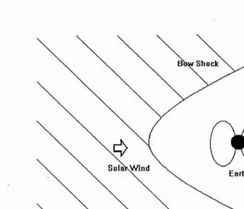
The electron density and flow velocity are roughly equal to the proton values. The pressure of the solar wind tends to compress the sunward (daytime) side of the E arth’s magnetic field and stretch out the nightside field into a long tail (see Fig 1.1). A magnetic cavity, the magnetosphere, is formed around the Earth, extending out to a distance of about 10-11 Earth radii, with the solar wind flow pressure being approximately balanced by the magnetic pressure of the E arth’s field. The solar wind is forced to flow around the boundary (the magnetopause) of the cavity. This flow is clearly supersonic with respect to the sound, Alfven and magnetosonic wave speeds, and so a stand-off shock wave forms about 2-5 Earth radii upstream of ther magnetopause, just as happens when a blunt body travels supersonically through a fluid medium. The region between the shock wave and the magnetopause is known as the magnetosheath, and consists of shocked, subsonic, heated, turbulent plasma.

solar wind parameters can vary by several orders of magnitude over a period of several months, the terrestrial bow shock is a valuable ‘laboratory’ for the study of shock physics. Multiple satellite missions, such as ISEE (International Sun- Earth Explorer) and AMPTE (Active Magnetospheric Particle Tracer Explorers), have made it possible to distinguish between time and space variations in plasma quantities, and the degree of sophistication of the instrumentation carried on board has made it possible to to make highly accurate measurements on both plasma and field quantities.

1.6 N um erical Studies o f C ollisionless Shock

waves

Although the terrestrial bow shock does provide an excellent opportunity to study collisionless shocks, it does have a number of drawbacks, not least the cost and complication of transporting measuring equipment up into space. More funda­ mentally, it is impractical to make simultaneous observations on the shock at more than a few locations. As in other branches of plasma physics, the difficulty of experiment and the intractability of the governing equations has made the nu­ merical simulation of plasma phenomena an attractive option. The first attem pt to model a shock numerically was due to Colgate and Hartm an [7] who used the charged sheet of Dawson [9] to simulate an electrostatic shock. The majority of computer codes written to study shock physics fall into three categories [34]:

Fluid codes: The multi-species fluid equations (conservation of mass, momentum, energy) are augmented by ‘phe­ nomenological’ terms describing microscopic ef­ fects, which are outwith a purely fluid description;

Particle codes: The motions of a sufficiently large number of par­ ticles are followed;

Hybrid codes: A particle description is used for the ions, and a fluid description for the electrons.

Fluid codes have the virtue of requiring the least computational effort of the methods, but the description is clearly not self-consistent in that microinstablities cannot be modelled directly, and so anomalous transport terms must be included (recall that without viscosity or resistivity, classical or otherwise, the fluid equa­ tions do not support shock solutions). Other physical effects, such as particle reflection and trapping, are also absent.

more economical in terms of computer time and storage space, but the detailed electron dynamics cannot be studied.

1.7 O utline of C ontents

In chapter two we outline the principle features of the various instabilities that have been proposed to account for the anomalous resistive dissipation in collision­ less plasma shock waves, and review their applicability. We then derive a linear dispersion relation relating the complex frequency of an electromagnetic wave to its wavenumber. We simplify this dispersion relation to the case of electrostatic waves.

Chapter three contains a derivation of the quasilinear equations, which ex­ tends the theory of chapter two to allow for the reaction of the unstable elec­ tromagnetic waves on the electron distribution function. It is shown that an asymptotic steady state must be reached in which all the waves excited evolve towards a state of marginal stability. Again, the electrostatic limit is recovered. In the next chapter we discuss in some detail the numerical methods that we chose to solve the system of quasilinear equations, and the rationale behind their choice. Although the equations were only solved for electrostatic waves, it is pos­ sible to extend the methods to electromagnetic waves: however, the complexity of the equations would mean that considerable computational resources would be required.

In chapter five we present results obtained by the numerical computer code, and discuss their applicability to the shock problem.

Shock

Earth

in te rp la i^ a ry M agnetic Field

Chapter 2

Linear stability theory

2.1 Current driven instabilities in collisionless

plasm a shock waves

There are several different instabilities that could conceivably occur in the ramp of a low Mach number perpendicular collisionless shock wave, and here we intend to review the properties of some of them. In order to be a likely contender as a mechanism for producing the “dissipation” required for a resistive shock wave, an instability must satisfy a number of criteria

[13],[34]:-1. Any threshhold value above which the instability occurs must be satisfied;

2. The growth rate must be large enough for the instability to grow to a significant level in the time it takes for the plasma to flow through the shock;

3. The instability must not saturate at too low a level;

4. The excited waves must be able to heat the plasma.

Clearly, the first stage of any study of resistive heating must be a linear stability analysis to ascertain whether or not a specific instability mechanism will satisfy

14

■

1

1

the first two criteria under realistic physical conditions. Analysis of the other two criteria is necessarily nonlinear.

Among those instabilities that could occur are [13],

[34],[41]:-1. The Buneman (Two Stream) Instability

This is the simplest of the streaming instabilities, and does not include the effects of the background magnetic field. Since it requires a relative electron- ion drift velocity greater than the electron thermal velocity, it seems unlikely to occur in a collisionless shock.

2. The Ion Acoustic Instability

Ion acoustic waves can propagate through an unmagnetised plasma at phase velocities larger than the ion thermal velocity but smaller than the electron thermal velocity. If the ions are sufficiently cold, then the wave phase velocity lies on a virtually flat region of the ion distribution function, and there is little damping. For wavelengths much larger than the electron Debye length, the dispersion relation is similar to that for an acoustic wave, hence the name. Its nonlinear heating effects were studied early on [26], [27]. For typical bow shock parameters, where usually the ion and electron temperatures are roughly the same, the cross-held currents generated in the shock ramp are not large enough to give rise to the ion acoustic instability.

3. Bernstein Wave Instabilities

the fact that they can exist for arbitrary values of the electron-ion temper­ ature ratio: however they are stabilised by the effects of either a magnetic field gradient or of orbit modifications by turbulent fields, both of which tend to ‘smear out’ the cyclotron resonances on which the instabilities are critically dependent. Very closely related is the beam cyclotron instability [30],[31], where the difference seems to be that the analysis is carried out in the electron, rather than the ion, rest frame. This class of instabilities is probably unimportant in shocks, because the instability saturates at too low a level to produce a high enough level of anomalous resistivity.

Lashmore-Davies [32] [33] has pointed out that in the presence of drifts the Bernstein waves have negative energy, so that the ions can absorb en­ ergy from the electron waves through the Landau resonance, causing the amplitude of the wave to grow.

4. The Lower Hybrid Drift Instability

Low frequency instabilities propagating perpendicularly to an inhomoge- neous magnetic field have been studied for electrostatic [28] and electro­ magnetic waves [8],[17]. The instability propagates perpendicularly with wavenumber kathe « 1) and frequency and growth rate both of the order of the lower hybrid frequency ulh = Wpi [1 4- Wpe/wce]"^^^. The ions can be taken to be unmagnetised, but the electrons are strongly magnetised. There are gradients in the magnetic field, the density and the tempera­ ture. Despite a relatively low growth rate and long wavelength, it does seem to be able to heat both ions and electrons [43]. For non-perpendicular propagation, the instability is termed the generalised lower hybrid drift instability[24]: for electrons with finite temperature, the behaviour of the instability is complex.

5. The Modified Two Stream Instability

The modified two stream [35]is similar in nature to the lower hybrid drift instability. However, the analysis of the modified two stream instability generally neglects density gradient effects but includes a component of the wavenumber vector parallel to the magnetic field. Like the lower hybrid drift instability, it is a low frequency instability (cu <C w#). The effect of a magnetic field gradient is to reduce the growth rate slightly [13]. Its proper­ ties are insensitive the the ion-electron temperature ratio and the electron plasma to cyclotron frequency ratio. Electromagnetic effects tend to sta­ bilise it for low beta and near perpendicular propagation when the relative ion-electron drift speed is greater then the Alfven wave speed. Analysis of the instability under conditions typical of a laboratory shock experiment [13], using an estimate of the expected anomalous resistivity [15] suggest that it is unlikely to produce significant electron heating. The heating rates of the modified two-stream and ion acoustic instabilities have been compared under conditions in space shocks [51] using a model based on second-order Vlasov theory. It was found that the shock widths, amounts of anomalous heating, and electric field energy predicted by the modified two stream instability were in good agreement with observations of a num­ ber of subcritical bow shock crossings, whereas the ion acoustic gave rise to much narrower shocks than observed in order to generate the larger cross­ field drifts it required for the given electron-ion tem perature ratios. For finite electron beta, the instability becomes the kinetic cross-field stream­ ing instability: this is not necessarily stabilised by electromagnetic effects for large drift velocities.

6. Parallel Drift-driven Instabilities

accelerate a portion of the electron population parallel along the electric field, producing an offset peak in the electron distribution function, which can then become unstable to parallel propagating ion and electron acoustic waves[46], possibly leading to parallel electron heating. The height of the offset peak is observed to decrease through the shock, suggesting the action of wave-particle interactions.

2.2 T he linearised V lasov equation

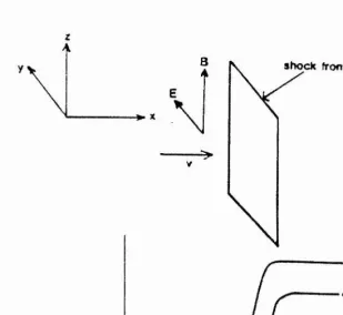
In order to determine whether a given electron equilibrium distribution is stable or unstable to small perturbations, we split all particle and field quantities into time-independent background parts and rapidly varying fluctuating parts. In all of what follows, we shall use a Cartesian co-ordinate system with the z axis aligned along the magnetic field, which is assumed to have no curvature or shear, and the x axis to be in the direction in which the background quantities vary, with the magnetic field increasing with increasing x. The y axis is chosen so that the axes form a right-handed set (see figure 2.1).

Thus:-F e(r,v,<) = /e (r ,v ) + « /e ( r ,v ,i) (2.1) H (r,<) = H o(x) + 5 H (r ,i) (2.2)

where H is any of the field quantities. It is a consequence of our assumption of slab geometry that the background fields vary with x only. The background magnetic field is taken to be:

Bo = Bo(a;)ê|| = jBq(1 -f- egæ)ê||

and the background electric field to be:

Eq = (£?a;,0,0)

i

•4

The value of Ex is not independent, but is related to the background gradients by Ampere’s

law:-f) f) p ci p ci f

— 5/e -f v . ^ 5 / e _{at dr rrie} [Eo -j- V A Bo] . - ^ 6 f e_dv = — [5E + V A 5_me B_{dv ^ ^}] (2. 6)

Equation 2.5 can be shown to be satisfied if fe is of the form;

f e — / e( ' ^ ) '^^±5 ^ ||)

where A = — {vy — ve), + (u^ — ug)^, and ve — ~ Ex/ Bq is the

‘E cross B’ drift velocity in the y-direction.

19

aj*

V A Bo = fioio = fiouo {v e + Ujv) è y (2.3) | 4 where vn = — is the drift velocity in the y-direction due to the density

gradient. This gives;

— iB - (2.4)

I^OTloe LOce

The quantity eg is of the order of the reciprocal of the length of the shock. We shall assume that the quantity tBVthe/<^ce is small, as the electrons will perform many gyro-orbits as they travel through the shock.

On assuming that the perturbed quantities are much smaller then the back­ ground quantities, and neglecting products of small quantities, the Vlasov equa­ tion

becomes:-Vx • [Eo -f V A Bo] - — 0 (2.5)

dx me dv ^ ^

and fi:

2.3 T he perturbed electron distribution func­

tion

We now solve (2.6): its left-hand side is the derivative of fe along the particle orbits in the unperturbed fields. Thus, we can integrate both sides with respect to t:

Sf. = — f [5E(r', t') + v' A 5B(r',i')] r', t') dt' (2.7)

TTlg —00 OV

The lower limit of the integral has been taken to be —oo, that is, we have ignored the effects of the initial values of the perturbed quantities. This integral will only converge for growing modes: damped waves may be dealt with by analytic continuation of the final dispersion relation. The perturbed Vlasov equation should be solved by a Laplace transform method, yielding the dispersion relation in the limit of large time, but this method is considerably more complicated mathematically. The dashed quantities satisfy the unperturbed orbit equations, viz.:

$ ( ( ' ) = - ^ [ E „ ( r ',0 + v '( i ') A B ( r ',< ') ] (2.8)

J ( i ' ) = v '(i') (2.9)

with the initial conditions that — t) = v and = ^) = r. W ith the back­ ground magnetic fields of the form used here, equation (2.8) can be solved exactly in terms of elliptic integrals. However, on our assumption of weak inhomogeneity, we only need the first-order solutions, namely:

u ^ ( t') - Vji c o s (w c e (^ ' - ^) 4 - 19)

V y { t ' ) = UJL sin(wce(t' - t) 4- Î?) 4- U£)

U||(t') = U||

x \t') — æ (t)-f — [sin(ü;ce(i^ — ^) + — sin(î9)] Wce

y'{t') = î/(t) - — [cos(a;ce(t'- t ) -}-î?) - c o s ( i ? ) ] - i - - t)

^ce z'{t') = z{t) H- U||(P - t)

Here, — v e-\-vb is the total drift velocity in the y-direction due to the ‘E cross B’ drift VE and the magnetic field gradient drift vb = ~\eBv\/Uce, All perturbed quantities are now assumed to vary harmonically, so that:

5 B (r,t) = 5Bk(a;) exp[z(k.r — Dfci)] (2.10) 5 E (r,t) = 5Êk(æ)exp[z(k.r — fltk^)] (2.11) 5 fe (r,v ,t) = 5fek:(aî>v)exp[z(k.r — Okt)] (2.12)

We only consider waves in the y-z plane, so that ^0, fcj_, k\\J. Waves thus propagate perpendicularly to both the background magnetic field and the direction in which the quantities have been taken to vary, flk = + where ojk is the frequency, and 7k the growth rate. Faraday’s law can now be used to write the perturbed magnetic field in terms of the perturbed electric field in (2.7), giving

(2-13) and the solutions to the orbit equations can be used to write the derivative of /g with respect to the primed velocity co-ordinates in terms of A, uj. and U||, all of which are constants of the motion. After changing the integration variable from

f to T — f — t, we find:

6fe = exp[~z(k.r — üy^t)]

X _TTlg / exp jz \—a± cos(ujceT -f z9) + u_L cosi? — Ü k rll Qk/ed'?(2.14)

J~oo ^

where a± = A:jLUj_/wce, Dk = Dk — k±VE — A;j|U||.The operator Q is given by:

 ,k 8 E , _{(cük - ( - 4 r + ^}

+ 5.é||

Ô A ux d v ±

^ _ r ^ D d \ d

^±,k

4

6k

È

= [±i«Ê.,kC/k + « 4 .k ê k + «S|i,k^]

- fcx«x^ + (wk -

("k - *ll“ll) i +

a

"ii&T Ux' d

(2.16)

(2.17) (2.18) (2.19)

;± dvi\

For this integral to converge, we must have 5R{0k} > 0. In order to perform the integration, we use the Bessel function generating function to obtain the identity

irvâ n ~ —oo

and thus to write the right-hand side of (2.14) in terms of known integrals. The recurrence relations for the Bessel functions may then be employed to simplify the resulting expression to the following form:

where

OO OO

G m ——oo n = —oo (2.20)

^n,k A ,k

K.k

,k

H k - k ± V D ~ ^||U || — n U ce

— [ z J ^ 5 4 k 4 + Jn 8 Éy ^ l : Vn X 4 - J n S É \ l l : W n, - k \

+ (%

-4- - ^ { n u ic e_«X 4- k±VD)-K_QU||—

d (nwgg 4- k i_ V B ) d

+ (Bk — k^V E — riLOce)-X_OUll—

dv

(2.21) (2.22)

(2.23)

(2.24)

2.4 T he perturbed ion distribution function

As they travel through the shock layer, the ions will be virtually unaffected by the magnetic field, since the ion gyroradius is much larger than the shock thickness.

Their orbits can thus be approximated by straight lines. Also, since the frequency of the waves in the shock is much larger than the ion cyclotron frequency, they will behave as if the perturbations are electrostatic. Hence, we can take the perturbed Vlasov equation for the ions to be:

The perturbed ion equation then gives:

2.5 T he dispersion relation

From Maxwell’s curl-B equation, we can derive a wave equation for the Fourier transformed perturbed electric field

k A (k A 5Ék) = - % B k - iîîk/«o E & . k (2.26)

^ a

where 5jg k is the Fourier transform of the perturbed current density due to particle species s. The sum is over all particle species. The current density is given in terms of the perturbed distribution function by

5js.k = v5/g,k dv (2.27)

/A .

J

5je,k = / [^-L COS dex + (Vi sini? + VD)éy + U||e||] e

m n

^n.k‘^rn(ax)Ên,k/e dv

/• rl

. 1

■(c'a; - ié y )v x e " ’ + - { é « + ie^jtixe"*’’ + v o ê y + U||e||

e -‘'<” - ’‘” ”-'/^)n ;'k J„(ax)F „,k X dv (2.28) Since we have:

1 P ” . I 1 m = n + p

*'«e m V./ I.

o , -- ...T-j. 1 ^ (2.29)

^ 0 otherwise

the double summation over m and n collapses to a single summation over n when the theta integration is carried out. Using the Bessel function recurrence relations once again, we finally obtain the following expression for the perturbed electron

current density: 4

5je,k = ---+ (nWgg + k±VD)Jn{a±)éy + A;jj Jn(a±)ej|] ^e^tk n

fi;,kX .(ai)Ê „,k/e dv (2.30)

The perturbed current density for each species can be related to the perturbed electric field through a conductivity tensor

<Js,k-5js,k — <^5,k ■ 5Ék (2.31)

The ion conductivity tensor is simply

e^ f V d fi

^ *m,nk / (% - k.v) ~d^

and the electron conductivity is given by:

g2 +00 f I ^

^mefik n £ o J (% - ^1% - A:||U|| - nujce) ^ (2.33)

where

Sn,k = iv s.Jn J 'Xy

-'^ t4

''°

„^W„,k

(2.34)

To obtain the dispersion relation, we simply insert (2.31) into (2.26), to give M • 5Ek = 0. In order that the electric field has non-zero value, the determinant of the tensor M must be zero, so that the dispersion relation is:

* ( k k - +X^£s,k 0

where

^ s,k — <^s,k

(2.36)

(2.36)

2.6 Sim plifications o f th e dispersion relation

The dispersion relation just derived is intractable in its present form, and must be solved by numerical methods. Even so, a number of simplifications can be made, to make numerical solution an easier and more efficient task. If, as we will do later, we only take into consideration electrostatic waves, then we can make drastic simplifications. This should be valid provided that the plasma beta is small: in this case the shock will be laminar or quasilaminar. We can obtain the electrostatic form from the electromagnetic by taking the limit c —> oo, although it is in fact much simpler to return to the perturbed electron function (2.20) and write the perturbed electric field in terms of a potential function. For waves in the y-z plane, we have

so that (2.20) becomes:

p °°

% ,k = — % E E (2.37)

OO o o

m = — o o n = — o o

where the operator J^ k is given by:

This new form of the perturbed electron function is used to calculate the current density, which is then substituted into Poisson’s equation. The dispersion relation will now have the form:

(2.38)

where Xi and Xe are the ion and electron susceptibilities respectively

Xi =

X e —

meSok

/f f r ir

Ê/

V

A ,k/e dv (2.40) „^r'oo J ü k - kxVD - fc||ü|| - nUc

The fact that the frequency Wk is much less than the electron cyclotron fre­ quency means that we can ignore all the terms in the summation in (2.40) apart from that with n = 0. For the case when the electron distribution function is an isotropic Maxwellian with a density gradient (but no tem perature gradient) and the ion distribution function is simply an isotropic Maxwellian, that is:

\ ^o(A) 1

/e(A,ux,U||) = -— - r — exp - 9 (27r)2 2;^=

(2.41)

where Vfhs = ksTsliris is the thermal velocity, the susceptibilities have the form:

1

Xz = [1 + (&)] (2.42)

26

X e —

(o =

4 + 2— — xJo(«x)Z(^o)exp(-x^)rf;

k^^hc

Ok k±_VE

X

(2.43)

\/2^||2^f Ae

where \ds is the Debye length for particles of species s, vn = — cjyu^g/wgg is the

drift velocity induced by the density gradient. Z is the plasma dispersion function [12], defined by

exp {—x'^)

x - i

dx

Because vb depends upon ux, will depend upon x, and so the integral in

(2.43) must be evaluated numerically. If we ignore the effects of the magnetic field gradient (which should be less im portant than those of the electric field for low beta plasmas) but retain the electric field, the integral may be evaluated analytically using the relation:

to give:

X e =

De 1

+

(Ok

— kj_VE — k_LVN)

y/^k^^Vfhe exp (—A^)/o(A^)Z(fo)

(2.45)

(2.46)

where A = k_iVthel<^ce- When vn = 0,this is the same as the dispersion relation

for the modified two stream instability (for example equation (4) of [35]).

Finally, in cases where the ions are cold, that is to say, (2^ k • v, by expanding the denominator of (2.42) and retaining only the lowest order term, we obtain:

Xi =

2.7 N um erical solutions o f the dispersion rela­

tion

Since the literature on the linear stability analysis of cross field current- driven instabilities is substantial, we do not propose to devote a large amount of space to the solutions of the linear dispersion relations derived. However, it is interesting to consider an anisotropic distribution function, that is with Tgi ^ Te|j, where

Tel. and Te|| are the electron temperatures perpendicular and parallel to the back­ ground magnetic field, and to study the dependence of the growth rate of the in­ stability on the tem perature anisotropy = Tex/Te|[. If we define Ug|I = ksTew/rne

and UgjL = keTe^/me, then an appropriate background distribution function is

= (2x)3/^ u î X l (2.48)

from which we can derive the following relation for the electron susceptibility:

w ,

X e — pe _{X i :} xJq{s x) (w — k_LVE)

V2k\

+

e|| \ k ± 6 B U e ± ‘^ X ^

y/2k\\u_dl

(2.49)

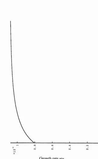
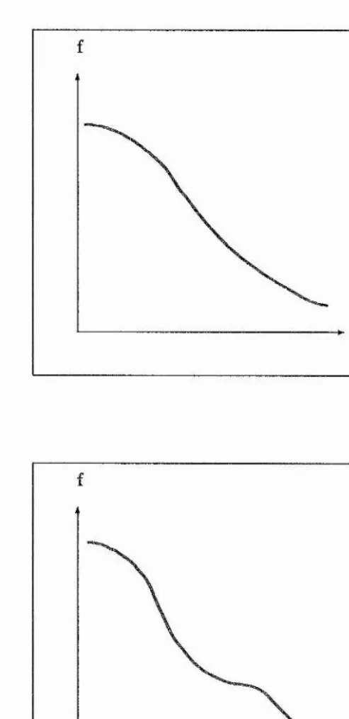
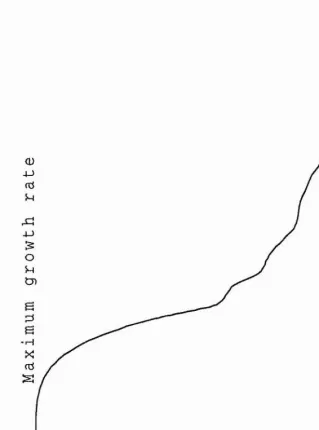
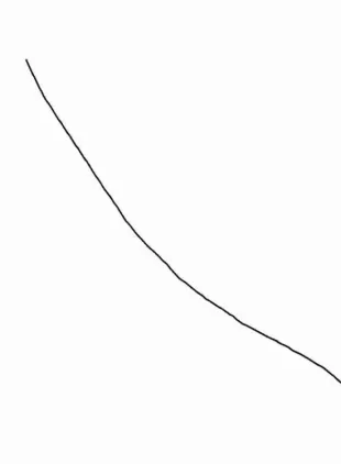
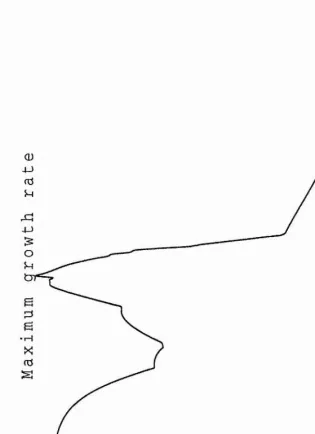
Figures 2.2 and 2.3 show plots of the real frequency and growth rate (mea­ sured in units of the electron cyclotron frequency) respectively for the mode with k±Ue±fcOce = 1.0 and k^^Uei./u>ce = 0.1 as Tgx is held fixed and Tj| increased, as would happen during a period of parallel electron heating.

28

shock front

y

X

Figure 2.2: Frequency versus temperature ratio

î

I

-f-s

:'î ‘I

Real frequency: co/co,_ce

Figure 2.3: Growth rate versus temperature ratio

I

I

Chapter 3

Derivation of the Quasilinear

Equations

3.1 Q uasilinear theory

In the last chapter, we linearised the Vlasov equation about an unstable equilib­ rium, and subsequently solved for the perturbed electron distribution function. On using Maxwell’s equations this yielded a linear dispersion relation, so that given the value of the wave vector k, we could calculate the value of the complex frequency H- i')k- We now want to be able to determine the change in the background electron distribution function caused by the growth of the waves in the system over a time-scale larger than that for which linear theory is valid. To achieve this, we employ quasilinear theory. This is the simplest non-linear theory of plasma instabilities, and was first developed for unmagnetised plasmas by Drummond and Pines [10] and Vedenov, Velikov and Sagdeev [49], and later generalised to electromagnetic instabilities in a homogeneous magnetic field by Kennel and Engelmann [25], and also to the case of electrostatic waves propagat­ ing through an inhomogeneous plasma [4].

The principles of quasilinear theory are as follows: the Vlasov equation is, as

before, divided into a background part, which describes the action of the waves

on the slowly varying unperturbed distribution function, and a fluctuating part | ■1 to describe the rapidly varying behaviour of the system due to the influence of the

waves. To solve the latter equation we decompose the perturbed quantities into a set of Fourier modes, and ignore interactions between the different wave modes, so that the perturbed distribution function satisfies a linear equation, which can then be solved. The perturbed distribution function is then substituted into the unperturbed equation, yielding a diffusion-type equation. In general, particles will diffuse in velocity space in such a way so as to push the system into a stable (or marginally stable) state. Not surprisingly, diffusion is strongest for

those particles with velocities close to the phase velocities of the waves (‘resonant | diffusion’), and weaker for the remaining particles.

3.2 The electron quasilinear diffusion equation

We now derive an equation to follow the evolution of the electron distribution function. The derivation substantially follows that of [25]: however, we have allowed the background magnetic field to vary slowly in the x-direction. We start by averaging the Vlasov equation in order to remove all rapidly varying terms. However, we allow the background distribution function to vary (slowly) in time and retain the second order term involving the wave field and the perturbed distribution function. This was neglected in the linear theory, but is retained here as it describes the action of the wave spectrum on the background distribution. The averaged Vlasov equation is:

removes all terms linear in the perturbed quantities. Since the situation under consideration is time-dependent with waves in the y-z plane, we could take:

where Ly and measure the periodicity length of the system in the y and z directions respectively.

We now need to derive an expression for the perturbed distribution function. To do this we Fourier analyse the perturbed quantities in time and space:

8B{r^t) = ^ 5Bk(a;) exp[z(k.r — Ok^)] (3.3)

k

6E{r^t) = 8Éy^(x) exp[z'(k.r — Hk^)] (3.4)

k

^ /e (r,v ,t) = 5Z<Ç/ek(æ,v)exp[z(k.r ~ HkO] (3.5) k

We have assumed that the system is periodic in the y and z directions, so that the wave number vector is forced to take on a number of discrete values. This is purely for algebraic convenience, and later we will let the periodicity lengths

Ly and become infinite, in which case the wave number spectrum becomes continuous, and the sums in our expressions become integrals.

The time-independent distribution function used in the linear stability the­ ory of the previous chapter was necessarily independent of the gyroangle theta (defined by tant? = ■). Since the fundamental idea of quasilinear theory is that the background distribution changes slowly compared to the perturbed distribution function, then its variation with the gyroangle should also be weak. If we then expand the background distribution function in terms of the reciprocal of the electron cyclotron frequency [25] :

/e(A, VI, Ï?, V||, t) = /M(A, Vj., Î?, V||, t) 4- -i-/W (A , Vj., V||, t) -f 0 ( - ^ ) (3.6)

UJr.

Using 3.1, and remembering that the rate of change of fe due to the waves is small, we see that:

g/i°» n

This valid as long as the growth rates of the waves are all much smaller than the cyclotron frequency. For the instabilities considered in this thesis, we have:

and

<

so that we are clearly justified in making this assumption. The higher order terms in (3.6) can be removed by integrating (3.1) over the gyroangle (gyroaverging) and noting that the terms /]”! are all periodic in theta. We are left with an evolution equation for . We will drop the superscript so as not to overburden the notation.

Since all the perturbed quantities are real, a number of symmetry relations has to be obeyed:

= (3.7)

«É_k = (3.8)

s h - k = (3.9)

n_k ~ “ ^k (3.10)

^

dv

(3.11)

The right-hand side is necessarily real, on account of the symmetry relations (3.7) to (3.10).

From chapter 2, the perturbed electron distribution function can be written as:

«/e,k =

E E

m n

where

Gm.k = i — e-(™-’‘)’'/V „ (a x )fi;‘k#„,k/, _Tn>e (3.13) We now substitute this into the right-hand side of (3.11), use (2.13) to eliminate 6Bk, and change velocity co-ordinates to cylindrical polars. The gyro-averaged background Vlasov equation is then:

1 /•27T .

m. (3.14)

with

Ac — ^0 + Â4. -f- %Cj^ A_ -I- iC

-dê (3.15)

— [ ( % - kj_VD - kjLVB - A)||V||) % , k T i (Uk - A:||V||) 6B^,k

A:j_V||4$A|,kj (3.16)

The operators Aq and A± were defined in chapter 2. The form of Cq is not impor­

tant; we shall see later that when the 0 integration is carried out it disappears. To calculate the right-hand side of 3.14, we need to evaluate the term:

/•2ît ^

1 /'27T

2 Ï (3.17)

36

If we substitute for Ac from 3.15 and for 5/e,k from 3.12, then:

d _id

+ e' A_ + %C_ ^fe,kd'à

(3.18)

The À operators and C± are all independent of theta, so that we can integrate the terms proportional to by parts, that is:

and

thus: 1 /■2’r

Jo

27t Jo d 'à (3.19)

'^lo

= E E ^ {«’■'’"-’•'"io +

(Â+ + C+)

+ ( i _ + C_)}* G„„kdiJ (3,20)

We can now use (2.29) to perform the theta integration. As before, the double summation reduces to a single summation over n. Thus:

r p m ^ d ,= E { [ a r + f ô ] * + ( 3 - 2 1 )

1 fZvr

2?r

where

'

A i l = (3.22) 1

f i l = ( ^ + ^ n - l , n , k + ^ - ^ n + l , n , k ) (3.23) _f4

On substituting in ^/e,k from 3.12, it is possible to perform the theta-integration, reducing the double sum to a single sum.

We now expand the right-hand sides of equations (3.22) to (3.24) in turn:

K k ] * = [ - ^ { i S É ^. A + S É y , A +

— [2 + SÉyf^Gk + [~-ln+lll3,kA .,k/e

= ^ { - % , k % ( 2 - ' ^ % , k ê k (

- ii:x«£||,k^k (^1 11+ ^1= 1.) y X n;]^F„,k/e

Ai+1 H" d n ~ l

SÈ,,kÛkJ'n + « 4 . k G k | ^ ^ +

x % lf .,k A (3.25)

A similar process gives;

[A5c] = ^ [(% - kx_v^ % ,k - i (^k - <

5

X [ ~ ‘^^-l^n,îcAi,k/e

nwr

2vj_ [ - i (fik - kj,VB) 6 & ,k /; - ^ ( % - fcxoli) SÉy,k ~ ^ 3 ,k A .,k /e (3.26)

and finally:

[^Ük]* =

I

4- k±v^\ d

dk vx. dvx. 4- (% - kx_VD)

av||_

d

j/,k

dv\ ll,k

(3.27)

We now substitute (3.25), (3.26) and (3.27) into (3.21), to get:

+ ^ + ^ n - l , n , k + ^ t < J n + l , n , k + C *+ (^7i - l ,7i,k + Ct G n X - l ^ n ^ k

38

■Î

+

(Ok — k^vs)

v± JL

kL \ %;±

(% - * i« ||) - VB

^ 1 I (» k -fcx O ||)'

1 ^ \ , r d V ± d v ± )

Jn

d / A 1 v u

Jn

(3.28)

We now use the operator identities;

G k - = - G k -_{v± v i}

H k J -_Vx = ^ A k - %

V±

in (3.28) to write (3.21) as:

è /o

■k

JL

E j ' ^ & k % +

n L

+ ^By,k%i,k^ + <^Al.k^n,k*^}

The evolution equation for the electron distribution function is thus:

(3.29)

%

dt

(Ok — k±vsj

Okvx +B ;,k

(3.30)

This equation can be written in the form of a quasilinear diffusion equation

d f dt

Dp =

d y . D .. dfi

^ E E ®AkB„,ka„,k

(3.31)

an,k = «n,A,kêA + «n.lkêx + ^^n,||,kê||

^ n,A ,k — \fk± ,V x.J^ S È x^

\i-\-(Ok - A)j|V||) Jn8Èy;^ H- fcxV|| Jn^B||.k] (3.33)

^n,±,k ~ (^k “ kx.VE ~ ^ll'^ll) Jn^^x,kA

(" k - *||"||)

(n . ^ + k,v s ) j^^É ,,k

Il t)x (3.34)

«n,||,kê|t - ^ [zA:(|VxJi^Ba,,k+

(nwce 4- k±V]x)

(Ok ^X^Z) V>üJce) ^n^B|| kj (3.35)

Il = AêA 4- vxêx 4- t;||é|| (3.36)

If there are no spatial gradients in the background quantities then the above equations are equivalent to equations (2.26) and (2.27) of [25]. It can be shown (see Appendix ) that equation (3.31) conserves energy.

3.3 T he Q uasi-H T heorem

We can apply the arguments of Kennel and Engelmann [25] to (3.31) to show that the system must tend to some marginally stable state as t tends to infinity. We accomplish this by defining the functional

He = ^ / fedfi (3.37)

Differentiating this with respect to time, using (3.31) and integrating by parts gives us:

dHe

dt

-

< 0

dll

( 3 .3 8 )

Since He is clearly positive definite, and is negative semi-definite, H must decrease monotonically in time until it reaches a steady state with = 0. This must occur either when 'Yk = 0 or, since He is a sum of positive definite terms,

df. _{( 3 .3 9 )}

In the latter case we arrive at a contradiction, as the perturbed distribution would have to be identically zero, in which case no waves would be excited. Thus, in the limit of infinite time the electron distribution function must tend to form such that all the waves excited are stable.

3.4 E volution of field am plitudes

On the long times cale, the electric fields will change in time according to:

^«,k(4% k(^) = -^a,k(0)-E^,k(0) exp 2'jy,{t')dt' (3.40)

This expression can be written as a differential equation, giving:

3.5 Q uasilinear diffusion equation for electro­

static waves

In the same way that we simplified the dispersion equation by assuming that the electric field was derivable from a potential, we can write the diffusion tensor as:

where

bn,k = -ki.eA + (3.43)

h{ t) = |% (^ )|^ (3.44)

7k is the intensity of the wave with wavelength k. This quantity will evolve in time according to:

^ = 2% /k (3.45)

(3.; as was done in the dispersion relation.

It is possible to simplify both (3.32) and (3.42) by ignoring the n ^ 0 terms, i|

3.6 Q uasilinear diffusion o f th e ions

If we make the assumption of negligible ion tem perature again, we can derive equations to describe the evolution of the bulk ion parameters under the action of the turbulence. Because of the large mass of the ions, we can neglect the effect of the magnetic field on them. The quasilinear diffusion equation for the ions under the last assumption is:

(3.46)

where;

To derive an equation for the rate of change of the ion therm al velocity, we multiply (3.46) my ~miV^ and integrate over velocity;

^

= (3.48)

If the ions are cold enough, i.e. kvthi < then we can expand the denominator in the above:

(Ok - k • v)

1

1

Hk

+

k • V

Ok + • •

and so j d f l

d t J -m iv^fidv = %

. c

I — m.

k • V

Ok fik fik

k •

I

fidv

1

% 4"...

(3.49) k (‘.'k + 7k)

Chapter 4

Solution of the Quasilinear

Equations

4.1 T he quasilinear equations

The system of equations for the evolution of the electron distribution function under the action of electrostatic turbulence is:

(4.1)

d f , d '

dt d f i (4.2)

hr.d\c\ k^VD - «||U||

De = (4.3)

bo — — H êx + ^||ê|| ux

27k/k (4.4)

dt

fl = Aca + uxêx + u||ê(i (4.5)

Only the electron distribution function has been allowed to evolve in time: the ions are taken to have a constant temperature T{ <C Tg.

In order to follow the evolution of the system, the folowing scheme is used to advance the ysytem through a small time interval:

1. Given the distribution function /g, the dispersion relation is solved for a range of values of k± and A:|| to give the complex frequency

2. The diffusion tensor De is calculated;

3. The electron distribution function is advanced to the next time level;

4. Finally, the wave intensity function is advanced.

This process is repeated until either a prespecified time value is reached or all waves in the system have stabilised.

4.2 Solution o f th e dispersion relation

The numerical solution of the dispersion equation poses not inconsiderable prob­ lems. Normally, one is able to represent the distribution function by a known, analytical function: usually one chooses a Maxwellian distribution with appro­ priately chosen tem perature and density, as was done above. This has the great advantage that the singular uy integral can be written in terms of a tabulated function, the plasma dispersion function.

In the situation under consideration here, however, the electron distribution will evolve in time, and even if it were initially Maxwellian, it would soon cease to be so. This change in form is crucial to the theory, since the growth rate is de­ pendent on the shape of the distribution, and we are hoping that the distribution function will change so that the instability will cease.

where L is the Landau contour, that is, from minus infinity to infinity under­ neath any singularities of the integrand. To evaluate such an integral numeri­ cally (as does the Ferguson subroutine for the evaluation of the plasma dispersion function), one would have to be able to evaluate g { u ) off the real axis. For a

Maxwellian plasma, g { u ) = exp(—u^), and this process poses no problems, but

we intend to solve the diffusion equation using a finite difference method, which means that /g(æ, ux, U||,t) may only be calculated for real uy .

In order to obtain an approximation to and 7k, we considered the use of two different strategies, a small growth rate approximation method (method 1) and an orthogonal polynomial expansion method (method 2).

4.2.1 M eth od 1

Split K into its real and imaginary parts K = + iK{, then, assuming that

Ki <C Kr

7k < Wk (4.7)

we can Taylor-expand K about Wk, and get, on dropping small terms:

7fr(wk) = 0 (4.8)

7k = - K i dKr (4.9)

In other words, we find the solution of the real part of the dispersion relation for real Hk, and then calculate the growth rate from the imaginary part of the dispersion relation and the gradient of the real part, both of which are to be evaluated at Wk. The problem of evaluating fe off the real axis is now solved, since Kr now involves the Cauchy principal part of the uy integral, which can be evaluated by putting fe to be a Maxwellian with density and tem perature equal to those of the true distribution function. In K{ the smallness of 7k means that

we can replace the resonant denominator by the Dirac delta function:

Kr = 1+ x M + X ^ '

fd __ I

Wk

K i = / / J o { a i ) <^{wk - kj^VD - fc(|U|j) bo • ^ uxduidx;j|

JO J ~oo O il

(4.11)

where s = \/2ks,Vthel^ce^ m = —tNV^f^Jujce, m = {l/no)dno/dx

(wk - k±VD) y/2k\]"^the

(4.12)

and

oo

= - 2e -(' f \ ‘"dz Jo

(4.13)

The function here denoted Zr{^) is related to Dawson’s integral [1]

4.2,2 M eth od 2

We shall go back to the dispersion relation (2.38),(2.40) and (2.40), but we have not specified any particular distribution function. We now expand the distribu­ tion function in terms of a set of known functions, namely the Hermite polyno­ mials [1].

/e(A,UX,U||,t)

(27t)2 the

(4.14)

It turns out that a similar expansion in the perpendicular velocity component is not necessary. Such polynomial expansions have been used in analytical and numerical studies of the non-linear Vlasov equation [22],[2],[3]. However, to our knowledge, they have not been used to solve the linear dispersion relation for an arbitrary distribution function, as here. The Hermite polynomials are defined by the generating function:

exp(— -f-2su) = ^ Hm(v) m\

(4.15)

We now substitute the expansion 4.14 into the dispersion relation. The elec­ tron susceptibility %e is then:

1 noe^ ^ r /■“ J2(ax) Xe

_rrie

_Cok'

_^

_{Jo u>n - k^\v\\}

d {ncüce + kjiVB) d d

-k i.—

1 w,pe

dK

W /

dv\ dv\\ /e(^'l,^||,^) uxduxdujj

noo roo

—oo Jo _^IFII

- k dfm

aA

(nWce + ks,VB) d f

V± + A:,,/,m I % ^112