Clare B. Embling
A Thesis Submitted for the Degree of PhD at the
University of St. Andrews
2007
Full metadata for this item is available in the St Andrews Digital Research Repository
at:
https://research-repository.st-andrews.ac.uk/
Please use this identifier to cite or link to this item:
http://hdl.handle.net/10023/640
This item is protected by original copyright
distributions off the west coast of
Scotland
Clare Beth Embling
A thesis submitted to the University of St Andrews for the degree of
Doctor of Philosophy
School of Biology
Sea Mammal Research Unit
I, Clare Beth Embling, herby certify that this thesis, which is approximately …..…….. words in length, has been written by me, that it is the record of work carried out by me and that it has not been submitted to any previous application for a higher degree.
Date:………...
Signature of Candidate:………
I was admitted as a research student in October 2003 and as a candidate for the degree of PhD in the School of Biology in October 2004; the higher study for which this is a record was carried out in the University of St Andrews between 2003 and 2007.
Date:………..
Signature of Candidate:……….
I hereby certify that the candidate has fulfilled the conditions of the Resolution and Regulations appropriate for the degree of Doctor of Philosophy in the University of St Andrews and that the candidate is qualified to submit this thesis in application for that degree.
Date:………..
Signature of Supervisor:………
In submitting this thesis to the University of St Andrews I understand that I am giving permission for it to be made available for use in accordance with the regulation of the University Library for the time being in force, subject to any copyright vested in the work not being affected thereby. I also understand that the title and abstract will be published, and that a copy of the work may be made and supplied in any bona fide library or
research worker.
Date:………
Abstract i
Acknowledgements ii
Chapter 1 Introduction: Setting the scene 1
1.1 Predictive models in ecology 1
1.2 Aspects of predictive environmental modelling 3
1.2.1 Direct or indirect predictor variables? 3
1.2.2 Spatial scale in ecology 4
1.2.3 Autocorrelation in predictive modelling 6
1.2.4 Model evaluation: cross-validation 8
1.3 Cetacean species off the west coast of Scotland 9
1.3.1 Harbour porpoise (Phocoena phocoena) 9
1.3.2 Delphinid species 11
1.3.3 Sperm whales (Physeter macrocephalus) 15
1.4 Oceanography of the west coast of Scotland 18
1.4.1 Shelf waters 18
1.4.2 Rockall Trough 19
1.4.3 Faroe-Shetland Channel 20
1.4.4 Offshore biological oceanography 21
1.5 Monitoring species distributions using passive acoustics 21
1.5.1 Passive acoustics for harbour porpoises 22
1.5.2 Passive acoustics for sperm whales 23
1.5.3 Passive acoustics for delphinids 24
1.5.4 Passive acoustics in this study 25
1.6 Cetaceans and noise 26
1.7 Thesis structure 28
Chapter 2 Predictive models of delphinid distributions off the west coast of Scotland: Evaluation of autocorrelation & temporal scale 48
Abstract 48
2.1 Introduction 49
2.2 Methods 52
2.2.1 Data collection 52
2.2.2 Environmental data 55
2.2.3 Acoustic data analysis 57
2.2.4 Statistical analysis 60
2.3 Results 66
2.3.1 Environmental variables 66
2.3.2 Effect of ‘acoustic autocorrelation’ on model selection 72
2.3.3 Effect of year on model selection 75
2.3.4 Effect of change in spatial extent on model selection 77
2.3.5 Effect of month on model selection 78
2.4 Discussion 82
2.4.1 Passive acoustics & problems of autocorrelation 82
2.4.2 Model robustness in time and space 83
2.4.3 Habitat preferences of delphinids off the west of Scotland 87
2.4.4 Conclusions and further work 90
2.5 References 92
Chapter 3 Predictive models of sperm whale Physeter macrocephalus distributions off the west coast of Scotland: Evaluation of
spatial scale 97
Abstract 97
3.1 Introduction 98
3.2 Methods 100
3.2.1 Data collection 100
3.2.2 Environmental data 100
3.2.3 Acoustic data analysis 101
3.2.4 Statistical analysis 104
3.3 Results 108
3.3.1 Environmental variables 108
3.3.3 Model selection: spatial robustness between areas 114
3.3.4 Model selection: spatial robustness with scale 120
3.4 Discussion 121
3.4.1 Influences of autocorrelation & scale on robustness 121
3.4.2 Habitat preferences of sperm whales off west Scotland 124
3.4.3 Conclusions 128
3.4.4 Further work 128
3.5 References 129
Chapter 4 Predictive models of harbour porpoise Phocoena phocoena distribution in the Inner Hebrides, Scotland: Evaluating the
effect of survey technique, time & space on model robustness 135
Abstract 135
4.1 Introduction 136
4.2 Methods 139
4.2.1 Data collection 139
4.2.2 Environmental data 141
4.2.3 Acoustic data analysis 144
4.2.4 Statistical analysis 146
4.3 Results 151
4.3.1 Environmental variables 151
4.3.2 Model selection: visual vs acoustic 158
4.3.3 Model selection: temporal robustness with year 167
4.3.4 Model selection: effect of expanding survey extent 172
4.4 Discussion 175
4.4.1 Comparing visual & acoustic predictive models 175
4.4.2 Model robustness over time 177
4.4.3 Model robustness over space 178
4.4.4 Harbour porpoise habitat preferences 180
4.4.5 Conclusions 184
Chapter 5 The relationship between delphinid and herring Clupea
harengus distributions: evaluation of a direct predictor
variable 192
Abstract 192
5.1 Introduction 193
5.2 Methods 197
5.2.1 Data collection 197
5.2.2 Analysis 199
5.3 Results 205
5.3.1 Survey data 205
5.3.2 Correlation between delphinid and herring distributions 207
5.4 Discussion 215
5.4.1 Correlation between delphinids and herring 215
5.4.2 Conclusions 220
5.5 References 222
Chapter 6 General discussion 228
6.1 Synthesis 228
6.2 Distribution and habitat use 229
6.3 Evaluation of predictive models 234
6.3.1 Temporal scale 234
6.3.2 Spatial scale 235
6.3.3 Direct versus indirect predictors 237
6.4 Survey effects on predictive models 240
6.4.1 Autocorrelation 240
6.4.2 Survey methodology 241
6.5 Future applications 242
6.5.1 Recommendations 245
6.6 References 248
Appendix Additional results for all chapters A1
A.1 Chapter 2 – delphinid model tables & figures A1
A.2 Chapter 3 – sperm whale model tables A5
A.3 Chapter 4 – harbour porpoise model tables A6
i
The main purpose of this study was to produce and test the reliability of predictive
models of cetacean distributions off the west coast of Scotland. Passive acoustic and
visual surveys were carried out from platforms of opportunity between 2003 and 2005.
Acoustic identifications were made primarily of harbour porpoises (Phocoena phocoena),
delphinids, and sperm whales (Physeter macrocephalus). Generalised Additive Models
(GAMs) were used to relate species’ distributions to a range of environmental variables
over a range of temporal and spatial scales.
Predictive models of delphinid distributions showed both inter-annual and inter-month
variations. Combining data for all months and years resulted in a model that combined
the environmental influences from each monthly and yearly model. Overall, delphinids
were found to associate with the deep (> 400 m) warm water (10.5°C-12.5°C), and in
areas of deep thermocline.
Relationships between sperm whales and environmental variables were consistent over
changes in grain size (9 km or 18 km), but not between areas. Although sperm whales
were distributed in deep water characterised by weak thermoclines and strong haloclines
in the most northerly area (Faroe-Shetland Channel), they were found in deep productive
areas with cold surface temperature in the more southerly waters (Rockall Trough).
Within the southern Inner Hebrides, high use areas for harbour porpoises were
consistently predicted over time (in years) and with differing survey techniques (acoustic
versus visual), but not over space (southern Inner Hebrides versus whole of the Inner
Hebrides). Harbour porpoises were mainly distributed in areas with low tidal currents
and with higher detection rates during spring tides.
The use of prey as a predictor variable within models of delphinid distribution shows
some promise: there were correlations between delphinid and herring (Clupea harengus)
in shelf-waters in 2005 but not in 2004. These models can be used in mitigating acoustic
ii
Acknowledgements
The PhD is a journey of self discovery, a roller-coaster ride that lasted 4 years for me. I’ve spent the PhD either laughing or crying, but it’s an adventure I wouldn’t have swapped for the world. To spend 4 years studying something that fascinates you is like
living a dream, and makes the roller-coaster ride well worth the trip. I’d love to share the many ups and downs… the frustration of trying to solder a hydrophone plug with a gas soldering iron on the back deck of a boat in blowing wind and rain… the joys of seeing a humpback rise out of the water mouth first, fishy breath pervading, kittiwakes fleeing the sea surface and sprat spilling out of the huge mouth. But this would be a thesis in itself. The adventure that was this PhD would not have been possible without the support of a
whole host of people, who I’d like to take the opportunity to thank…
Firstly, I’d like to thank my supervisors: Dr Jonathan Gordon and Professor Philip Hammond. Jonathan taught me everything I know about hydrophones: how to build one, how to gut one and how to blow one up (sorry Jonathan!!!). He was always at the end of
a phone whenever I was having equipment problems and ready to send spares with lightening rapidity to the nearest port. And I always felt welcome in his home – so thanks must also go to Kate, Alex & Emma for letting me pop around & eat your food whenever I was on the prowl of equipment or help. Phil has been my little haven of calm in amongst the madness of fieldwork, so thank you for all the supporting words when I needed them. And thank you to both of you for all the support and feedback you’ve
given me during the write-up phase, and all the interesting discussions about my analysis and results.
Huge thanks to my funders: NERC and DSTL, especially to Graham Jackson, Claire Burt, Matthew Summers, Ed Harland (Qinetiq) and Ben Maughan (UKHO) for
organising my visit to pick their minds in the middle of my PhD.
All my fieldwork was carried out from platforms of opportunity, so this PhD would not be here today if it weren’t for the generosity of the Fisheries Research Services (FRS), the Scottish Association for Marine Science (SAMs), the National Oceanographic Centre (NOC) and the Hebridean Whale and Dolphin Trust (HWDT). I’d like to thank each
iii
Firstly, the Faroe-Shetland Channel hydrographic surveys carried out by FRS allowed both Sónia Mendes and I to hitch aboard and tow our hydrophone – mainly thanks to Bill Turrell and George Slesser. At which point I also have to give a massive thank you and hug to Sónia Mendes for being the best co-worker I could have asked for, and for smiling
despite the difficulty of overlapping interest in the sperm whale data. You’ve become a great friend, and I hope I get to hike the mountains and sail the seas with you in our Zissou red woolly hats for many years to come. The rest of the team on FRV Scotia were true stars: Malcolm & Dougal especially for keeping us both laughing all the time, but also all the scientists, cooks and crew of the FRV Scotia. I would just like to make a special mention of Richard ‘Dick’ Shelton, who taught me about the Atlantic adventures
of salmon, entertained me in his book ‘The Longshoreman’ and has often popped in complete with hunting rifle to check up on me in St Andrews… thanks Dick!
The participation on the July 2003 and October 2005 Ellet Line surveys were thanks to the generosity of Toby Sherwin (SAMS) and John Allen (NOC). Sónia and I had a trip
of a lifetime aboard the rusty but much loved RSS Charles Darwin travelling through Force 12 storms to Iceland and back. I don’t think I can ever thank the other scientists and crew enough for making the trip so special and for making us feel so welcome. Special thanks have to go to Maria Nielsdóttir for giving us the worked up chlorophyll data (sorry for not using it!), to Peter Lamond for teaching us about acorn worms and other critters from the depths, for all the technicians, cooks for keeping us fat, and a great
crew. The trip can be enjoyed for many years to come as ‘CD176 – the movie’.
The generosity of Paul Fernandes & Dave Reid (FRS) allowed me to hitch aboard the herring abundance surveys on the west coast of Scotland for the first time, and trusted me enough to allow me to tow a hydrophone between fish trawls – thank you! These surveys
would have been a real struggle without Eric Armstrong, who provided huge support especially on my first ever survey with a novel but very noisy and leaky hydrophone. I spent many hours of fishy fun with the other scientists: Emma Hatfield was a great cabin buddy, and she & Finlay Burns taught me all I know about fish id, determining the maturity state and sex of a herring, and many more weird and wonderful fishy facts.
Thanks also to Isobel Rombouts for joining me on one of my surveys so that I didn’t have to try and stay awake during all the 20 hours of each survey day! Thanks to each and every one of the science and boat crew of the Enterprise – I’ve never met such a great bunch of fishermen! An additional thank you goes to both Eric and Paul for processing the herring survey data for the west coast, and for all the discussions that formed my
iv
a survey buddy who made me laugh; (b) joining in my brain storming session about my dolphin-herring analysis; (c) suggesting the Multinomial Logit Model to me; and (d) for letting me adapt his code.
How can I ever thank the Hebridean Whale and Dolphin Trust for letting me join the
team, help on the trips, and for letting me use their data? The trips on the Silurian were pure indulgence: sailing around the stunning islands of the Inner Hebrides, mooring at a different port on a different island every night, and exploring the remotest parts of the west coast of Scotland. My love of the west coast is a result of these trips, and I came to think of Tobermory as my second home. So firstly massive thanks to Juliet Shrimpton,
who ran all the surveys, kept the hydrophone working, and kept all the volunteers happy and on their toes for spotting critters during all 3 years of surveys. I miss our trips
together, and I hope we’ll get to do trips together again in the future. Thanks also have to go to each of the skippers who’ve managed to combine the odd requirements of
surveying an area evenly to the whims of scientists and the weather and the location of
ports, tides etc., and especially to Duncan Cameron who’s kept the boat in tip-top condition (but stop with the anti-bac!). First mates Jamie Spears and Marcus Walters were great at juggling between keeping the boat sailing and helping out with the science… quite some task – so thank you! In 2005, Marjolaine Caillat was a massive support while on the boat during her masters, and helped me to stay laughing despite massive computer failure on the trip where we tried to run two hydrophones from one
computer (don’t try it!). Marjolaine & I with huge phone support from Guillaume managed to rebuild the computer and only lost out on a day’s survey effort. Talking of equipment failures on the Silurian, I also have to thank Roy Wyatt (Seiche Electronics) for such good support for the porpoise boxes. Finally, back at base thanks go to Cally
Fleming, Barbara Weir, and Fiona Quarmby who provided lots of support and smiles. But of course none of these surveys would have been possible at all if it weren’t for the hard work from all of the HWDT and Earthwatch volunteers – I had so much fun working with you all, the trips would never have been so much fun if it weren’t for your enthusiasm.
This project was also carried out in conjunction with Phil Gillibrand (SAMS), Steve Gontarek (SAMS) and Geert Arts (SMRU). Phil has been a great support in processing my environmental data for me, and being a great guide through the complexities of physical oceanography. Steve designed the fabulous tool for ArcGIS9 that loads all manner of weird and wonderful environmental data into a GIS database, and allows you
v
it. Thanks Steve for the great tool, and for being at the end of an email or phone
whenever I needed help. Geert deserves huge thanks because I benefited from travelling in his wake – he did much of the work sourcing the environmental data, so that much of it was ready already when I needed to start my analysis. I have to tag on extra thanks to
Clint Bight at this point for all the unpaid computer support he provides to the
department, and for all the GIS problems he’s helped me with despite being overrun with his own work.
Lots of SMRU & CREEM folks have given me a lot of help too: Rory Beaton, Colin Hunter, and Julian Dale gave me huge amounts of support in the early hydrophone
building days. And of course thanks to Simon Moss for letting me take over the boat shed with my hydrophones and teaching me how to use a drill. Ana Katerina Alves and Anneli Englund were great helpers with the tedious task of processing some of my massive pile of acoustic data – thanks for doing a great job AND staying sane! Extra fieldwork assistance was provided by Tess Gridley, Cormac Booth, Caroline Weir and
René Swift when either Sónia or I couldn’t make the survey – thank you for doing a fantastic job! And Tess you were a great boat-buddy! Thanks for the sounding boards for ideas: Mike Lonergan, Doug Gillespie, Sinead Murphy, Simon Northridge, Charles Paxton, Monique Mackenzie, Vincent Janik and the bioacoustics group.
Thanks to all my proof readers! They are: Eric Armstrong, Peter Stevick, Phil Gillibrand, Paul Thompson, Kate Brookes, Simon Elwen and of course my long-suffering
supervisors. Please don’t blame them for my writing style – as Mrs Kubiak once wrote on my English homework ‘too waffly’… I hope I’ve improved since then Mrs Kubiak!
Finally, huge thanks have to go to my ‘keep Clare sane’ team. Firstly, Gill Perris (née
McLaughlin) thanks for inspiring me in February 2000 to change fields from engineering to biology – this thesis would never have been here if it hadn’t been for your inspiration. Thank you too to my coffee buddy and old flat mate and token non-scientist pal Amanda Beattie – you’ve kept me smiling all through my PhD. Thanks too to my long-suffering office buddies and great friends: Sonja Heinrich, Louise Cunningham, Simon & Lisa
vi
Ross Culloch; Barbara Cheney; Tim, Carrie, Sam & Megan (& Sorrel) Barton; Line Cordes; Theoni Photopolous; Gillian Riddoch; Paul, Helen & Emma Griffiths (& the gang!)… & many more…
At the heart of the ‘keep Clare sane’ team is my family, who’ve kept me grounded. My
sisters: Kate & Rhoda you’ve been the best sisters on the planet and kept me grounded in the ‘real world’, taking me shopping, feeding me cocktails and generally spoiling me, but also always there to provide support no matter what. Mom & Pops – you’ve always believed in me even when I didn’t believe in myself, and always been my haven of calm. Thank you.
Simon… words can’t express my thanks but… it’s over!!!!!! We can have a life!
________________________
I’d like to dedicate this PhD to the memory of my grandparents: John Francis Embling and Eileen Frost (née McGrath)… you were and still are my inspiration.
Chapter 1
Introduction
Setting the scene
1.1 Predictive models in ecology
‘A predictive model is one where confidence in the hypothesised relationships allows
projections of observed patterns into independent situations’ Araujo & Guisan (2006).
For a species to persist in a given environment it requires the resources and conditions
to survive, grow and reproduce. This may be driven by physiological constraints,
interspecific competition (Beare et al. 2003; Bearzi 2005; Parra 2006; Shane 1995;
Sivertsen et al. 2006; Spitz et al. 2006), distribution of prey species (Benoit-Bird et a.
2003; Croll et al. 1998; Fiedler et al. 1998; Frederiksen et al. 2006; Gende & Sigler
2006; Schneider & Piatt 1986; Vlietstra 2005), and avoidance of predators
(Hammerschlag et al. 2006; Wirsing et a. 2007). All of these factors can be linked
back to the environmental conditions that persist in an area (Beaugrand & Reid 2003;
Beaugrand et al. 2003; Croll et al. 2005; Friedlaender et al. 2006; Hunt 1997; Ichii et
al. 2007; Soto et al. 2006; Zamon 2003). Modelling the distribution or abundance of a
species allows us to quantify the needs of the animals in terms of the environmental
variables in which they were observed.
Data on the distribution of the vast majority of species are sparse, resulting in
information about species distributions that is inadequate for many applications (Elith
et al. 2006). However, by modelling how a species distribution relates to its
underlying environment, it is possible to provide more detailed predictions of
distributions which are essential for conservation and population management
(Anderson et al. 2003; Austin 2002; Elith et al. 2006; Guisan & Thuiller 2005; Pearce
& Ferrier 2000). The use of such models allows us to efficiently monitor the
distribution and abundance of a species over time and predict any future changes
(Buckland & Elston 1993). By using a model to examine inter-annual changes in
species distributions, it is possible to evaluate a species’ persistence within a habitat
2005). Such models may also be used to predict a species’ distribution into the future
with habitat changes (e.g. climate change: Araujo et al. 2005; Bakkenes et al. 2002;
Skov & Svenning 2004; Thomas et al. 2004). Also, although a species’ habitat
preferences may change between areas, predictive models allow the modeller to
highlight areas that may be of importance to the species to allow for the direction of
future survey effort (Cañadas et al. 2005).
The most recent developments in predictive modelling have taken place within
climate change research, attempting to extrapolate the likely impacts of global climate
change on species distributions (Araujo et al. 2005; Bakkenes et al. 2002; Skov &
Svenning 2004; Thomas et al. 2004), or on the risk of extinction (Araujo et al. 2005;
Thomas et al. 2004). Predictive modelling is also particularly important in
conservation planning to ensure that any reserve network, or Marine Protected Area
(MPA) is robust to the uncertainties resulting from incomplete or spatially biased
survey data (Guisan & Thuiller 2005; Wilson et al. 2005), or from environmental
fluctuations over time (Cañadas et al. 2005).
Predictive modelling has been used extensively in marine mammal conservation
research (Aarts 2006; Cañadas et al. 2005; Ferguson et al. 2006; Jimenez 2005;
Kaschner 2004; Moses & Finn 1997). For example, Cañadas et al. (2005) used
Generalised Linear Models (GLMs) to generate predicted distribution and density
maps for a number of cetacean species in Spanish waters, and these data were used to
support proposals for a number of proposed Special Areas of Conservation (SACs).
Their models were based on more than a decade of survey data, so these SACs are
likely to be relatively robust over time within the area surveyed. There are also
examples where extrapolation outwith the survey area has been used for conservation
planning (Kaschner 2004; Macleod 2001; Moses & Finn 1997). For example, Moses
& Finn (1997) used models based on known distribution of the endangered right
whale (Eubalaena glacialis) to predict locations of currently unknown summering
grounds. Such an exercise allows for better direction of research to investigate these
unexplored areas, and the predictive models themselves were to be used within the
recovery plan for the species.
In this thesis, predictive models of harbour porpoise (Phocoena phocoena), delphinid,
are developed and explored. The main driver for this research was to provide models
able to predict critical areas for cetacean species, such that the appropriate mitigation
measures can be put into place in these areas to reduce risks to cetaceans from
potentially harmful anthropogenic activities. This chapter provides further detail on
predictive modelling techniques, some background information on the species studied
and of the survey area, the main survey techniques used and some background on the
effects of noise on cetaceans.
1.2 Aspects of predictive environmental modelling
Many aspects need to be considered when building environmental models of a species
distribution, even more so when using these models to predict over space or time.
These include: appropriate direct or indirect environmental predictors; the
consideration of scale; the problem of autocorrelation; and model validation to ensure
that models are the most robust to all of these aspects for predicting species
distributions. Each of these aspects will be discussed in turn.
1.2.1 Direct or indirect predictor variables?
Factors that affect the distribution of a species can act either directly or indirectly
(Austin 2002; Guisan & Thuiller 2005; Guisan & Zimmermann 2000). For example,
the distribution of prey species is likely to have a direct effect on cetacean
distribution: any animal will spend a lot of its time in locations where it can forage.
However, other environmental features are likely to indirectly affect species
distribution; examples include sediment type, tidal state, and tidal range, which affect
a species’ distribution due to their spatial or time dependent correlation with prey
distributions. Environmental features can vary in their effect on a species distribution
due to their position in the chain of processes: from proximal (closest to being a
causal effect) to distal (Austin 2002). For example, availability of sand/gravel habitat
suitable for sandeel prey species (Wright et al. 2004) would have a more proximal
influence on predators of sandeels than an environmental effect that in turn influences
the recruitment success of sandeels, such as sea temperature (Arnott & Ruxton 2002).
Clearly, for robust models applicable over large areas, the models should be based on
direct and proximal variables (Guisan & Zimmermann 2000). However, as it is often
difficult to measure direct variables such as prey distributions, so predictive models
particularly difficult to measure for cetacean distributions because many are
opportunistic foragers, feeding on a wide range of prey species. For their prey
distributions, there are only detailed data for those species and areas that are important
to commercial fisheries. Indirect variables are often easier to measure, with data on
depth and sea surface temperature, for example, being readily available nearly
anywhere in the world.
In this study, predictive models were based mainly on indirect environmental features
that are likely to be readily available to managers for predicting cetacean distributions
around the west coast of Scotland. The variables include readily available
topographical and sediment gridded maps, satellite data for sea surface temperature
(SST) and chlorophyll, and the outputs of tidal and oceanographic models available
both for on-shelf and off-shelf waters off the west coast of Scotland. Chapter 5
investigates whether herring (Clupea harengus) distributions could be used as a direct
predictor of delphinid distributions based on data collected simultaneously from the
same platform in shelf waters to the west of Scotland.
1.2.2 Spatial scale in ecology
The concept of scale is important throughout studies of ecology (Wiens 1989), but
particularly so in the development of environmental models of species distributions.
Two types of scale can be defined: (i) extent – the overall area under study; and (ii)
grain – the size of the units at which species-environment relationships are examined
(Weins 1989). Increasing the extent while keeping the grain size constant would
incorporate more heterogeneity so increasing between-grain variance. Whereas,
increasing the grain size while keeping the extent constant results in more
heterogeneity being contained within the grain, so reducing the between-grain
variance, but reducing predictive accuracy.
This can translate into different relationships between a species distribution and the
underlying environment dependent on the extent (Boyce et al. 2002; Fielding &
Haworth 1995; Jimenez 2005; Moses & Finn 1997; Osborne & Suarez-Seoane 2002;
Randin et al. 2006) and grain size selected (Bailey 2006; Fauchald et al. 2000; Guinet
et al. 2001; Guisan & Thuiller 2005; Jaquet 1996; Jaquet & Whitehead 1996; Mehlum
part of the range of an important environmental parameter is sampled within the
extent, it can lead to incorrect interpretations of the ecological relationship of the
species under study (Van Horn 2002).
The extent can be deliberately confined by partitioning the data into two or more
separate areas or extents to investigate the generality (Fielding & Howarth 1995) or
transferability (Randin et al. 2006) of species-environment relationships: that is, the
ability of a model to predict species distributions in other areas. This is a form of
cross-validation (Araujo & Guisan 2006) that is deemed essential if species
distributions are to be predicted outwith the extent of the study (Boyce et al. 2002).
This is of particular use for species for which there are very few data, where such
techniques can be used to highlight high-use areas that have not yet been explored, or
for identifying those areas that may have been important to the species in the past
(Jimenez 2005; Moses & Finn 1997). Moses & Finn (1997) used spatial
cross-validation to predict likely summering grounds for right whales where whaling had
occurred historically, and used this to inform a recovery plan for the species. Using
similar spatial cross-validation techniques, Jimenez (2005) discovered that lagoons
were the key habitat for West Indian manatees (Trichechus manatus), highlighting the
value of these areas for conservation and as potential re-introduction sites for the
species.
The choice of grain size must be selected to match the scale at which the key
environmental processes occur (Araujo & Guisan 2006; Guinet et al. 2001; Guisan &
Thuiller 2005; Jaquet 1996; Jaquet & Whitehead 1996). It is also restricted to the
resolution of the available environmental data, for example, in this study off-shelf
data for many of the environmental variables were only available on a 9 km grid, so a
smaller grain size could not be used in this area. Grain size is particularly important
when considering predator-prey interactions (Fauchald et al. 2000; Guinet et al. 2001;
Mehlum et al. 1999; Rose & Leggett 1990; Schneider & Piatt 1986), where
relationships between predators and prey can only be identified at a grain size larger
than the size of prey patches. This is illustrated very clearly in a study carried out by
Guinet et al. (2001) which found a negative correlation between female Antarctic fur
seals and prey density at a small grain size (0.1ºx0.1º or approx 10x10 km), but a
findings were reported by Jaquet & Whitehead (1996) in a study of sperm whale
distributions in the Pacific Ocean in relation to secondary productivity.
The types of oceanographic processes within the extent of a study can be used to
decide what grain size should be used (Jaquet 1996). Jaquet (1996) defined two main
sets of processes which she suggested were relevant in predicting sperm whale
distributions in the North Pacific, and should use different grain sizes. Very large
grain sizes should be used for upwelling type environments, characterised by trophic
lags of 4 months and several hundred kilometres between primary production peaks
and peaks in sperm whale prey density. Smaller grain sizes should be used in areas
with processes that tend to aggregate both primary production and prey within an area
with no spatial lag.
In this thesis, Chapters two to four all investigate the effect of extent on resulting
models, and Chapter three also examines the effect of grain size on predictive models
of sperm whale distributions.
1.2.3 Autocorrelation in predictive modelling
Autocorrelation describes the synchronicity between adjacent points in time or space:
‘temporal’ or ‘spatial’ autocorrelation (Koenig & Knops 1998). Temporal and spatial
autocorrelation (pseudoreplication) can occur during passive acoustic monitoring of
cetacean distributions if the same animal or group of animals is heard over several
sampling points (Gordon et al. 2000). Spatial autocorrelation can also occur when the
species is associated with an environmental variable that exhibits some form of spatial
pattern. For example, prey distributions are generally patchy, and exhibit
considerable spatial autocorrelation at the scale of the patch size, so predators will
tend to be aggregated at the same scale as the prey patches (Rose & Leggett 1990).
Spatial and temporal autocorrelation can also occur if the species being studied occurs
in large social groups that can be detected over several sampling points (Whitehead
2003).
The main problem with autocorrelation in environmental modelling is model
‘overfitting’. This is caused by underestimation of the standard errors resulting in
variables being considered significant when in fact they are not (Borchers et al. 1997;
modelling process. Firstly, each group of animals could be represented by a single
presence per group positioned at the mid-point of the group. This method was applied
to the modelling of sperm whale habitat use in the Mediterranean (Gannier et al. 2002;
Gannier & Praça 2007; Gordon et al. 2000). However, this reduces the sample size
significantly and ignores the fact that the animals are present over the whole habitat
over which that group is spread, not just at the central position of the group.
Secondly, a grain size large enough to reduce the autocorrelation to a minimum could
be applied to the data, allowing variables within each grain and group to be
summarised. For example, if the data were autocorrelated to 60 km, then a >60 km
grain size could be used for analysing the species-environment relationships.
However this also reduces the number of samples significantly, and prevents fine
scale evaluation of the importance of different environmental variables.
Thirdly, the data can be sub-sampled, for example, Paxton et al. (in review) found that
humpback whales were still autocorrelated to 140 km even after modelling, so for
variance bootstrapping they sampled every 20th data point (since the average segment
length was 7.5 km). For building models, this method also reduces the sample size
significantly, and would also result in a loss of data in the locations that were not
sampled.
Fourthly, the autocorrelation can itself be modelled and included in the overall habitat
models. These techniques are relatively new to the field of ecology, but so far include
Generalised Linear Mixed Models (GLMMs - Stephenson et al. 2006), Generalised
Additive Mixed Models (GAMMs – Mendes 2007), and Generalised Estimating
Equations (GEEs) applied either to GLMs or GAMs (Bailey 2006; Scott-Hayward
2006). Although these methods show some promise, they are generally computer
intensive, and methods such as GEEs fail to converge if the group or ‘cluster’ size is
large relative to the number of ‘clusters’ (Bailey 2006). Mendes (2007) analysed the
same sperm whale data as in this study using GAMMs and found that her models
often failed to converge (Mendes pers. comm.) perhaps due to the large correlation
but also due to small sample sizes of sperm whales encountered off the west coast of
Finally, the method used in this thesis uses cross-validation methodology which
provides a relatively simple way of accounting for the increased complexity
(‘overfitting’) of models resulting from the autocorrelation of data. Cross-validation
bases the model selection process on a ‘training’ set of data, and the model is tested
against an independent ‘test’ data set, allowing for the removal of any ‘overfitted’
variables (Aarts 2006; Araujo & Guisan 2006; Boyce et al. 2002; Randin et al. 2006).
Aarts (2006) used this same method for removing the additional ‘overfitted’ terms
from spatially and temporally collected satellite tag data for grey seals (Halichoerus
grypus) off the west coast of Scotland.
1.2.4 Model evaluation: cross-validation
Cross-validation methods detailed by Araujo & Guisan (2006) suggest building the
model on a ‘training’ data set, and evaluating the model on a ‘test’ data set that can
comprise either (i) sampled data to predict within the same region and time; (ii) the
same region but at a different resolution; (iii) a different region; (iv) a different time
period. Most studies tend to evaluate predictive models using only one of the four
suggested evaluation techniques (Ferguson et al. 2006; Forney 2000; Gregr & Trites
2001; Hamazaki 2002; Hastie et al. 2005; Jimenez 2005; Moisen & Frescino 2002;
Moses & Finn 1997). The favoured method for marine mammal predictive models
tends to use data from a different year as a test data set (Ferguson et al. 2006; Forney
2000; Hamazaki 2004; Hastie et al. 2005), or a different area (Jimenez 2005; Moses &
Finn 1997). Only one study has been found in the marine mammal literature in which
random samples were taken from the original data set (for the same area and time) to
evaluate the predictive models (Gregr & Trites 2001). However, this
within-distribution data method appears to be used more extensively in other fields of
ecology (Anderson et al. 2003; Moisen & Frescino 2002). Each evaluation technique
evaluates a different aspect of the model robustness: testing on a sample from within
the same dataset checks for model over-fit for that area and time and hence can
identify and remove the effects of autocorrelation; testing on a different area evaluates
the transferability of a model over space: i.e. the ability of a model to predict a species
distribution into a different area; and testing on a different time period evaluates the
transferability of a model over time: i.e. the ability of the model to predict a species
distribution into the future. A search of the literature found no examples of models
time and space, it is essential to evaluate the model performance on these three
criteria.
In this thesis, Chapter three and four evaluated model overfit within the same time and
space by random allocation of the full extent of data into a test and training set using a
sampling unit that minimised autocorrelation between the data sets. Chapter three
evaluated the models ability to predict over the same extent but two grain sizes. By
partitioning the data by area, chapters two, three and four evaluated the ability of the
model to predict species distributions over space. Whereas by partitioning the data by
month or year, chapters three and four evaluated the ability of the model to predict the
species distribution over time.
1.3 Cetacean species off the west coast of Scotland
The west coast of Scotland is home to a wide range of cetaceans, from the small
harbour porpoise (Evans et al. 2003; MacLeod et al. 2007; Macleod 2001;
Mandleberg et al. in review; SCANS-II 2006; Skov et al. 1995; Weir et al. 2001) to
large baleen whales, such as blue, fin and sei whales (Evans et al. 2003; Harwood &
Wilson 2001; Macleod et al. 2003; Skov et al. 1995; Weir et al. 2001). Their habitat
ranges from the shallow productive waters around the Hebrides to the deep productive
waters of the Faroe-Shetland Channel. The most abundant small cetacean is the
harbour porpoise in inshore waters (Evans et al. 2003; MacLeod et al. 2007; Weir et
al. 2001), and the white-sided dolphin in offshore waters (Harwood & Wilson 2001;
Macleod et al. 2003; Weir et al. 2001); however, larger odontocetes such as the
long-finned pilot whale and the sperm whale are also found to be abundant in the deep
offshore waters (Evans et al. 2003; Harwood & Wilson 2001; Macleod et al. 2003;
MacLeod et al. 2007; Skov et al. 1995; Weir et al. 2001).
1.3.1 Harbour porpoise (Phocoena phocoena)
The harbour porpoise is the most common cetacean species in coastal areas off the
west coast of Scotland (Weir et al. 2001). The few previous studies of cetacean
distribution and abundance on the west coast of Scotland (Macleod 2001; MacLeod et
al 2007; Mandleberg et al. in review) show that the main concentration of harbour
porpoises lies within coastal shelf-waters, with only occasional sightings in off-shelf
Inner Hebrides had one of the highest densities of harbour porpoises in Europe
(SCANS-II 2006).
The harbour porpoise is one of the smallest of cetaceans averaging 160 cm in females
and 145 cm in males (Bjørge & Tolley 2002). The back is dark grey with a distinctive
small triangular shaped dorsal fin and a white chin and underbelly (Bjørge & Tolley
2002). They are easily recognisable at sea from their characteristic swimming pattern
of several short ‘rolling’ surfacings (Bjørge & Tolley 2002). Unlike the delphinids,
harbour porpoises only produce echolocation click vocalisations between 110-150
kHz (Richardson et al. 1995): a much higher frequency than we are able to hear.
Due to the small size of harbour porpoises they have a relatively large surface area in
relation to body mass. This means that they are more vulnerable to heat loss. Their
small size also means that their energy stores are also quite low (Koopman 1998), so
in order to obtain enough food to survive, harbour porpoises need to stay close to their
food source and feed regularly (Kastelein et al. 1997). This will tend to influence the
relationships between harbour porpoises and prey distribution which should lead to a
closer link with oceanographic features likely to aggregate prey (Gregr & Trites
2001).
Habitat preference of harbour porpoises have been analysed in a number of studies
(Bailey 2006; Calderan 2003; Carretta et al. 2001; Gridley 2005; Johnston et al. 2005;
MacLeod et al. 2007; Mandleberg et al. in review; Palka 1995; Raum-Suryan &
Harvey 1998; Smith & Gaskin 1983; Tynan et al. 2005; Watkins & Colley 2004;
Watts & Gaskin 1985; Weir & O'Brien 2000). In the majority of the studies, depth
was found to be an important habitat predictor of harbour porpoise distribution
(Caretta et al. 2001; Gridley 2005; MacLeod et al. 2007; Mandleberg et al. in review;
Read & Westgate 1997; Raum-Suryan & Harvey 1998; Watts & Gaskin 1985). These
studies, which were mainly limited to inshore waters, found that harbour porpoises
tended to prefer the deeper waters surveyed. Watts & Gaskin (1985) also found that
harbour porpoises were found near ‘herring entry points’, defined as deep (> 80 m)
shoreward penetrating channels that funnel tidal currents into shallower areas.
Johnston et al. (2005) suggested that harbour porpoises may show a preference for a
combination of depth, slope and distance to shore, but that their strongest preferences
tides, and time of day. They found that tagged harbour porpoises core use areas were
characterised by areas of island wakes, caused both by topography and tide, producing
frontal zones that aggregated prey. Line transect surveys showed that harbour
porpoises in these island wake frontal zones had densities five times higher during
flood than to ebb tides. Calderan (2003) also found that harbour porpoises tended to
occur at higher densities during flood tides within a tidal area off Anglesea in Wales.
In Wales, Weir & O’Brien (2000) found that harbour porpoises occurred at higher
densities on the mixed side of the Irish Sea front, an area shown to have increased
prey densities (Fernandes 1993). Frontal zones were also shown to be important to
harbour porpoises in the Pacific Ocean, with porpoises associating with upwelling
fronts characterised by high sea surface salinity during the summer (Tynan et al.
2005).
There are a number of studies of porpoise diet from around the UK (Martin 1996; Rae
1973; Roberts 2005; Santos 1998; Santos & Pierce 2003; Roberts 2005), most of
which are reviewed in Santos & Pierce (2003). Harbour porpoise diet in the North
East Atlantic is predominated by whiting (Merlangius merlangus), herring (Clupea
harengus), and sandeels (Ammodytes spp.), although the composition varied with
area, season and year. Santos & Pierce (2003) did note that some benthic species such
as Sepiloids & sandeels were present in the diet (the latter ‘hibernate’ in the sediment
during the winter but still found in porpoise diet), leading them to suggest that
porpoises may use echolocation to detect prey beneath the sea bed. Time-depth
recorders placed on harbour porpoises showed that dives were mainly in flat-bottomed
to a maximum recorded depth of 73 – 99 m (Otani et al. 1998; Westgate et al. 1995).
There is some indication that click production and foraging may be diurnal with more
clicks (Carlstrom 2005) and more foraging (Westgate et al. 1995) at night than during
the day.
1.3.2 Delphinid species
The main delphinid species found off the west coast of Scotland are: long-finned pilot
whales (Globicephala melas), Atlantic white-sided dolphins (Lagenorhynchus
acutus), white-beaked dolphins (Lagenorhynchus albirostris), and common dolphins
1.3.2.1 Long-finned pilot whales (Globicephala melas)
Long-finned pilot whales are found in deep water off the west coast of Scotland
(Cronin & Mackey 2002; Macleod 2001; Macleod et al. 2003; MacLeod et al. 2007;
Moscrop 1997; O’Cadhla et al. 2004; Skov et al. 1995; Wall et al. 2006; Weir et al.
2001) with highest abundance in the waters to the south-west of the Faroe Islands
(Buckland et al. 1993). They are often found in mixed-associations with white-sided
dolphins (Cronin & Mackey 2002; O’Cadhla et al. 2004; Weir et al. 2001), bottlenose
dolphins (Cañadas et al. 2002; O’Cadhla et al. 2004; Skov et al. 1995; Weir et al.
2001), common dolphins (Cañadas et al. 2002, O’Cadhla et al. 2004) or white-beaked
dolphins (O’Cadhla et al. 2004).
They are one of the largest members of the Delphinidae family with the males in the
Faroes averaging 570 cm and females 446 cm (Bloch et al. 1993). Their vocalisations
include whistles with dominant frequencies between 1.6-6.7 kHz, and clicks between
1- 18 kHz (Richardson et al. 1995). Weilgart & Whitehead (1990) showed that the
complexity of the whistles produced was associated with different behaviours, with
simple whistles used more during resting and complex whistles and clicks produced
more often during active behaviour such as foraging.
Long-finned pilot whales show a strong preference for water deeper than 600 m
(Cañadas et al. 2002; Cañadas et al. 2005; Cronin & Mackey 2002; Hooker et al.
1999; Kiszka et al. 2007; Macleod 2001; Skov et al. 1995), and relatively high slopes
(Hooker et al. 1999, Cañadas et al. 2002). They have generally been associated with
the warmer water available within an area (Hooker et al. 1999), although Paxton et al.
(in review) found an association with warmer water only in shallow areas. It was
suggested by Hoydal & Lastein (1993) that movement into shelf waters with warmer
SST is related to the movement of prey onto shelf waters. In US waters, pilot whales
were found to move northwards and onto the shelf following the inshore movement of
their squid prey (Payne & Heinemann 1993). Long-finned pilot whales’ distributions
have also been found to correlate with areas of higher primary productivity on the
west coast of Scotland (MacLeod et al. 2007).
Prey taken by long-finned pilot whales sampled from the Faroes drive fishery
though some pods were found to feed almost exclusively on fish species such as
greater Argentine (Argentina silus) and blue whiting (Micromesistius poutassou)
(Desportes & Mouritsen 1993). Off the west coast of Scotland these prey species are
mainly found at the shelf-edge and deep waters between 100-500 m depth (Desportes
& Mouritsen 1993), which corresponds to the depth at which pilot whales were shown
to make foraging dives in the Mediterranean of 360-648 m (Baird et al. 2002).
1.3.2.2 Atlantic white-sided dolphin (Lagenorhynchus acutus)
Atlantic white-sided dolphins were found to be the most abundant cetacean species
off the west coast of Scotland in a number of surveys (Compton et al. 2007; Macleod
et al. 2003; Wall et al. 2006; Weir et al. 2001). They are allopatric to white-beaked
dolphins, preferring deep waters in the north-east Atlantic whilst the white-beaked
dolphins are predominantly a shelf species (Northridge et al. 1997), except in the
North Sea (Hammond et al. 2002).
The Atlantic white-sided dolphin is smaller than the bottlenose dolphin (Tursiops
truncatus) but larger and heavier than the common dolphin, reaching a maximum
length of between 250-270cm (Cipriano 2002). Like most odontocetes, the
white-sided dolphin produces both whistles and broadband clicks, with whistle dominant
frequencies between 6-15 kHz (Richardson et al. 1995).
Habitat preferences of white-sided dolphins vary geographically, but in the north-east
Atlantic they are found to prefer deep and shelf-edge waters (Macleod 2001; Macleod
et al. 2003; MacLeod et al. 2007; O’Cadhla et al. 2004; Skov et al. 1995; Weir et al.
2001). However, they are also found to prefer areas of high seabed relief in the
north-western Atlantic, and relatively cool sea surface temperatures compared to other
species within the same area (Hooker et al. 1999; Selzer & Payne 1988).
The diet of the white-sided dolphin predominantly includes small pelagic schooling
fish or squid such as the short-finned squid (Illex illibrosis), herring (Clupea
1.3.2.3 White-beaked dolphin (Lagenorhynchus albirostris)
White-beaked dolphins off the west coast of Scotland are mainly concentrated on the
northern Scottish shelf with concentrations around the northern Minch and northern
Outer Hebrides especially in spring and summer (Northridge et al. 1995; Northridge et
al. 1997; Macleod 2001; Skov et al. 1995; Weir et al. 2001). However, Bloor et al.
(1996) also found that white-beaked dolphins were the most frequently recorded
cetacean species in waters between the Shetland and the Faroe Islands.
The white-beaked dolphin is of a similar size and weight to the Atlantic white-sided
dolphin, growing to 240-310 cm in length, with males generally larger than females
(Kinze 2002). They produce both whistles and clicks, with whistle dominant
frequencies between 8-12 kHz (Richardson et al. 1995), and broadband clicks
extending as high as 120 kHz (Rasmussen et al. 2002).
Little is known about their habitat preferences, though they are predominantly a
shallow coastal species (Evans 1990; Northridge et al. 1995; Northridge et al. 1997;
MacLeod et al. 2007; Skov et al. 1995; Weir et al. 2001). MacLeod et al. (2007)
found that white-beaked dolphins were allopatric to common dolphins in Scottish
shelf waters, with white-beaked dolphins preferring cooler waters to those of common
dolphins.
In Scottish waters, white-beaked dolphins have been found to eat mainly whiting
(Merlangius merlangus), though stomach contents also included haddock, cod, hake,
herring, mackerel, scad, sandeel and the octopus Eledone cirrhosa in the North Sea
(Kinze et al. 1997; Santos et al. 1994).
1.3.2.4 Short-beaked common dolphin (Delphinus delphis)
The short-beaked common dolphin is found in both shelf and off-shelf waters off the
west coast of Scotland (Macleod 2001; MacLeod et al. 2007; Moscrop 1997;
O’Cadhla et al. 2004; Skov et al. 1995; Wall et al. 2006,), though the northern extent
of the species is limited to < 56ºN (Skov et al. 1995), <59ºN (Macleod 2001) or
<60ºN (Weir et al. 2001). There is some indication that the species is extending its
The short-beaked common dolphin is the smallest of the delphinids found on the west
coast of Scotland with males measured between 172-201 cm and females 164-193 cm
in length (Perrin 2002). Their whistles are similar frequencies to both white-sided and
white-beaked dolphins with dominant frequencies between 8-14 kHz (Richardson et
al. 1995), and clicks with dominant frequencies between 23-67 kHz (Richardson et al.
1995).
Habitat preferences of common dolphins vary geographically, with the species being
detected in depths from around 300 m off the west coast of Scotland (Macleod 2001)
to deep water between 900-1100 m in the Bay of Biscay (Kizka et al. 2007) and in the
NW Atlantic (Hooker et al. 1999). In some studies, common dolphin depth
preferences were found to change between years (Cañadas et al. 2002; Forney 2000).
However, they do appear to prefer areas with high sea floor relief (Hooker et al. 1999;
Hui 1979; Kizka et al. 2007; Selzer & Payne 1988). They are generally a warm water
species, being found to move inshore with increasing SST (Gaskin 1968; Goold 1998;
Neumann 2001), presumed to be due to the changing distribution of their prey with
SST. Temperature also divides the habitat preferences of common dolphins from that
of white-sided dolphin (Selzer & Payne 1988) and the white-beaked dolphin
(MacLeod et al. 2007), with common dolphins preferring warmer water than the other
two species. Salinity was also found to divide the habitats of common dolphins from
that of white-sided dolphins, with common dolphins preferring the warmer saltier
water (Selzer & Payne 1988). In the eastern tropical Pacific, common dolphins
associated with an upwelling habitat characterised by a shallow weak thermocline and
high chlorophyll (Reilly & Fiedler 1994).
In Scotland, common dolphins have been found to feed mainly on whiting and
sandeels (Santos et al. 1994), though elsewhere in the north Atlantic, stomach
contents suggest a diet of anchovies Engraulis encrasicolus, sardines Sardina
pichardus, Trachurus spp, and Trisopterus spp. (Silva 1999; Meynier 2004).
1.3.3 Sperm whales (Physeter macrocephalus)
The sperm whale is one of the most abundant of the large whales off the west coast of
Scotland (O Cadhla et al. 2004; Weir et al. 2001), and is distributed throughout the
Macleod et al. 2003; Moscrop 1997; O’Cadhla et al. 2004; Skov et al. 1995; Weir et
al. 2001). Around the British Isles, strandings of sperm whales have predominantly
been of adult and sub-adult males (Berrow & Rogan 1997; Evans 1997; Santos et al.
1999). These animals are likely to have dispersed from their natal groups in lower
latitudes to feed in the more productive higher latitudes, and may eventually return to
lower latitudes seasonally to breed (Best 1979).
It is not known whether the deep waters off the west coast of Scotland form a
migratory route or a more permanent feeding ground, although studies in similar
temperate areas found that male sperm whales can remain within an area foraging for
long periods of time (Whitehead et al. 1992). Evidence that this area may be used as a
foraging ground comes from stable isotope analysis of stranded sperm whales from
Scotland, suggesting that between the ages of 10 and 20 years sperm whales tend to
remain in temperate waters to feed before travelling to higher latitudes shortly before
breeding age (Mendes et al. 2007). It is therefore hypothesised that the deep waters of
the west coast of Scotland form may form both a migratory route for large mature
breeding males travelling to and from the breeding grounds and a foraging area for
‘bachelor herds’ of sperm whales.
Sperm whales are the largest of the odontocetes, with mature males reaching 16 m.
Females are much smaller with an average length of 11m (Whitehead 2002). Their
most distinctive feature is their large ‘box-like’ head which comprises around a third
of the total body length, predominantly comprising the spermaceti organ (Whitehead
2002; Whitehead 2003). It is believed that this organ is primarily adapted for
production of very powerful (223dB re 1µPa) directional clicks (Møhl et al. 2000)
used for navigation (Johnson & Tyack 2003; Zimmer et al. 2003) and for foraging
(Miller et al. 2004, Møhl et al. 2003). Sperm whale clicks have dominant frequencies
between 2-4 kHz and 10-16 kHz (Richardson et al 1995), produced at very regular
intervals of around a click every 0.5 seconds (Whitehead & Weilgart 1991). More
rapid clicks occur in ‘buzzes’ or ‘creaks’ as the sperm whale closes down on a prey
item (Miller et al. 2004). They are most easily detected acoustically rather than
visually, since they spend around 80% of their time on foraging dives (Gordon &
Sperm whales habitats are mainly characterised by deep water, especially with high
gradients and at the shelf edge (Baumgartner et al. 2001; Davis et al. 1998; Davis et
al. 2002; Gregr & Trites 2001; Hamazaki 2002; Kenney & Winn 1986; Macleod et al.
2003; O’Cadhla et al. 2004; Watwood et al. 2006; Weir et al. 2001; Whitehead et al.
1992). They are also often found in highly productive areas (Jaquet 1996; Jaquet &
Whitehead 1996), including upwellings (Papastavrou et al. 1989; Smith & Whitehead
1993) and eddies produced on edges of warm and cold current confluences (Davis et
al. 2002; Griffin 1999). However, they are also found in areas with very low
productivity, where downwelling and aggregative processes take biological material
into the deep sea ecosystem (Berzin 1971). All these preferences are hypothesised to
be due to high densities of squid found in these areas (Davis et al. 1998; Papastavrou
et al. 1989) though there is little independent information on the densities and
distribution of squid.
Sperm whale distributions have been linked to features in sea surface temperature,
which may be indicators of oceanographic processes acting to concentrate prey
(Cañadas et al. 2005; Davies et al. 1998, Hamazaki 2002; Gannier & Praça 2007;
Smith & Whitehead 1993). For example, Gannier & Praça (2007) found that sperm
whales in the Mediterranean were found near fronts characterised by changes in SST.
Whereas Smith & Whitehead (1993) found that sperm whales were associated with
the cooler water brought to the surface by the upwelling around the Galapagos.
Thermocline depth and strength have also been used as indirect indicators of the
presence of eddies or warm-core rings to confirm that sperm whales were associating
with these features (Baumgartner et al. 2000; Davis et al. 1998).
Sperm whale diet is dominated by cephalopods in most areas (Clarke 1996; Evans &
Hindell 2004; Santos et al. 1999; Santos et al. 2002; Simon et al. 2003; Smith &
Whitehead 2000), though some fish is also an important prey and can be the major
component in some areas, for example in waters close to Iceland (Roe 1969; Martin &
Clarke 1986). In Scottish waters, sperm whales diet was dominated by cephalopods,
mainly Gonatus fabricii but also other oceanic cephalopods such as Histioteuthis
bonnelli, Teuthowenia megalops, Todarodes sagittatus and the octopus Haliphron
1.4 Oceanography of the west coast of Scotland
The waters off the west coast of Scotland (Figure 1.1) can be divided into three main
oceanographic areas: (i) shelf waters; (ii) off-shelf Rockall Trough waters including
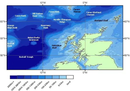
[image:31.595.92.538.172.486.2]the isolated seamounts and offshore banks; and (iii) Faroe-Shetland Channel waters.
Figure 1.1 – West coast of Scotland survey area including GEBCO topography.
1.4.1 Shelf waters
The area around the Inner Hebrides covers all of the coastal islands and water
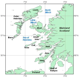
between the Scottish mainland and the Outer Hebridean islands of Barra to the south
and Lewis to the north (Figure 1.2). This is a tidally and topographically complex
region, with three main water masses: (i) an inflow of Atlantic water travelling
northwards from along the west coast of Ireland: the ‘Atlantic intrusion’; (ii) Irish sea
inflow through the North Channel between the Mull of Kintyre and Ireland; (iii)
coastal water with a lower salinity due to the high freshwater runoff from the
Figure 1.2 – Inshore waters off the west coast of Scotland
The Atlantic inflow brings high salinity, high nutrient warm water into the Sea of
Hebrides causing cyclonic circulation within the Sea of Hebrides. The Islay Front is
formed where the Atlantic water meets the Irish Sea water (Simpson et al. 1979).
Because the tides from the Atlantic and Irish Sea are 180º out of phase with each other
they cancel each other out and the tidal range is at a minimum where the two currents
meet. Gillibrand et al. (2003) showed the existence of a strong southerly flow at
depth through the Little Minch during spring, bringing with it high levels of nutrients.
The combination of the Atlantic intrusion and the southerly flow through the Little
Minch, makes the Sea of Hebrides a nutrient rich, and hence productive area.
Moreover, Gillibrand et al. (2003) also showed high levels of productivity especially
in autumn and spring around the coastline where there was high freshwater input from
the land.
1.4.2 Rockall Trough
The waters of the Rockall Trough are composed of two main bodies: the surface
(LSW). The NENAW brings warm salty waters from the south (Ellett & Martin
1973; Holliday 2003) mainly along a 50km wide band along the Scottish shelf edge
(Shelf Edge Current), over the Wyville Thompson Ridge, along the Shetland side of
the Faroe-Shetland Channel and into the Norwegian Sea (New & Smythe-Wright
2001; Turrell et al. 1999). However, there is also a significant northward flow of
warm salty NENAW in the upper layer on the west side of the Rockall Trough
(Rockall Trough Current), which flows to the west of Anton Dohrn Seamount, and
causes anticyclonic circulation around the seamount (New & Smythe-Wright 2001).
The deep water (>1200 m) is characterised by the Labrador Sea Water, which is much
fresher than the surface NENAW water, entering the Rockall Trough at its basin
south-west of Ireland, but limited to the north of the Rockall Trough by shallowing
topography (Ellet & Martin 1973; Holliday 2003). There is therefore a permanent
deep thermocline within the Rockall Trough caused by this layering of water masses.
At the upper end of the Rockall Trough the Labrador Sea Water forms a cyclonic
gyre, mixing with the cold dense Norwegian Sea Deep Water (NSDW) that overflows
from the Wyville-Thompson Ridge (New & Smythe-Wright 2001; Turrell et al.
1999).
1.4.3 Faroe-Shetland Channel
The waters of the Faroe-Shetland Channel (FSC) are the most complex, with five
different water masses meeting in the deep channel, and resulting in a dynamic
oceanic regime (Sherwin et al. 1999; Sherwin et al. 2006; Turrell et al. 1999). The
surface water is characterised by the northward moving warm saline North Atlantic
Water (NAW), which forms the Shelf Edge Current flowing along the Scottish shelf
edge northwards. Adjacent to this water on the Faroes side of the FSC lies the
Modified North Atlantic Water (MNAW) which is NAW water that has passed
through Icelandic waters and therefore cooled and freshened before arriving from the
north travelling south over the Faroes shelf forming the majority of the FSC surface
waters. Where these two water masses meet a front is formed, which is advected into
mesoscale meanders and cold core eddies by the large currents that move the NAW
water northwards (Sherwin et al. 1999; Sherwin et al. 2006). Below this water on the
Faroe Plateau side and at depths between 400-800 m is the Arctic Intermediate Water
which is cooler and less saline than either the NAW or MNAW and mainly
on the Faroe Plateau side of the FSC is the Norwegian Sea Intermediate Water
(NSIW) which has the lowest salinity of all the bodies of water. On the Shetland shelf
side of the channel this water body mixes with the AIW water due to the shallowness
of both layers on that side of the channel. Finally, there is the deep layer below 800 m
which forms the Faroe Shetland Channel Bottom Water (FSCBW), which has varying
amounts of NSDW water (cooler but saltier than that NSIW layer) dependent on the
varying supply of water from the Greenland Sea (Turrell et al. 1999).
1.4.4 Offshore biological oceanography
Biologically, the complex hydrography makes the west coast of Scotland a productive
area, with high transport of many species of fish within the shelf current (Bartsch &
Coombs 1997; Borja et al. 2002; Ibaibarriaga et al. 2007; Shelton et al. 1997). Fronts
are formed at the shelf edge between the shelf water and warmer, saltier shelf edge
current (Mann & Lazier 2006). Shelf-edge fronts are the most biologically active type
of fronts in the ocean (Mann & Lazier 2006). The shelf edge therefore provides both
food and transport for migrating species such as salmon and mackerel (Borja et al.
2002; Shelton et al. 1997), but alsoe attracts other non-migratory shelf-edge species
such as blue whiting (Armstrong pers. comm.). The little data available for
productivity within the Rockall Trough itself suggests that the Rockall Trough Gyre
also aggregates both zooplankton (Calanus: Planque & Fromentin 1996), and fish
(blue whiting larvae: Barsch & Coombs 1997).
1.5 Monitoring species distributions using passive acoustics
Recently, passive acoustic methods have become established as an effective method
of surveying some cetacean species (Clark & Fristrup 1997; Gillespie 1997; Goold
1998; Gordon et al. 2000; Hastie et al. 2003 & 2005; Leaper et al. 1992). They are
especially useful for studying the distribution of those species that are difficult to see,
such as harbour porpoises (Bailey 2006; Gillespie & Chappell 2002; Gillespie et al.
2005, Gridley 2005), or those that spend long periods underwater, such as sperm
whales (Bailey 2006; Clark & Fristrup 1997; Fristrup & Clark 1997; Gannier & Praca
2007; Gillespie 1997; Gillespie & Chappell 2002; Gordon et al. 2000; Gridley 2005;
Hastie et al. 2003; Hastie et al. 2005; Leaper et al. 1992; Leaper et al. 2000; Lewis et
al. 2007). The merits of passive acoustic methods for understanding species