The Fe3+/2+ redox couple in liquid and solid solvents

(1)

THE FE³⁺/

_²

⁺ REDOX COUPLE IN LIQUID AND SOLID

SOLVENTS

Lynn Christie

A Thesis Submitted for the Degree of PhD

at the

University of St Andrews

1996

Full metadata for this item is available in

St Andrews Research Repository

at:

http://research-repository.st-andrews.ac.uk/

Please use this identifier to cite or link to this item:

http://hdl.handle.net/10023/15528

(2)

u

THE

REDOX COUPLE

IN LIQUID AND SOLID SOLVENTS

A thesis presented for the degree of Doctor of Philosophy

in the Faculty of Science of the University of St. Andrews by Lynn Christie, B.Sc.

September, 1995

Centre for Electrochemical

and Material Sciences

(3)

ProQuest N um ber: 10170728

INFORMATION TO ALL USERS

The quality of this reproduction is dependent upon the quality of the copy submitted.

In the unlikely event that the author did not send a com plete manuscript and there are missing pages, these will be noted. Also, if material had to be removed,

a note will indicate the deletion.

uest

ProQuest 10170728

Published by ProQuest LLO (2017). Copyright of the Dissertation is held by the Author.

This work is protected against unauthorized copying under Title 17, United States C ode Microform Edition © ProQuest LLO.

ProQuest LLO.

789 East Eisenhower Parkway P.Q. Box 1346

(4)

(5)

DECLARATION

I, Lynn Christie, certify that this thesis has been composed by myself, that it is a record of my own work, and has not been submitted in any previous application for a higher degree.

Signed: Date:

I was admitted to the Faculty of Science in the University of St. Andrews under Ordinance General No. 12 on 1 October, 1991 and as a candidate for the degree of Doctor of Philosophy on 1 October, 1992.

Signed: Date: j j ‘^'1^

CERTIFICATION

I hereby certify that Lynn Christie, B.Sc. has spent twelve terms of research work under my supervision, and that she has fulfilled the conditions of the Resolution and Regulations appropriate to the degree of Doctor of Philosophy.

Signed: Date: 2~ ^

P.O. Bruce

(6)

LIBRARY DECLARATION

In submitting this thesis to the University of St. Andrews, I understand that I am giving permission for it to be made available for use in accordance with regulations of the University Library for the time being in force, subject to any copyright vested in the work not being affected thereby. I also understand that the title and abstract will be published, and that a copy of the work may be made and supplied to any bona fide library or research worker.

(7)

(8)

Acknowledgements

Thanks must be given to my supervisor. Professor Peter Bruce, for his guidance and constructive comments throughout my Ph D years, and for giving encouragement to work with my own ideas. I would like to express my appreciation to Professor Colin Vincent and all the members of C.E.M.S., past and present, for their general good humour and stimulating discussions.

My thanks are also due to Dr. Stephen Cambell, Jim Rennie and Bob Cathcart for the design and construction of the solid state polymer cell, and other members of the technical staff at St. Andrews who have helped with many odd requests. Thanks are also due to the EPSRC and Yuasa for CASE funding.

(9)

ABSTRACT

The redox couple, in the form of Fe (II) and Fe (III) trifluoromethane sulphonate, has been investigated in several non-aqueous solvents; propylene carbonate (PC), acetonitrile (ACN), tetrahydrofuran (THF), dimethyl sulphoxide (DMSO) and dimethyl formamide (DMF), as well as in tetraethyleneglycol dimethylether, a low molecular weight liquid polyether, and poly(ethylene oxide), a high molecular weight solid polyether. It has been shown that the Fe^^^^^ couple exhibits a simple one electron transfer reaction in all cases. The influence of the solvent on the electrode kinetics of the Fe^^^^^ redox couple has been investigated with a view to identifying the factors controlling the rate of the simple electron transfer process for this redox couple. The standard apparent rate constant (ksh) in each system was determined via ac impedance spectroscopy. For studies in the solid polyether solvent a new technique has been developed involving ac impedance spectroscopy at an ultramicroelectrode. This new technique proved to be a very powerful tool in the identification of interfacial processes occurring in highly resistive media

(10)

List of commonly used symbols

A Area of electrode

C Capacitance

Cdi Double layer capacitance Ce Electrode capacitance Ct Bulk capacitance

Ci Concentration of species i

Surface concentrations of O and R

Bulk concentrations of 0 and R

Cr Concentration of reduced species Co Concentration of oxidised species Do Diffusion coefficient

Di Diffusion coefficient of species I

Dap, Ds Square of refractive index and static dielectric constant respectively

E Applied potential

Ee Equilibrium potential

E ! Standard equilibrium potential

Ep Peak potential

Effiax Potential amplitude

e elementary charge

(17)

Ef Fermi energy

E Energy

e. Static permittivity

^op Optical permittivity

e Permittivity

Bo Permittivity of free space

F Faraday Constant

G Free energy

G* Free energy of activation

I Current density

lo Exchange current density

4 Peak current density

i Current

ko Rate constant at OV vs. the reference electrode ks Standard rate constant for a redox couple

ksh Standard apparent rate constant for a redox couple

k Boltzmann constant

Ep Equilibrium constant

kj Force constant ofyth vibrational level

K Electronic transmission coefficient

X Reorganisational energy

I Length between electrodes

n Number of electrons

0 Oxidised species

(18)

q Charge

qt Bond length

R Reduced species

R Resistance

R Gas constant

Rs Solution/electrolyte resistance

Rm Electrode resistance

Rb Bulk resistance

Ru Uncompemsated solution resistance Re Electrode resistance

Ret Charge transfer resistance

T Temperature

t

Time

T/ Longitudinal relaxation time

u

Potential energy

V Sweep rate

V« Nuclear frequency factor

V Voltage

Ct) Angular frequency

Y Admittance

Z Impedance

Z ’ Real impedance

Z " Imaginary impedance

(19)

z Charge valency

(20)

Constants

Elementary charge Faraday constant Boltzmann constant

Avagadro constant Gas constant

Vacuum permittivity

e

F

k

N

R

BO

1.602177 X IQ-^^C 96485 C mol'^

1.38066 X 10'^ mol'^

(21)

CHAPTER 1 INTRODUCTION

1.1 The Importance of Electrochemistry

Electrochemistry involves chemical phenomena that are associated with charge separation which often leads to charge transfer. Charge transfer can occur homogeneously in solution, or heterogeneously at electrode surfaces. Electrochemistry is not only a subject within physical chemistry but is one which spans science from biology to chemistry to physics and materials science as the world is full of interfaces, the majority of which are charged. The goal of physics is understanding how these charges move and by putting them together into cells brings in the materials science of electrodes and the organic and inorganic chemistry of the species inside the cell.

(22)

■'I

_cr

IÎ

p- «

2?

QTQ sr

I

p-Xi

c/5

fT B' rt

CL

II

(23)

In metallurgy the stability and properties of the materials, the extraction of metals from ores dissolved in molten salts, and the separation of metals from mixtures in solution all have electrochemical aspects associated with them. Soil movements in

geology have an electrochemical base: movement of the soil depends on interactions of the double layers between colloidal particles which in turn depends on the concentration of ions which affect the field across the double layer and cause the colloidal structures upon which the soil’s consistency depends to repel each other and remain stable. The use of electrochemistry in industry is widespread. Examples of such uses include electrolysis and electrosynthesis, electrodeposition and metal finishing [1-3] and water and effluent treatment. Other examples include the production of batteries and fuel cells [4,5] which are electrochemical power sources. In biology food is converted to mechanical work by biochemical mechanisms involving electrochemical reactions. Transmission of nerve impulses, the stability of blood and macromolecules involved in biological processes all depend on electrochemistry via electrochemical charge transport and double layer interactions. Also important is the application of electrochemical methods in biology i.e.

bioelectrochemistry and the development of bioelectroanalysis [6-10] which has in turn led to biosensors [9,II].

(24)

and also Br([)nsted - Bjemim theory and ionic reaction kinetics which are expressed in

terms of Debye-Huckel theory.

The subject of electrochemistry may be divided into two sub topics: ionics and electrodics. Ionics is concerned with the behaviour of ions in solution, whilst Electrodics is concerned with the theory of charged interfaces and the conditions governing the transfer of charge across them.

1.2 Ionics

L 2.1 Electrolyte Solutions

In electrochemistry the structure of both phases on either side of the interface need to be well understood. The structure of the electrode, whether it be a metal, semiconductor etc., is mainly the domain of solid state physics. On the other hand ionics, the study of bulk electrolyte phenomena is the domain of chemistry, and electrochemists in particular. The majority of the work of ionics was completed from about 1920 to 1950 and concentrated on, for example, activity coefficients of dilute aqueous solutions, electrical conductivity in molten salts or electrostatic effects on the dissociation constants of acids and bases in aqueous solutions.

(25)

since the last century. However, the relative reactivity of water puts limitations on the potentials which can be used when looking at redox species and their electrochemical behaviour, especially if the oxidation and reduction potentials fall outside the stability window of water which is less than 2. IV. As an example of the limitations of water consider the development of high voltage (>3 V) batteries: in modem lithium battery research a completely water - free environment is required as any water present will

(26)

1.2.1.1 Solid Polymer Electrolytes

Polymer electrolytes are ionically conducting phases formed by the dissolution of salts into suitable coordinating polymers, for example poly(ethylene oxide) (PEO) [15]. There are three important criteria governing the suitability of the polymer to act as a host:

(i) the polymer molecules must have polar groups or donor atoms capable of forming coordinate bonds with the cation,

(ii) the distance between coordinate groups must be such as to maximise the polymer-cation interaction,

(iii) the polymer must be capable of adopting low energy conformations to allow multiple inter- and intra- molecular coordinations.

(27)

As polymer electrolytes are solid solvent systems, the motion of ions through the polymer complex is different to that in liquid solvent systems. All ionic motion is frozen below the glass transition temperature (Tg) of the system. Above Tg ionic motion occurs and there are three main theoretical models for motion in polymer electrolytes: the Free Volume Theory of Cohen and Turnbull [17], the Configurational Entropy Model of Adam, Gibbs and DiMarzio [18,19] and the Dynamic Bond Percolation Theory of Ratner, Nitzan and Druger [20,21].

Free Volume Theory: Cohen and Turnbull [17], Cohen and Turnbull proposed that molecular transport occurred as a result of movement of molecules into voids greater than a certain critical size formed by the redistribution of the fi'ee volume of the system. They suggested that difiusive motion would occur if another molecule jumped into the hole vacated by the first before it could return. They defined the free volume of the molecule to be equal to the volume of the molecule in its cage less that occupied by the molecule itself. For the diffusion of each molecule to be non-zero, the volume of the void had to be greater than a critical value v*. A molecule can only jump into a void if the motion of the short polymer chain fragments provides an empty hole adjacent to the molecule that is going to jump. Hence, the segmental motion of the polymer chains governs the diffusion of ions or molecules through the polymer matrix.

(28)

bonds, i.e. the motion of the polymer chain segments again governs the motion of ions: the polymer chain sections have to attain a certain configuration or array providing a site adjacent to the ion into which the ion can move.

Although the free volume or configurational entropy approaches describe adequately many of the transport properties in polymer electrolytes, they are not based on a microscopic treatment and therefore, local mechanistic information is lost. Motions of ions in polymer electrolytes is strongly dependent on segmental motion of the polymer host. Ratner, Nitzan and Druger [20,21] proposed a microscopic model to describe the transport mechanisms in polymer electrolytes: the Dynamic Bond Percolation (DBF) Theory. In this model cation motion and anion motion are

considered to be fundamentally different. Cation motion can be described as being the making and breaking of coordinate bonds with motion between coordinating sites: the whole segment of polymer coordinating the cation moves before passing on the ion. Anion motion is regarded as a hopping between an occupied site and a void that is large enough to contain the ion and this only occurs between neighbouring sites. This motion has an associated probability of hopping occurring. Due to polymer motion the configuration of the polymer is continually changing and sites involved in hopping move with respect to each other. Ions can only move to a new coordination site, or hop, if the polymer chains move to a configuration that provides a coordination site or void adjacent to the moving ion.

(29)

Following on from early studies [22] that indicated over a certain temperature range many a(T) curves followed either Arrhenius (eqn. 1) or Vogel-Tamman-Fulcher

(VTF) [23] behaviour (eqn. 2), it has subsequently been found that most polymer electrolytes show one of four patterns of behaviour for ionic motion:

Eqn. 1 Eqn. 2

Arrhenius behaviour: VTF behaviour

Do = A exp (-Ea / RT) Do = Cexp[-B/(T-To)] A is a constant C is a weakly temperature dependent Ea is the activation energy for the process constant; (C a

To is a reference temperature B is a constant

(i) VTF over observable temperature range

(ii) Arrhenius behaviour for low temperatures and VTF at higher temperatures

(iii) Arrhenius behaviour over whole temperature range falling into two regions : one with a high activation energy at low temperatures and the second with a low activation energy at higher temperatures

(iii) VTF behaviour at low temperatures and Arrhenius at higher temperatures.

(30)

occurs via local relaxation processes in the polymer chains which may provide liquid like degrees of freedom [24]. Intra- and inter- polymer transitions between ion coordinating sites, and segmental motion of the chains are believed to play a major role in the ion conduction mechanism thus bringing cations to the interfacial region. The disadvantage of this type of ionic motion however, means that division of the electroactive species to and from the interfacial region is slow when compared to liquid systems (typically three orders of magnitude slower). As the polymer electrolyte is a solid it has one more disadvantage associated with it, with respect to electrochemical studies: it has a very high bulk resistance. This along with the slower diffusion can be overcome by the appropriate design of electrochemical experiments. This is dealt with later in Chapter 3.

The advantages of polymer electrolytes over classical liquid electrolytes are: (i) There are not the leakage problems associated with liquid electrolytes, (ii) The materials are often soft and form good interfacial contact with electrodes. They can often accommodate the volume changes associated with the ion-electrode exchange process,

(iii) The materials can be produced in a variety of geometries including thin films.

(31)

L2.1.2 Solid Ceramic Electrolytes

Migration of ions does not occur to any appreciable extent in most ionic and covalent solids such as oxides and halides. In contrast, there is a small group of solids called solid electrolytes (also known as superionic conductors and fast ion conductors), that usually have a rigid framework structure, but within which one set of ions forms a mobile sublattice. Solid electrolytes contain tunnels or layers through which their mobile ions may move. In this respect solid electrolytes are intermediate between typical ionic solids, in which none of the ions can move from their lattice sites, and liquid electrolytes, in which all the ions are mobile. There are two main structural requirements for high ionic conductivity in these materials: (i) there must be empty sites available for ions to hop into and (ii) the energy barrier that ions have to overcome in order to hop between sites must be small. Like polymer electrolytes, solid electrolytes have distinct advantages over liquid electrolytes. Research into the applications of these materials, especially in the development of high energy density storage systems, has grown rapidly in recent times [4,5].

1.3 Electrodics

1.3.1 The Electrode/Electrolyte Interface

Electrodics involves the study of electrified interfaces existing between two media. Interfaces occur between two immiscible solutions, two solid materials, and an electrode and an electrolyte, whether the electrolyte is a solid or a liquid. For interfaces between an electrode and an electrolyte the most fundamental process that

(32)

occurs is electron transfer and this is at the heart of electrochemistry. Electron transfer occurs via electron tunnelling across the interface either from the electrode into the electrolyte or vice versa.

The electrochemical interface has been the topic of research for many decades, probably starting with Helmholtz in 1879 [25]. The interface in aqueous systems is well documented and relatively well understood. The interface between aprotic liquid solvent systems and electrodes, although less well understood than aqueous systems, is a rapidly moving discipline, but is still in its infancy [26-31].

When studying electrode reactions it is very important to consider the interfacial region as it is in this area where the act of electron transfer occurs, the interfacial area governing the driving force of the reaction and how it takes place. Therefore, a knowledge of the potential distribution and the position of the reactant species with respect to the electrode when electron transfer occurs is important.

(33)

two points: firstly it ignores interactions that occur further from the electrode than the first layer of adsorbed species and secondly it does not allow for any electrolyte concentration dependence.

Early in this century (1910-1913) Gouy [32] and Chapman [32] independently developed a model for the double layer in which they considered the influence of electrolyte concentration and applied potential on the double layer capacitance. The double layer was of variable thickness, the ions being free to move, and was called the diffuse double layer (figure 1.3).

In 1924 Stem [33] combined the Helmholtz and the Gouy-Chapman models. The double layer was now considered to be formed of a compact layer of ions next to the electrode followed by a diffuse layer extending into the bulk solution (figure 1.4). If the electrolyte is concentrated then the thickness of the diffuse layer is less important and the potential drop is rapid. The transition between the compact and diffuse layer occurs at the distance xh. This separation plane is known as the Outer Helmholtz Plane (OHP).

Although Stem distinguished between ions adsorbed on the electrode surface and those in the diffuse layer, the double layer theory was again modified in 1928 by Grahame [34]. Grahame developed the model to allow for the existence of specific adsorption and thus has three regions (figure 1.5). A specifically adsorbed ion loses its solvation shell and so can approach closer to the electrode surface. It can also have the same charge as the electrode or be of opposite charge. The centre of these ions

(34)

defines the Inner Helmholtz Plane {IMF). The OHP passes through the centre of the non-specifically adsorbed solvated ions and the difiuse region is outside the OHP, and, as in the Stem model, the potential varies linearly with distance until the OHP is reached then exponentially in the diffiise layer.

Although extensively covered, the stmcture of the double layer is far fi*om being well established and evaluated. The Helmholtz, Gouy-Chapman, Stem and Grahame models are all based on electrostatic considerations. Further 'chemical' models, have been developed that consider the electronic distribution of the atoms inside the electrode. The first of these models to be proposed was done so by Damaskin and Frumkin [35] and the model has been reviewed recently by Trasatti [36] and Parsons [37]. From his model, Frumkin derived a correction that allows for loss of potential across the difiuse double layer. The Frumkin correction is required when calculating the tme standard rate constant of electrode kinetics.

solution electrode

Rigid arrangement of ions

(35)

electrode

G

solution

Arrangement of ions in diffuse way

Figure 1.3 The Gouy-Chapman model for the double layer

electrode

OHP

G G

° © ®

_solution

,,

G

Arrangement of ions in compact and diffuse layer

Figure 1.4 The Stem model for the double layer

solution electrode

' OHP

IHP anion

cation water

(a) Arrangement of the ions

Figure 1.5 The Grahame model of the double layer

(36)

1.3.2 Electron Transfer

Although electron transfer is now known to be the most fundamental process in many reactions, and not only in electrochemistry, it has taken many years for an understanding of this process to be developed. At about the same time that models for the double layer were being postulated chemists were trying to understand the principles governing electrochemical reactions. At the turn of the century electrochemical cells in equilibrium were being treated thermodynamically, i.e. there was no net current passing across the interface in the cell and therefore there was no net cell reaction. The thermodynamic view was that electrochemical energy was lost or gained when an electric charge was taken around a circuit made from the electrochemical cell and its two electrode/solution interfaces. The lost or gained electrochemical energy was thought to be an algebraic sum of the potential differences in the cell multiplied by the charge transferred in the reactions at each interface. This electrochemical energy sum was then equal to the change in free energy occurring in the net chemical reaction taking place in the electrochemical cell. This thermodynamical view was postulated by Nemst in 1891.

(37)

equilibrium was suppressed in favour of the thermodynamic approach. For about 50 years on from 1910, electrochemists were in awe of the thermodynamic treatment which regarded potential as the variable dependent on current. They did not try to develop a kinetic treatment for interfacial charge transfer. For example, irreversible electrode reactions were still being treated by approximations based on reversible thermodynamics as late as 1947.

By 1950 electrochemists in America and Europe had begun to think of the immediate cause of current flowing across an interface as being the influence of an external power source which caused a change in the electric potential difference across the double layer from values corresponding to the zero current situation of equilibrium.

That is the concept of overpotential (t|). Overpotential related current densities to deviations of electric potential from values when the interface was at equilibrium, i.e.

v[ was the current provoking quantity. The thermodynamic view that equilibrium was

disturbed by the passage of electrons across the interface was finally laid to rest.

This idea of overpotential had been earlier implied by Butler in 1924 and explicitly stated by Volmer and Erdey-Gruz in 1930. However in Russia this idea had been firmly adopted by Frumkin et. al. as early as the 1930’s and 1940’s. Electrochemistry became more structural and kinetic in attitude and electrochemists began to talk in terms of molecular structure at the interface and the effect of the interfacial field on electron transfer. The kinetic interpretation of equilibrium corresponding to electrons crossing the interface at the same rates in both directions became widespread with the publication of the first book in 1961 written by Vetter on electrode kinetics.

(38)

However, the electrochemists who developed these ideas were not very discerning about the type of electron transfer; they assumed classical electron emissions where electrons were climbing over barriers to get in and out of electronically conducting phases. In the 1960’s electrochemists, considering what types of electron transfer would correspond to the ranges of rates of charge transfer observed at the metal/solution interfaces, found that classical electron emissions did not explain the differences. The theory of classical electron emission was producing rates that were many orders of magnitude smaller than those experimentally observed. Electron transfer was therefore begun to be thought of as being quantum mechanical, where the electron ‘tunnelled’ through the interface into or out of the electrode. This

quantum mechanical approach was in fact first published by Gurney in 1931 [38].

(39)

thyroid gland function as well as the origin of the biological potential etc. The basic knowledge of the electron transfer process has also led to a greater understanding of the kinetics and mechanisms of biological phenomena such as nerve impulse conduction, muscle contraction, photosynthesis, energy conversion and storage, effects of hormones and drugs, clotting of blood and many others [52].

Although the tunnelling process in electron transfer is quite well understood, the parameters influencing the rates of electron transfer are not so well understood. Many theories have been put forward to try and explain possible influences on electron transfer and although substantial progress has been made, much remains to be done. Investigation into these influences is becoming a vast research field in itself.

An important factor controlling the rate of electron transfer is the nature of the solvent in which the redox couple is dissolved. Attempts to understand the influence of the solvent have been limited by the solvent characteristics, for example high resistance and slow dififiision in a solvent can hamper any electrochemical measurements made in conventional three electrode cells where the working electrode is of normal dimensions. These problems have recently been overcome by probably the greatest advance in electrochemical techniques in recent times: the development of the ultramicroelectrode by Fleischmann et. al. [53]. An ultramicroelectrode is an electrode with at least one dimension small enough that its properties are a function of its size and most ultramicroelectrodes have radii in the range 0.5-25|im. There are many different forms of ultramicroelectrode for example disk, hemisphere, band and ring etc. Due to the reduction in size of the electrode ohmic losses that arise from the

(40)

resistance of the solvent are much reduced, and mass transport rates to and from the electrode are increased due to non-planar dijflusion. This development has allowed investigations in electrochemistry that were previously thought to be impossible.

1.4 Aims of Thesis

Shedding light on the factors influencing electron transfer is a difficult task and the work presented in this thesis tries to achieve this goal. The rates of electron transfer for the redox couple in the presence of the trifluoromethane sulphonate (triflate) anion has been studied in the following media: Acetonitrile (ACN), propylene carbonate (PC), tetrahydrofuran (THF), dimethylsulphonate (DMSO) dimethylformamide (DMF), poly(ethylene oxide) (PEO) and tetraethyleneglycol dimethylether (tetramer).

(41)

REFERENCES

1 A.T. Kuhn (éd.), Techniques in electrochemistry, corrosion an métal finishing - a handbook, Wiley, London, 1987

2 C.J. Rands in Modem bioelectrochemistry eds. F. Gutmann and H. Keyser, Plenum, New York, 1986.

3 J.P Hoare & M.L. Laboda in Modem bioelectrochemistry eds. F. Gutmann and H. Keyser, Plenum, New York, 1986

4 A.F. Sammells, J. Chem. Ed., 60, 320, 1983 5 M. Hayes, Chem. Brit., 22, 1101, 1986

6 S. Srinivasan, Yu.A. Chizmadzehav , J.O’M. Bockris, B.E. Conway & E. Yeager, (eds.). Comprehensive treatise o f electrochemistry. Plenum, New York, vol. 10, 1985

7 G. Milazzo (ed.). Topics in bioelectrochemistry and bioenergetics, Wiley, 1978

8 F. Gutmann & H. Keyser (ed.). Modem bioelectrochemistry. Plenum, New York, 1986

9 A.P.F. Turner, I. Karubi & G.S. Wilson (eds.). Biosensors, fundamentals and applications, Oxford University Press, 1987

10 G. Milazzo et.al., Experientia, 36, 1243, 1980

11 A E G. Cass (ed.), Biosensors: a practical approach, IRL Press, Oxford, 1990

12 J.P Gabano, ed. Lithium Batteries, Academic Press, 1983

13 AM. Christie, Thesis fo r PhD., University of St. Andrews, Scotland, 1995

(42)

14 E. Long Thesis fo r PhD., 1993, Liverpool University 15 C.A. Vincent, Pro. Solid State Chem., _17, 145, 1987

16 Polymer Electrolyte Reviews, vols 1 & 2 (Edited by C.A. Vincent and J.R MacCallum), Elsevier Applied Science, London and New York 1991

17 M.H. Cohen & D. Turnbull, J. Chem. Phys., 31(51 1164, 1959 18 J.H. Gibbs & E.A. DiMarzio, J. Chem. Phys., 43(11 373, 1958 19 G. Adam & J.H. Gibbs, J. Chem. Phys., 43(11 139, 1965

20 Polymer Electrolyte Reviews 1_, eds. J.R. MacCallum and C.A. Vincent, Elsevier Applied Science.

21 S.D. Druger, M.A. Ratner & A. Nitzan, Solid State Ionics, 9&10. 1115, 1983

22 M.B. Armand, J.M. Chabagno & M.J. Duclot, Fast Ion Transport in Solids, Ed. P. Vashista, J. Mundy & G.K. Shenoy, North Holland and New York,

1978

23 G.S. Fulcher, J. Amer. Chem. Soc., 8_, 3339, 1925

24 Solid Polymer Electrolytes, F.M. Gray, VCH, New York 1991 25 H.L.F. von Helmholtz, Ann. Physik, 211, 1853; 7, 337, 1879 26 E.S. Saidi, Thesis for PhD., Heriot-Watt, Scotland, 1993

27 P.G. Bruce, E.S. McGregor & C.A. Vincent, in Second International Symposium on Polymer Electrolytes (ed. B. Scrosati) Elsevier, London, pp357, 1990

(43)

29 S.R. Morrison, Electrochemistry at semiconductor and oxidised metal electrodes, Plenum, New York, 1980

30 K. Uosaki & H. Kita, Modern aspects o f electrochemistry. Plenum, New York, ed. R.E. White, J.O’M. Bockris & B.E. Conway, 18, 1, 1986

31 A. Hamnett, in Comprehensive chemical kinetics, ed. R.G. Compton, Elsevier, Amsterdam, 27, chapt. 2, 1987

32 G. Gouy, Compt.Rend., 149. 654, 1910; D.L. Chapman, Phil. Mag., 25, 475, 1913

33 O. Stem, Z. Elektrochem., 30, 508, 1924 34 D C. Grahame, Chem. Rev., 41, 441, 1947

35 B.B. Damaskin & A.N. Frumkin, Electrochim. Acta, 19, 173, 1974

36 S. Trasatti, Trends in interfacial electrochemistry, Proceedings of NATO ASI, pp 25-48, 1984

37 R. Parsons, Chem. Rev., 90, 813, 1990

38 Gurney, R.W., Proc. Roy. Soc., London A 134. 137, 1931 39 J.H. Espenson & J.R. Pladziewkz, J. Phys. Chem., 75, 1971

40 W.R. Fawcett & M. Opallo, J. Electroanal. Chem., 331. 815, 1992 41 W.F. Kinard & R.H. Phile, J. Electroanal. Chem., 25, 373, 1970 42 R.W. Murray & C.R. Leidner, J.A.C.S., 106. 1606, 1984

43 R.W. Murray, T.T. Wooster, Longmire & M. Watanabe, J. Phys. Chem., 95, 5315, 1991

44 J.R. Pladziewicz & J.H. Espenson, J.A.C.S., 95, 56, 1973

45 S. Pons, J.W. Pons, J. Daschback & D. Blackwood, J. Electroanal. Chem., 237. 269, 1987

(44)

46 I. Ruff, VJ. Fredrich, K. Demeter & K. Csulag, J. Phys. Chem., 75, 1971 47 M J. Weaver, T.T.T. Li & C.H. Brabaker jr., J.A.C.S., 104, 2381, 1982 48 Yu.V. Pleskov & Yu.Ya. Farevivh, Semiconductor photoelectrochemistry.

Plenum, New York, 1986

49 S.U.M. Khan & J.O’M. Bockris, Modern aspects o f electrochemistry. Plenum, New York, ed. R.E. White, J.O’M. Bockris & B.E. Conway, 14,

151, 1982

50 Yu.V. Pleskov, Solar energy conversion. A photochemical approach. Springer-Verlag, Berlin, 1990

51 A. Szent-Gyorgyi, Science, 161. 988, 1968

52 H. Berg in Transient techniques in electrochemistry, (D.D. Macdonald), Plenum Press, New York, 1977

(45)

CHAPTER 2 EXPERIMENTAL PROCEDURES

2.1 Preparation and Purification of Salts

2.1.1 Lithium trifluoromethane sulphonate

Li2C0 3 + 2CF3SO3H 2UCF3SO3 + H2O + CO2

The appropriate quantity of LiiCOg (Aldrich 99+%) was suspended in 100ml of distilled water. To this was added lOg of neat trifluoromethane sulphonic acid (triflic acid) (Aldrich 99+ %).The solution was stirred for 4 hours until all the carbonate had been digested by the triflic acid. The resulting solution was filtered through a fine sinter and the bulk water removed from the filtrate by rotary evaporation, yielding the hydrated salt. The hydrated salt was heated under vacuum at ISO^C for 24 hours to produce the anhydrous salt, which was then directly transferred to an mBraun dry box (argon atmosphere) after slow cooling.

2.1.2 Iron (II) trifluoromethane sulphonate

An aqueous solution of trifluoromethane sulphonic acid (lOg of neat acid in 100ml of distilled water) was slowly added to an excess of iron filings. The mixture was stirred

(46)

until a pale blue solution was obtained (approximately 6 hours). The resulting solution was then filtered through a fine sinter to remove any insoluble iron oxides or hydroxides that may have formed. The bulk water was removed fi*om the filtrate by rotary evaporation, and an hydrated salt was collected. The hydrated salt was dissolved in dried acetonitrile (see section 2.2.2) and again the bulk solvent was removed from the salt via rotary evaporation. This process was repeated twice to remove water soluble impurities. The resulting salt was dried under vacuum at 80°C

for 48 hours to produce the anhydrous salt. The salt was stored in an argon filled dry box after cooling.

2.1.2 Iron (III) trifluoromethane sulphonate

+ ^2^2 + 3FT + 2JT2O + FT

(47)

2.L4 Lithium perchlorate

Lithium perchlorate (LiC1 0 4, Aldrich 99%+) was dried by heating the salt at 160°C

for 48 hours under vacuum. After cooling slowly, the dry sample was transferred to an argon filled glove box for storage.

2.1.5 Lithium hexafluoroarsenate

Lithium hexafluoroarsenate (FMC company, electrochemical grade, ‘Lectro Salt’ anhydrous) was used as received.

2.1.6 Tetrabutylammoniumperchlorate

Tetrabutylammonium perchlorate (C1 6H3 6NCIO4, Fluka puriss electrochemical

grade) was dried for 72 hours under vacuum at 80°C, and after cooling transferred to and stored in a dry box.

2.1.7 Tetraethylammonium tetrafluoroborate

The salt ((C2H$)4N(BF4), Fluka, puriss > 99%) was dried under vacuum at 80°C

for 72 hours, then transferred to dry box after cooling.

2.1.8 Tetraethylammonium hexafluorophosphate

The salt ((C2H5)4N(PF6), Fluka, purum >98%) was dried for 72 hours under vacuum

at 80°C and stored under argon in a dry box after cooling.

2.1.9 Poly(ethylene oxide)

The polymer (Aldrich, (-CH2CH20-)n ave. molar mass 4 million) was dried under vacuum at 50^C for 48 hours and stored under argon in a dry box after cooling.

(48)

2.2 Solvent Purification

2.2.1 Tetraethyleneglycol dimethylether and Propylene carbonate

Tetraethyleneglycol dimethylether [CH3(0 CH2CH2)4 0CH3], and propylene carbonate

[C4H5O3], abbreviated in this thesis to tetramer and PC respectively (both Aldrich,

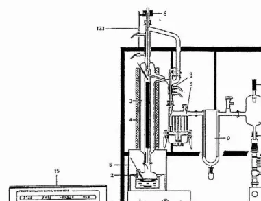
99%) were purified by vacuum distillation at 10’’ mbar using Fischer HMS 500C distillation apparatus with 90 theoretical plates (figure 2.1).

SOLVENT Bath temp. °C Mantle temp. ®C

Tetramer 147 90

Propylene Carbonate 120 57

Table 1 Temperature settings for Fischer HMS 500C when distilling solvents

(49)

[image:49.612.90.472.75.368.2]

asi

Figure 2.1. General view of the Fischer distillation apparatus HMS 500C.

Legend for Figure 2.1 ;

1 Oil bath

2 Distillation flask

3 SPALTROHR™ column 4 Heating mantle

5 Fraction collector 6 Solenoid coil 8 Distillate cooler 9 Cold trap

10 Buffer vessel 11 Vacuum line 12 Vacuum pump 13 Mounting firame 13.1 Support rod 14 Vacuum sensor

15 Distillation control device

(50)

The purity of the solvents collected was tested by cyclic voltammetry at an ultramicroelectrode. Previous attempts [1] at purification of PC reported difficulties in removing the commonly found impurity 1 , 2 propanediol sometimes produced

during distillation. 1 , 2 propanediol is formed by base catalysed ring cleavage and

hydrolysis of the cyclic carbonate during distillation. The presence of this impurity, and water results in a cathodic peak at + 1.4V vs. Lf/Li which increases in magnitude with increased concentration of each impurity. Figure 2.2 shows the cyclic voltammograms obtained for PC distilled using the Fischer HMS 500C apparatus with 90 theoretical plates (a), PC distilled using 33 theoretical plates (b) and PC as received (c). The second solvent to be distilled was tetramer the cyclic voltammogram of which is shown in figure 2.3. As can be seen fi-om figures 2 . 2 and 2.3 the solvents

produced in this way are purer than any other previously reported [1]. Neither of these solvents are electrochemically active in the potential range of the investigations carried out in this thesis.

2.2.2 Acetonitrile, Dimethyl sulphoxide and Dimethyl formamide

Small traces of water remaining in the as received solvents, despite being specified as anhydrous, {(CH3CN, Aldrich, anhydrous, 99+%); ((CH3)2SO, Aldrich, anhydrous,

99+%); (HC0 N(CH3)2, Aldrich, anhydrous, 99+%)} were removed by storing over

(51)

[image:51.612.118.435.55.600.2]

2V

(52)

-3 V

[image:52.612.174.383.62.356.2]

E vs. Pt

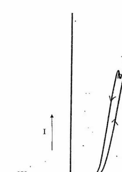
Figure 2.3 Cyclic voltammogram at a 25}o,m diameter Pt electrode for pure tetramer vs. LP/Li

2.2.3 Tetrahydrofuran

Tetrahydrofiiran {(CH2)4 0, Aldrich, anhydrous, 99.9%) was refluxed at 65-67*^0

(53)

2.3 Preparation of Polymer Electrolytes

All preparations were carried out in an argon filled dry box.

2.3.1 Cryogrinding [2]

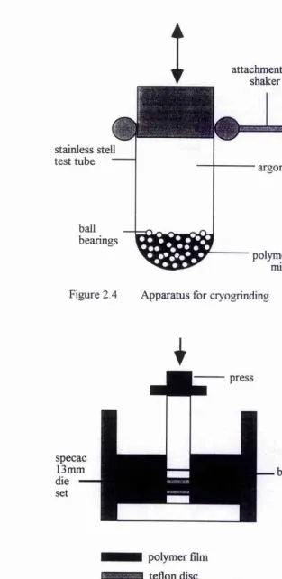
The appropriate dried salt was ground with a pestle and mortar, and a mixture of this and the PEO was transferred to a stainless steel tube containing ball bearings. The tube was sealed using a rubber bung and removed from the dry box. The whole system was then shaken for 20 minutes to half an hour with the tube dipped into a bath of liquid nitrogen. At liquid nitrogen temperatures the polymer becomes brittle and fi-actures under the action of the ball bearings. In this way an intimate, homogeneous mixture of the salt and polymer was produced. When grinding was complete the system was left to equilibrate to room temperature for 4 hours before being transferred back into the dry box. A variety of compositions of the mixture were produced by altering the proportions of salt and polymer (figure 2.4).

2.3.2 Hot Pressing

A small sample of the cryoground mixture (approx. 50 mg) was pressed at 5 tons for 30 seconds between two Teflon discs in a 13mm pellet press (figure 2.5). Under no applied pressure and using a band heater the sample was then heated to 80°C. After 4

hours of heating the sample was cooled to 35°C at which point a 2 ton pressure was applied and the sample was allowed to cool to room temperature over night. The films produced were about 1mm thick, but this thickness could be altered by using more or less sample in the first instance.

(54)

2.4 Mbraun Glove Box

The Mbraun glove box provides an inert atmosphere for all preparations that require a water and oxygen free atmosphere. Typical water levels are less than O.OSppm and oxygen levels less than 0.1 ppm. The atmosphere of the box is argon which is constantly circulated and replaced by means of a direct line to fresh cylinders of argon. The water and oxygen levels are kept to a minimum by means of sieves and copper catalysts. The sieves and catalysts are regenerated every two weeks and the box is purged with argon. Samples and apparatus entering the box do so through ports that are evacuated and then flushed with argon to remove any residual water and oxygen on their surfaces which also helps to maintain the atmosphere within the box. All polymer electrolyte preparation, including hot pressing is carried out within the box, as is the dissolution of salts for the solution systems. All prepared cells are kept within the box and electrochemical contact with these cells is via leads connected to junctions that are in turn connected to cables outside the box. This allows all electrochemical systems to remain water and oxygen free throughout all investigations.

2.5 Instrumentation

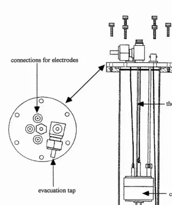
2.5.1 Polymer Cell Design

(55)

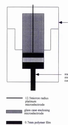
currents measured in these ultramicroelectrode studies were sufficiently small (typically less than InA) such that the platinum counter electrode also acts as a very satisfactory reference i.e. there is no need for a third electrode. The cell was then placed inside a Faraday cage before measurements were carried out (figure 2.7).

2.5.2 Liquid Cell Design

2.5.2.1 Three electrode cell configuration

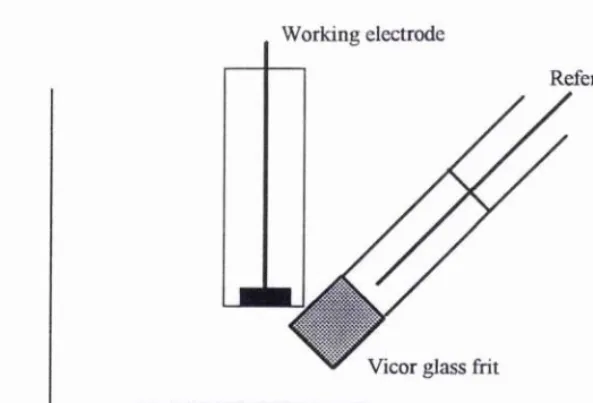
A schematic representation of the cell configuration is shown in figure 2.8. The

counter electrode is a platinum gauze (of area « 1.3 cm^) placed directly into the solution. The working electrode is a 2mm diameter platinum disc. The reference electrode consisted of a glass tube closed at the end by a Vicor glass fiit attached with heat shrinking Teflon. This glass tube contained a sample of the solution under investigation with a platinum wire placed into this. For equimolar concentrations of the redox species under investigation, the redox couple acts as its own reference with this type of reference electrode. The positioning of the working and reference electrodes within the cell is crucial. Where possible (especially for cyclic voltammetry) the tip of the reference electrode should be placed directly beneath that of the working electrode and in close proximity to it. This reduces the effects of iR drop across the cell.

(56)

2.5.2 . 2 Ultramicroelectrode cell configuration

The ceil configuration is the same as for the 3 electrode system, except that the counter electrode also acts as a reference electrode i.e. there is no need for the third electrode as the currents measured in the ultramicroelectrode are sufficiently small

(typically less than InA). The working electrode is a 25pm diameter platinum wire.

2.5.3 Electrode Polishing

All electrodes were polished with alumina of decreasing sizes (1pm, 0.3pm and

0.05pm) suspended in water on a polishing cloth (Beuhler), followed by rinsing in distilled water and thorough drying.

2.5.4 AC Impedance Spectroscopy

2.5.4.1 At an ultramicroelectrode

(57)

control of an IBM compatible PC. An ac signal of between 5 and 10 mV rms was employed in all measurements . The frequency range was 250kHz to 0.01 Hz. Data were analysed using a modified version of the complex non-linear least squares (CNLS) fitting program written by MacDonald et.al.[3].

2.5.4.2 Standard three electrode system

A Solatron 1255 Frequency Response Analyser and a 1286 Electrochemical interface were employed, under the control of an IBM compatible PC. An ac signal of between 5 and 10 mV rms was applied to the cell and measurements were taken in the frequency range 65kHz to O.OlHz. The cell was situated inside a Faraday cage and all connections were made by grounded coaxial cables. Data were analysed in the first instance using a non-linear least squares (CNLS) fitting program written by Boukamp [4] and then by a modified version of the CNLS fitting program written by MacDonald et.al.[3]

2.5.5 Cyclic Voltammetry

A Solatron 1286 potentiostat controlled by a PC-486 under software control (Corrware) was used to collect and present cyclic voltammetry data.

2.5. 6 Differential Scanning Calorimetry

All DSC scans were performed on a Perkin Elmer DSC7 differential scanning calorimeter, a 3700 data station and a TAC 7/3 instrument controller. Cryoground polymer electrolyte samples were sealed into small aluminium sample pans inside the

(58)

glove box before being transferred to the calorimeter. A sealed pan containing argon acted as a reference. For sub ambient operations, a liquid nitrogen cooler was used.

2.5.7 Powder X-ray Diffraction

Powder X-ray diffraction data was collected on a Stoe STADI/P high resolution system equipped with a linear position sensitive detector covering - 6° in 20 and

employing Ge-monochromatised Cu - K ai radiation. Data was collected in steps of

(59)

attachment to shaker

stainless stell test tube “

ball bearings

argon

[image:59.616.133.446.92.734.2]

polymer + salt mixture

Figure 2.4 Apparatus for cryogrinding

13mm _{band heater}

polymer film tetlon disc

Figure 2.5. Apparatus for hot pressing

(60)

stainless steel

current collector

12.5micron radius platinum

microelectrode glass case enclosing microelectrode

0.7mm polymer film platinum foil

[image:60.615.182.459.118.624.2]

counter/reference electrode

(61)

C I connections for electrodes

thermocouple

[image:61.616.128.482.115.536.2]

evacuation tap _cell

(62)

Working electrode

Reference electrode

Vicor glass frit

[image:62.615.170.467.72.274.2] [image:62.615.201.422.359.632.2]

Counter electrode

Figure 2 . 8 Schematic diagram of electrode configuration in liquid cell

WE CE

AMPLIFIER

IBM

Compatible PC

VGE

(63)

REFERENCES

1 S.A. Campbell, C. Bowes & R.S. McMillan J. Electroami. Chem., 284. 195, 1990

J.R. MacCallum, F.M. Gray & C.A. Vincent Solid State Ionics 18/19. 252, 1986

J.R. Macdonald, J. Scoonman & A.P. Lehner, J. Electroanal. Chem., 131. 77, 1982

(64)

CHAPTER 3 Electrochemical Methods

3.1 Cyclic Voltammetry

3.1.1 Introduction

Cyclic voltammetry is often used in the initial study of electroactive species; the data is represented in a form which allows rapid, qualitative interpretation without recourse to detailed calculation. In a typical qualitative study it is usual to record voltammograms over a wide range of sweep rates and potential limits; there may be several peaks and by looking at how these change as the potential limits and sweep rates are varied, and by noting the differences between the first and subsequent cycles, it is possible to determine how the processes represented by the peaks are related. From the sweep rate dependence of the peak height the role of adsorption, diffusion and coupled homogeneous chemical reactions may be identified. Kinetic data however, can only be accurately obtained fi*om an analysis of the first sweep. In a

cyclic voltammogram the forward and reverse sweep rates, v^nodic ^cathodic’ generally chosen to be equal, and this is the case in the present chapter and indeed the entire thesis.

(65)

electrode reaction occurs before the scan direction is reversed in order to define whether the product of the electron transfer is stable, or the reaction intermediates or the final product are electroactive. The variables are the potential limits E%, E2 and

E3, the direction of the initial sweep and the potential scan rate, v. Such a potential -

time waveform is shown below:

E

t

The potential limits define the electrode reactions that are allowed to occur. The experiment is often commenced at a potential where there is no electrode reaction i.e. i=0. To study oxidation reactions the potential is scanned in the positive direction and

to study reduction reactions the potential is scanned in the negative direction. The electrode reaction processes observed in a cyclic voltammogram depend on the sweep rate. Slow sweep rates allow slow processes to be observed whilst faster scan rates allow fast processes to be observed.

Several types of systems are studied using cyclic voltammetry:

Reversible systems are ones in which the rate determining step is that of diffusion of the electroactive species to and from the electrode, and the kinetics of the couple 0/R

(66)

(where O is the oxidised and R the reduced species) are sufficiently fast so that the electron transfer process appears to be in equilibrium at the surface of the electrode;

Irreversible systems are ones where the kinetics of the couple 0/R are poor, the rate of electron transfer is insufficient to maintain Nemstian equilibrium at the surface and therefore the rate determining step of the reaction is electron transfer. It is necessary to apply a higher potential than for a reversible reaction in order to overcome the activation barrier and allow the reaction to occur. This additional potential is called

the overpotential (t|);

It is quite common for a process that is reversible at low sweep rates to become irreversible at higher ones after having passed through a region known as quasi- reversible at intermediate values. In the quasi-reversible systems the kinetics of both the oxidation and reduction reactions make a contribution to the observed currents.

(67)

3,1 . 2 Reversible Systems

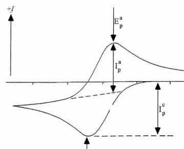
A typical cyclic voltammogram (CV) for a reversible process is shown in figure 3.1, where 0 and R are soluble species. The ratio of surface concentrations of O and R is given by the Nemst equation, and hence as the potential is swept cathodically the surface concentration of reactant must decrease, and the concentration gradient then increases. From Fick*s first law\

,V=0

tiF V dx

or

J_

nF '" A

it is expected that an increase in cathodic current follows. Due to the relaxation effect of diffusion, the concentration gradient now begins to decrease resulting in a corresponding decrease in current.

On reversing the sweep, the product R continues to be formed until the potential reaches the charge transfer equilibrium and begins to reoxidise back to O, with a corresponding anodic current flowing. The magnitude of the current increases, as before, until the surface concentration of R is depleted and the current becomes diffusion controlled. Solution of Pick's second law for species O and R, with the relevant experimental boundary conditions, reveals the exact form of the CV for a reversible process. The Randles-Sevcik equation shows that under planar diffusion control [1-3], the peak current density is

(68)

|/p| = 0.4463«f [ ^ ]

where Ip is the peak current for either the cathodic or anodic process, v is the sweep

rate and c f is the bulk concentration of species /. Thus, it is evident that a plot of Ip

against should be linear and pass through the origin for such a reversible process.

The reversible region is generally recognised to have [4]: ks > 0 . 3 cm s"^ (where k, is the standard rate constant of the redox couple).

T Æp = Ep^-Ep^ = 59lnmN

2. \Ep- Ep/2 I = 59/« mV

3. = 1

4. Ipccv"^

^ • Ep is independent of v

^ At potentials beyond Ep, T^ oc t

Table 3.1 Diagnostic tests for cyclic voltammogram of reversible processes at

(69)

[image:69.615.96.456.63.353.2]

Figure 3.1 Typical cyclic voltammogram for a reversible process, for the

reaction O + e R. Initially there is only O present in solution before sweeping cathodically.

5.1.3 Irreversible Systems

The solution to Pick's second law for the peak current density of a totally irreversible system is given by [3]

141 = 0-282 / (RT)‘'^] n(a,n^‘‘^

(70)

where «q, is the number of electrons transferred up to, and including, the rate determining step. The peak current density is therefore a function of the square root of the sweep rate, as in the reversible case. A reverse peak is absent in a totally irreversible system, although the lack of anodic wave may also be due to a fast

following chemical reaction. In the reversible case Ep is independent of sweep rate,

but for the irreversible case Nicholson & Shain [3] have shown that Ep varies with

the sweep rate according to:

Eg = ; r - - ^ : ^ i o g y 2 aerial'

where K = E Î

---acria F 0.78- — log 2 ^

actlaFD

Thus, as the sweep rate increases, the cathodic peak shifts to more negative potentials. The irreversible region is generally recognised to have [4]: ks < 2 x 10'^

cm

1. No reverse peak

2. Ip(= oc

3. Ep shifts -30/otcna mV for each decade increase in v

4- \Ep- Ep/2 1 = (48/cKcM«) mV

(71)

i. 1.4 Quasi Reversible Systems

Quasi-reversible systems are ones in which the relative rate of the electron transfer with respect to that of mass transport is insufficient to maintain Nemstian equilibrium at the electrode surface. The extent of irreversibilty increases with increasing sweep rate while at the same time there is a decrease in peak current relative to the reversible case and an increasing separation between anodic and cathodic peaks. The quasi-

reversible region is generally recognised to have [4] 0.3v‘^ > ks > 2 x 10'^ cm s"\

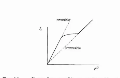
A plot of Ip as a function of readily shows the change from reversible to quasi reversible and then to irreversible behaviour (figure 3.2).

reversible.'

4

[image:71.616.83.480.357.615.2]

irreversible

Figure 3.2 Change from reversible, to quasi-reversible, to irreversible behaviour.

Kinetic data such as the rate constant are normally obtained from AEp values [5]. Working curves have been constructed of nAEp as a function of the variable q> defined by

(72)

_ (RTf^k^

(nFDjcv^'^

By comparing experimental AEp values with the working curve for several sweep rate

values the standard rate constant is readily obtained.

1. I Ip I increases with but is not proportional to it

2. I / / / i f I = 1 provided occ = aA = 0.5

AEp is greater than 59In mV and increases with increasing v

Ep^ shifts negatively with increasing v

Table 3.3 Diagnostic tests for quasi-reversible processes at 25°C

3.1.5. Systems with Adsorption

Consider the following reactions for a reversible electron transfer process where both the solution and adsorbed species are electroactive:

Osoln “• O ads

O + ne R

Rsoln ' Rads

(73)

exhibit symmetric shaped peaks corresponding to the reactions of the adsorbed species. A strong reactant adsorption gives rise to a post-peak, and a strong product adsorption gives rise to a pre-peak. The separation between the solution and the adsorption peaks reflects the strength of the adsorption, i.e. as the adsorption reduces so to does the peak separation. For weak adsorbates the peak separation is not discernible, but the voltammogram is distorted as shown in figure 3.3 [6].

E-E^IV

Figure 3.3 Cyclic voltammogram for weakly adsorbed species (b) compared to a cyclic voltammogram where no adsorbed species are present (a)

(74)

3. J. 6 Experimental Problems Associated with Cyclic Voltammetry

Double Layer Charging Ejfects

In addition to the Faradaic current (the current due to the electrochemical reaction),

there is a double layer charging current contribution given by Ui = Cdiv where I total =

Iparadaic + Dh V IS the sweep rate and Q/ is the double layer capacitance. Whilst

Iparadaic is proportional to I^i is proportional to v. C^i is usually between 2 0 and

40pF cm"2, therefore at 100 mV s~^ I^i will be between 2 and 4 pA cm“^ and this is usually small by comparison with the Faradaic current. However, at 100 Vs“l, increases to between 2 and 4 mA cm"^ and is no longer negligible. Thus, the double layer charging current distorts the voltammograms at high sweep rates, and if Q// varies over the potential range the effect is worse. This effect imposes one of the major limitations on the maximum value of the sweep rate. A good approach to eliminate the problem of the double layer charging current is to use an ultramicroelectrode (discussed later). Another method is to subtract the double layer charging current from the I-E curve for the test solution without the electroactive species (assuming the double layer/potential curve is unchanged by the presence of the electroactive species).

Uncompensated Solution Resistance

(75)

therefore be taken to ensure iR^ drop is not affecting the system under study, or is at least minimised, before performing the experiment. This may be done by incorporating a Luggin capillary or an ultramicroelectrode into the cell or by electronically applying iRu compensation during the experiment.

3.2. AC Impedance Spectroscopy

3.2.1 Introduction

Alternating current techniques have a long and well documented history within electrochemistry and several reviews have appeared over the years [7-10].

In this section a description of the ac experiment will be given as well as the definition of the impedance of a cell. This will be followed by a discussion of the ac response of some simple circuits which lead directly to an understanding of the ac response of cells.

3.2.2 The Experiment

A small amplitude, sinusoidal voltage is applied to the cell, and the sinusoidal current passing through the cell as a result is determined. To measure the impedance of a cell, two parameters are required to relate the flowing current to the applied potential. One of these parameters is analogous to the resistance in dc measurements, and equal to VntaxI Imax'

The Fe3+/2+ redox couple in liquid and solid solvents

THE FE³⁺/

²

⁺ REDOX COUPLE IN LIQUID AND SOLID

SOLVENTS

Lynn Christie

A Thesis Submitted for the Degree of PhD

at the

University of St Andrews

1996

Full metadata for this item is available in

St Andrews Research Repository

at:

http://research-repository.st-andrews.ac.uk/

Please use this identifier to cite or link to this item:

http://hdl.handle.net/10023/15528

THE

REDOX COUPLE

IN LIQUID AND SOLID SOLVENTS

uest

DECLARATION

CERTIFICATION

LIBRARY DECLARATION

Acknowledgements

ABSTRACT

TABLE OF CONTENTS

List of commonly used symbols

t

u

Constants

CHAPTER 1

INTRODUCTION

1.1 The Importance of Electrochemistry

■'I

IÎ

I

II

1.2 Ionics

1.3 Electrodics

G

G

G

G

G

G

G

G G

° © ®

,,

G

1.4 Aims of Thesis

REFERENCES

CHAPTER 2

EXPERIMENTAL PROCEDURES

2.1 Preparation and Purification of Salts

2.2 Solvent Purification

2V

2.3 Preparation of Polymer Electrolytes

2.4 Mbraun Glove Box

2.5 Instrumentation

REFERENCES

CHAPTER 3

Electrochemical Methods

3.1 Cyclic Voltammetry

3.2. AC Impedance Spectroscopy

_²