The progenitors of present day massive red galaxies up to z ap 0 7 finding passive galaxies using SDSS I/II and SDSS III

The progenitors of present-day massive red galaxies up to

z

≈

0

.

7 –

finding passive galaxies using SDSS-I/II and SDSS-III

Rita Tojeiro,

Will J. Percival,

David A. Wake,

Claudia Maraston,

Ramin A. Skibba,

Idit Zehavi,

Ashley J. Ross,

Jon Brinkmann,

Charlie Conroy,

Hong Guo,

Marc Manera,

Karen L. Masters,

Janine Pforr,

Lado Samushia,

Donald P. Schneider,

Daniel Thomas,

Benjamin A. Weaver,

Dmitry Bizyaev,

Howard Brewington,

Elena Malanushenko,

Viktor Malanushenko,

Daniel Oravetz,

Kaike Pan,

Alaina Shelden,

Audrey Simmons

and Stephanie Snedden

1_{Institute of Cosmology and Gravitation, Dennis Sciama Building, University of Portsmouth, Burnaby Road, Portsmouth PO1 3FX} 2_{Astronomy Department, Yale University, PO Box 208101, New Haven, CT 06520, USA}

3_{Steward Observatory, University of Arizona, 933 N. Cherry Avenue, Tucson, AZ 85721, USA}

4_{Department of Astronomy and CERCA, Case Western Reserve University, 10900 Euclid Avenue, Cleveland, OH 44106, USA} 5_{Apache Point Observatory, PO Box 59, Sunspot, NM 88349-0059, USA}

6_{Harvard–Smithsonian Center for Astrophysics, Cambridge, MA 02138, USA} 7_{SEPnet, South East Physics Network (www.sepnet.ac.uk)}

8_{NOAO, 950 N. Cherry Avenue, Tucson, AZ 85719, USA}

9_{Department of Astronomy and Astrophysics, The Pennsylvania State University, University Park, PA 16802, USA} 10_{Institute for Gravitation and the Cosmos, The Pennsylvania State University, University Park, PA 16802, USA} 11_{Center for Cosmology and Particle Physics, New York University, New York, NY 10003, USA}

Accepted 2012 April 25. Received 2012 April 25; in original form 2012 February 27

A B S T R A C T

We present a comprehensive study of 250 000 galaxies targeted by the Baryon Oscillation Spectroscopic Survey (BOSS) up toz≈0.7 with the specific goal of identifying and charac-terizing a population of galaxies that has evolved without significant merging. We compute a likelihood that each BOSS galaxy is a progenitor of the luminous red galaxies (LRGs) sample, targeted by SDSS-I/II upz≈0.5, by using the fossil record of LRGs and their inferred star formation histories, metallicity histories and dust content. We determine merger rates, lumi-nosity growth rates and the evolution of the large-scale clustering between the two surveys, and we investigate the effect of using different stellar population synthesis models in our conclusions. We demonstrate that our sample is slowly evolving (of the order of 2±1.5 per cent Gyr−1_{by merging) by computing the change in weighted luminosity-per-galaxy between}

the two samples, and that this result is robust to our choice of stellar population models. Our conclusions refer to the bright and massive end of the galaxy population, withMi0.55−22

andM_∗ 1011.2_M

, corresponding roughly to 95 and 40 per cent of the LRGs and BOSS galaxy populations, respectively. Our analysis further shows that any possible excess of flux in BOSS galaxies, when compared to LRGs, from potentially unresolved targets atz≈0.55 must be less than 1 per cent in ther0.55 band (approximately equivalent to thegband in the rest frame of galaxies atz=0.55). When weighting the BOSS galaxies based on the predicted properties of the LRGs, and restricting the analysis to the reddest BOSS galaxies, we find an evolution of the large-scale clustering that is consistent with dynamical passive evolution, assuming a standard cosmology. We conclude that our likelihoods give a weighted sample that is as clean and as close to passive evolution (in dynamical terms, i.e. no or negligible merging) as possible, and that is optimal for cosmological studies.

Key words: surveys – galaxies: evolution – cosmology: observations.

_{E-mail: [email protected]}

2012 The Authors

1 I N T R O D U C T I O N

The Baryonic Oscillation Spectroscopic Survey (BOSS), part of the Sloan Digital Sky Survey III (SDSS-III), is an ambitious galaxy redshift survey which will determine the expansion rate of the Uni-verse up toz≈0.7 by measuring the baryonic acoustic oscillations (BAO) and redshift–space distortions (RSD) in the galaxy power spectrum (Eisenstein et al. 2011). At the end of the 5-year observing programme, BOSS will have mapped 1.5 million massive galaxies in 10 000 deg2_{of sky, resulting in unprecedented volume and galaxy} density. Forecasts indicate that BOSS will yield measurements of the redshift–distance relationdA(z) and of the Hubble parameter

H(z) to 1 and 1.8 per cent atz=0.35 and 1 and 1.7 per cent at

z=0.55, respectively (at the 1σconfidence level; Eisenstein et al. 2011). Using one-third of the data, Reid et al. (2012) placed initial constraints onH(z=0.57) anddA(Z=0.57) at the 2.8 and 4.8 per cent levels respectively, whereas Anderson et al. (2012) constrained DV(z=0.57)≡[cz(1+z)2dA2H−

1_]1/3_{to 1.7 per cent. To achieve} the survey’s ambitious goals, systematic uncertainties in the data, modelling and methodology must be kept to a minimum, and be understood as best as possible (see Ross et al. 2011b, 2012 for a study on data systematics in BOSS).

A source of uncertainty in the modelling and measurement of the BAO is galaxy bias. Different populations of galaxies relate differently to the underlying matter density field, yielding different biases and often different scales that mark the regime over which a linear, deterministic and scale-invariant bias model is applicable. To a certain extent one can parametrize over this uncertainty, but none the less an interesting question remains concerning how much gain is possible if the bias modelling and evolution with redshift were well understood.

The best candidate for a population of galaxies with a well-understood bias evolution is a population that has been evolving with no or very little merging: the bias evolution is easily mod-elled using the Fry (1996) formalism (see also Tegmark & Peebles 1998). Massive red galaxies are the prime candidates for such a population – they are composed mostly of old stellar populations (e.g. Maraston et al. 2009), and their growth via merging since a redshift of 2 has been constrained to be small (<10 per cent) even if strictly non-zero (e.g. Wake et al. 2008). Halo-modelling analyses of massive red galaxies have repeatedly revealed a highly biased population (b≈2) with a low satellite fraction (5–10 per cent of galaxies are satellites; see e.g. Zehavi et al. 2005a; Wake et al. 2008; Zheng et al. 2009; White et al. 2011), confirming their suitability for cosmological studies. Departure from a pure passive dynamical evolution history has been shown to have a dependence on luminos-ity and colour (Tojeiro & Percival 2010; Tojeiro et al. 2011), and this opens up the possibility of weighting galaxies appropriately, so as to maximize the contribution of those that are more likely to have been passively evolving, and minimize the contribution of those that are less likely to have done so. The SDSS-I/II survey targeted luminous red galaxies (LRGs) using a mix of colour and luminosity selection cuts such as to follow the evolution of a pas-sively evolving population of stars. BOSS targeting, however, is much less restrictive in terms of luminosity and colour (especially atz>0.45; see Section 2). It is therefore not true that one population is automatically composed of the evolved products from the other. One of the goals of this paper is to identify, in BOSS, the most likely progenitors of lower redshift SDSS-I/II LRGs, and design a set of weights that allow a selection of the galaxies that are linked by the same evolutionary history.

Our other major goal is to place quantitative constraints on the formation and recent evolution of present-day LRGs, which in broad terms constitute a subset (at large luminosities or stellar masses) of what are typically called early-type galaxies (ETGs). Efforts to-wards understanding ETGs and their evolution can be split into two categories: those that focus on their stellar content, and those that primarily aim to constrain their dynamical evolution or merging history. Studies have been performed based on (see also references within): the mass or luminosity function of central galaxies (Wake et al. 2006; Brown et al. 2007; Faber et al. 2007; Cool et al. 2008) and of their satellites (Tal et al. 2012); colour–magnitude diagram (Cool et al. 2006; Bernardi et al. 2011); photometry spectral en-ergy density (SED) fitting (Kaviraj et al. 2009; Maraston et al. 2009); absorption line fitting to individual galaxies’ spectra (Trager et al. 2000; Thomas et al. 2005, 2010; Carson & Nichol 2010) or to stacked spectra (Eisenstein et al. 2003; Graves, Faber & Schi-avon 2009; Zhu, Blanton & Moustakas 2010); full spectral fitting (Jimenez et al. 2007); close-pair counts (Bell et al. 2006; Bundy et al. 2009) and clustering (Zehavi et al. 2005a; Masjedi et al. 2006; Sheth et al. 2006; Conroy, Ho & White 2007a; White et al. 2007; Brown et al. 2008; Masjedi, Hogg & Blanton 2008; Wake et al. 2008; De Propris et al. 2010; Tojeiro & Percival 2010). There is general agreement in the overall picture: ETGs constitute a uniform population of galaxies, are dominated by old and metal-rich stel-lar populations, their mean ages (either mass- or light-weighted) decrease with luminosity, and the most luminous occupy the more dense environments. There is, however, an increasing amount of evidence pointing towards some amount of recent star formation in intermediate-mass ETGs (see e.g. Kaviraj et al. 2007; Schawinski et al. 2007; Salim & Rich 2010). This amount of star formation is not in conflict with the hierarchical model of structure formation, and Kaviraj et al. (2011), through evidence coming from small mor-phological disruptions in early-type galaxies, argue that it can be explained from the contributions from minor mergers.

On the clustering side, halo modelling is rapidly being estab-lished as a successful tool to learn about galaxy formation (see e.g. Zehavi et al. 2005b; Zheng, Coil & Zehavi 2007; Ross & Brunner 2009; Skibba 2009; Skibba & Sheth 2009; Zheng et al. 2009; Ross, Percival & Brunner 2010; Tinker & Wetzel 2010; Wake et al. 2011, and references within). It is a powerful approach that connects galaxies with the dark matter haloes in which they reside, and which describes the distribution of a population of galaxies in terms of centrals and satellites, as well as their relative ratio, as a function of halo mass (which is well correlated with luminosity, see e.g. Swanson et al. 2008; Cresswell & Percival 2009; Ross, Tojeiro & Percival 2011a). For example, Zheng et al. (2007) use luminosity-dependent galaxy clustering at different epochs and the expected growth of dark matter haloes to infer a growth due to star formation betweenz=1 and the present day, after roughly taking into account growth due to the merging of centrals and satellites. This type of description of galaxy assembly can then be directly compared to predictions from semi-analytical simulations (see Zehavi, Patiri & Zheng 2012).

More specifically, the dynamical passive model can be directly tested by a halo model type of analyses. By performing halo oc-cupation distribution (HOD) modelling at two different redshifts, one can evolve the best-fitting halo model fitted at one redshift to another, assuming passive evolution. Comparison of the best-fitting halo models provides an insight about the dynamical evolution of the sample, particularly in terms of satellite accretion and disrup-tion. For most of the samples chosen, analyses show that a purely

2012 The Authors, MNRAS424,136–156

passive model would predict too many satellites at low redshift, and therefore some galaxies must merge or be disrupted (see e.g. Conroy et al. 2007a; White et al. 2007; Zheng et al. 2007; Brown et al. 2008; Seo, Eisenstein & Zehavi 2008; Wake et al. 2008). Measurements of merger rates of massive galaxies vary significantly (see table 4 in Tojeiro & Percival 2010 for a summary), but luminosity growth via merging seems confined to something between 3 and 20 per cent sincez≈1.

It seems increasingly likely that the assembly history of massive galaxies is inexorably linked to the existence of intracluster light (ICL) – a diffuse and scattered stellar component that can account for 10–50 per cent of the stellar mass in clusters (see e.g. Feldmeier et al. 2004; Mihos et al. 2005; Purcell, Bullock & Zentner 2007; Yang, Mo & van den Bosch 2009). A likely mechanism of its formation is the disruption of satellite galaxies when haloes merge (see e.g. Conroy, Wechsler & Kravtsov 2007b; Purcell et al. 2007; White et al. 2007; Yang et al. 2009, and discussions therein). A lack of conservation of light, or stellar mass, in galaxy mergers has implications for the interpretation of the evolution of the luminosity function and inferred merger histories. The fraction of light lost by a merging satellite to the intracluster medium (ICM) remains largely unconstrained, with estimates at the large halo mass end from the studies cited above varying between 15 and 80 per cent. In the present work, we make no explicit allowances for the loss of light to the ICM when two galaxies merge, but we will argue that our results are robust to this effect, within the limitations of the models and data.

In the work presented here, we approach the problem of galaxy assembly from a new direction, opposite in ethos to that of Zheng et al. (2007). We will use state-of-the-art modelling of the stel-lar evolution of a sample of galaxies to directly quantify growth from star formation, and from that infer a galaxy-merger history. We compute a model for the stellar evolution of SDSS-II LRGs by decomposing their spectra into a series of star formation and metallicity histories, as well as dust content. This allows us to make predictions of their colour and magnitudes at any redshift. This information, when combined with the target selection information for BOSS galaxies, constrains the regions in colour and magnitude space in BOSS within which progenitors of LRGs are more likely to reside. We then compute a set of weights that depend on the predicted evolution of each galaxy across the two surveys, and up-weight the objects that are more likely to be in both samples. The analysis we present depends on underlying assumptions about stel-lar evolution, initial mass functions (IMFs) and dust modelling. We perform the full analysis using two different sets of assumptions, so as to give the reader an idea of the dependence our final results on this type of uncertainty.

Isolating the likely progenitors of LRGs in BOSS is in itself no test of the merging history of the sample. Following on from our analyses in Tojeiro & Percival (2010, 2011), we test the evolu-tion in the number and luminosity density of the galaxies between LRGs and BOSS, as a way to measure the amount of merging or luminosity growth between the two redshift surveys. We also use a luminosity-weighted two-point correlation function to further test the dynamical passive hypothesis – weighting the galaxies by lu-minosity produces a clustering statistic that, on large scales, is less sensitive to galaxies within the sample merging.

This paper is organized as follows. in Section 2 we describe our two data sets, including targeting; in Section 3 we explain how we compute a stellar evolution model that describes the stellar evolution of all galaxies and spans a redshift range between 0.23 and 0.7; in Section 4 we use this stellar evolution model to compute a set of

weights that allows us to construct optimal samples of galaxies at different redshifts and explore the evolution of LRGs in the BOSS volume; in Section 5 we compute merger rates and average luminosity growth across the samples and, in Section 6, we compute the large-scale clustering of each of our samples and compare to predictions from a purely passive model. Finally, we discuss and summarize our conclusions in Section 7. Where required we assume a flatcold dark matter (LCDM) cosmology withm = 0.266, =0.734 andH0=71 km s−1Mpc−1.

2 DATA

The SDSS has imaged over one quarter of the sky using a dedicated 2.5-m telescope in Apache Point, New Mexico (Gunn et al. 2006). For details on the hardware, software and data reduction, see York et al. (2000) and Stoughton et al. (2002). In summary, the survey was carried out on a mosaic CCD camera (Gunn et al. 1998) and an auxiliary 0.5-m telescope for photometric calibration. Photometry was taken in five bands:u, g, r, iandz(Fukugita et al. 1996), and magnitudes corrected for Galactic extinction using the dust maps of Schlegel, Finkbeiner & Davis (1998). BOSS, a part of the SDSS-III survey (Eisenstein et al. 2011), has mapped an additional 5200 deg2 of southern galactic sky, increasing the total imaging SDSS footprint to nearly 14 500 deg2_{, or just over one-third of the celestial sphere.} All of the imaging was re-processed and released as part of SDSS Data Release 8 (DR8) (Aihara et al. 2011).

In SDSS-I/II, LRGs were selected for spectroscopic follow-up ac-cording to the target algorithm described in Eisenstein et al. (2001), designed to follow a passive stellar population in colour and ap-parent magnitude space. In this paper, we analyse the latest SDSS LRG spectroscopic sample (DR7; Abazajian et al. 2009), which includes around 180 000 objects with a spectroscopic footprint of nearly 8000 deg2_{and a redshift range of 0.15<z<0.5. In} SDSS-III, the BOSS target selection extends the SDSS-I/II algorithm to target fainter and bluer galaxies in order to achieve a galaxy number density of 3×10−4_h3_Mpc−3_{and increase the redshift range out} toz≈0.7. The spectroscopic footprint of the BOSS data used in this sample covers almost 3500 deg2_{of sky, and corresponds to the} upcoming DR9, which will mark the first spectroscopic data release of BOSS.

The targeting algorithms make use of five different definitions of magnitudes as follows:

(i) SDSS uber-calibrated model magnitudes (Padmanabhan et al. 2008), computed using either an exponential or a DeVaucouleurs light profile fit to therband only, denoted here with the subscript ‘mod’;

(ii) cmodel magnitudes, computed using the best-fitting linear combination of an exponential with a DeVaucouleurs light profile fitted to each photometric band independently, and denoted here with the subscript ‘cmod’;

(iii) point-spread function (PSF) magnitudes, denoted with the subscript ‘psf’, and computed by fitting a PSF model to the galaxy; (iv) Petrosian magnitudes, computed from the Petrosian flux (the flux measured within twice the Petrosian radius, in turn defined using the surface brightness of the galaxy; see Petrosian 1976; Strauss et al. 2002), and denoted here by the subscript ‘p’; and finally

(v) fibre magnitudes, computed within a 2-arcsec aperture, and denoted by the subscript ‘fib2’.

In SDSS-I/II, redshift LRGs were selected using two different algorithms. Cut I predominantly but not exclusively targeted lower

2012 The Authors, MNRAS424,136–156

redshift galaxies (z0.43) using the following selection criteria:

rp<13.1+c, (1)

rp<19.2, (2)

c⊥<0.2, (3)

μr,p<24.2 mag arcsec2, (4)

rpsf−rmodel>0.3, (5)

where the two colours,candc_⊥, are defined as

c=0.7(g−r)+1.2[(r−i)−0.18], (6)

c_⊥=(r−i)−(g−r)/4−0.18. (7) Model magnitudes are used for the colour cuts, and Petrosian magnitudes for the apparent magnitude and surface brightness con-straints. Note that whereas Petrosian magnitudes naturally fail to account for flux outside twice the Petrosian radii, and whereas this fraction varies as a function of galaxy type (see e.g. Graham et al. 2005), here they are simply used to define a sample of galaxies. When computing luminosity densities we always use cmodel mag-nitudes. Cut II mostly but not exclusively targets LRGs atz0.4 following

rp<19.5, (8)

c⊥>0.45−(g−r)/6, (9)

(g−r)>1.3+0.35(r−i), (10)

μr,p<24.2 mag arcsec2, (11)

rpsf−rmodel>0.5. (12)

Two separate algorithms are necessary as the passive stellar pop-ulation turns sharply in ag−rversusr−icolour plane, when the 4000-Å break moves through the filters.

In SDSS-III, galaxies at z 0.43 are predominantly but not exclusively targeted by the lowzselection algorithm, akin to Cut I above, but extended to fainter magnitudes. A lowzgalaxy must pass the following criteria:

rcmod<13.5+c/0.3, (13)

|c_⊥|<0.2, (14)

16< rcmod<19.6, (15)

where the two auxiliary colourscandc_⊥are defined as for SDSS-I/II above.

Galaxies atz0.43 are predominantly but not exclusively tar-geted by the CMASS selection algorithm, which extends the Cut II above by targeting both fainter and bluer galaxies. A CMASS galaxy must pass the following criteria:

17.5< icmod<19.9, (16)

rmod−imod<2, (17)

d_⊥>0.55, (18)

ifib2<21.5, (19)

Figure 1. Number density as a function of redshift for the LRG (red) and the CMASS (black) samples. The dashed line atz=0.45 shows our chosen hard boundary between the two surveys – we do not use any LRGs withz>

0.45 nor any CMASS galaxies withz<0.45.

icmod<19.86+1.6(dperp−0.8), (20)

where the auxiliary colourd⊥is defined as

d_⊥=rmod−imod−(gmod−rmod)/8.0. (21) CMASS objects must also pass the following star–galaxy sepa-ration cuts:

ipsf−imod>0.2+0.2(20.0−imod), (22)

zpsf−zmod>9.125−0.46zmod, (23)

unless they also pass the lowzcuts.

The CMASS selection algorithm was designed to loosely follow a constant stellar mass limit and, unlike Cut II in SDSS-II, it does not exclusively target red objects. Therefore, although both the LRG and CMASS samples are colour-selected, CMASS is a significantly more complete sample than the LRGs, especially at the bright end. In this paper we will split our data into two distinct redshift slices, with our lower redshifts slice in the range of 0.23 < z < 0.45 and our higher redshift slice in the range of 0.45<z<0.7. Our low-redshift slice consists exclusively of SDSS-I/II LRGs (Cuts I and II) and contains approximately 89 000 galaxies, and our high-redshift slice consists exclusively of SDSS-III CMASS galaxies, with over 250 000 objects. The low-redshift cut-off is motivated by our previous analysis of the LRGs that indicates that the sample is significantly contaminated at lower redshifts (Tojeiro & Percival 2011; Tojeiro et al. 2011). We do not make use of lowzgalaxies for the main analysis presented in this paper, mainly due to the fact that the volume and number density sampled by lowzcurrently lags behind that of the CMASS due to problems in target selection at the beginning of the observing run. We use lowzgalaxies only in Section 5.4, when investigating potentially unresolved targets in CMASS. Then(z) distribution of our two samples is shown in Fig. 1.

3 T H E S T E L L A R P O P U L AT I O N M O D E L L I N G We use the 124 stellar evolution models computed in Tojeiro et al. (2011) by stacking LRG spectra according to their luminosity,

2012 The Authors, MNRAS424,136–156

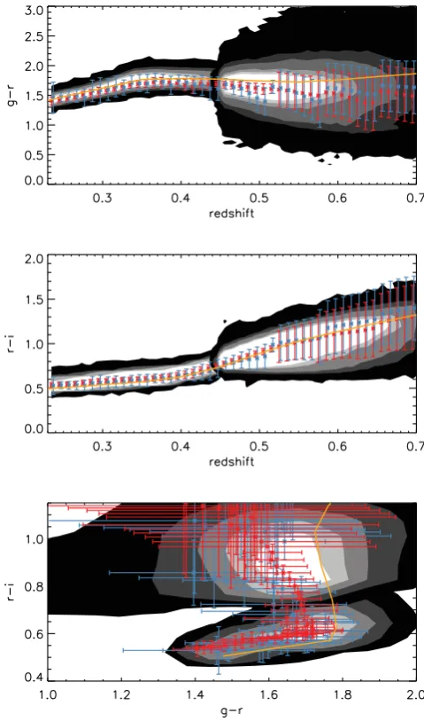
Figure 2. The observed colour evolution of CMASS galaxies contrasted with the predicted colour evolution of LRGs at CMASS redshifts. In each panel the black contours show the number density of the full LRG sample in theg−rversusr−iplane. The blue contours show the number density of CMASS galaxies for a given redshift range (given for each panel). The red dots show the predicted colours of the LRGs at the same redshifts given by the FSPS models, and the blue triangles show the predicted colours using the M11 models. The different dots correspond to the prediction of LRGs of different luminosity, colour and redshift. The solid red line shows thed_⊥=0.55 cut for reference.

redshift and colour, and subsequently analysed them with VErsatile SPectral Analysis (VESPA) (Tojeiro et al. 2007, 2009) to obtain detailed star formation histories as a function of lookback time. VESPA fits a linear combination of stellar populations of different ages and metallicities, modulated by a dust extinction, to the stacked optical spectra. Each star formation history can then be translated into a detailed evolution of any magnitude and colour with cosmic time. We have made no changes to these publicly available models other than increasing the sampling in redshift, to provide better re-solved colour and magnitude evolution.1_{We consider the solutions} obtained with two sets of stellar population models: the Flexible Stellar Population Synthesis (FSPS) models of Conroy, Gunn & White (2009) and Conroy & Gunn (2010), and the stellar popula-tion models of Maraston & Str¨omb¨ack (2011) (M11) – we refer the reader to section 4 of Tojeiro et al. (2011) for detailed information on the differences and similarities between the two sets of assump-tions, and we note that the most significant difference arises from the stellar evolution tracks.2_{One of the main results in Tojeiro et al.} (2011) is that, even though FSPS and M11 provide star formation histories that have very similar mass-weighted ages that decrease with luminosity, in the M11 case this is due to the presence of a

1_{The models from Tojeiro et al. (2011) are available at http://www.icg.}

port.ac.uk/tojeiror/lrg_evolution/

2_{Briefly, notable differences lie in the choice of the shape of the IMF,}

isochrone tracks and stellar libraries. In the case of M11, we use a combina-tion of a Kroupa (2001) IMF, the MILES stellar library of S´anchez-Bl´azquez et al. (2006) and isochrones from Cassisi, Castellani & Castellani (1997) and Schaller et al. (1992) combined with the fuel consumption approach of Renzini & Buzzoni (1986) for post-main-sequence phases. For FSPS mod-els we use a combination of a Chabrier (2003) IMF, with a MILES stellar library and the Padova isochrones of Marigo & Girardi (2007) and Marigo et al. (2008).

population of stars of young to intermediate ages (1–3 Gyr), whilst in the FSPS case this is due to a slightly younger main burst of star formation, which extends to lower ages with decreasing luminosity. These differences in the star formation histories will have an impact on the results, and we will compare results obtained using both models throughout the paper. In Section 3.1.1 we describe the star formation histories recovered with both sets of models in detail.

In Fig. 2 we show theg−randr−icolours predicted by the fits to LRGs based on the different models (red dots for FSPS and blue for M11) and how they compare to the colours of observed CMASS galaxies in four redshift ranges (blue contours). The locus of the models traces the locus of the observed galaxies remarkably well. Furthermore, the FSPS models predict a tendency to have bluer colours with increased redshift, and that is tentatively matched by the data. M11 models follow broadly the same trend, with the main differences seen atz=0.55, where M11 models predict significantly bluer galaxies (some models predict a crossing of thed⊥cut).

3.1 The composite model

The clear advantage of our set of models is that it gives a data-driven grasp on the stochasticity of the population properties. We do not need to assume that all targeted LRGs are the same and natural scatter in the colours – given by changes in metallicity and star formation rate – can be trivially accounted for. We are limited in the sense that we can only predict the evolution of any galaxy to red-shifts greater than the one it is observed at; this is because the fossil record can only hold information on thepasthistory of a galaxy. Evolving a galaxy forward requires assumptions about any subse-quent star formation, or lack of it. In order to match the samples, we need a stellar evolution model that spans the redshift range of both samples combined, and that we can use to evolve any galaxy to any redshift with minimal assumptions about their stellar evolution. We

2012 The Authors, MNRAS424,136–156

choose an approach where we compute asingleweighted composite model that spans the redshift range of the sample, based on the 124 individual stacks. At each redshift we compute a mean spectrum, weighted by the number of galaxies that make a prediction for that particular redshift (i.e. observed atz≤z). From this mean spectrum we compute a new set of magnitude and colours that define what we will call ourcomposite model. The k+E corrections of the composite model are the weighted means of the individualk+E

corrections – this composite model is therefore our best estimate of the overall average colour and magnitude evolution of the full LRG sample. Note that this approach is formally the equivalent to tak-ing the weighted mean of the 124 star formation histories for each stack, and using that weighted star formation history to recover the composite spectrum and correspondent models.

We show the colour evolution of our model in Fig. 3, and the

K + ecorrections in Fig. 4 (red for FSPS models and blue for M11). These models are used to describe all galaxies in the study: LRGs and CMASS galaxies alike. For completeness, in Section 5.5 we briefly discuss the impact of using the strictly passive stellar evolution model of Maraston et al. (2009), or the full range of 124 individual models, on our results.

3.1.1 Physical model

As mentioned in the previous section, VESPA solutions with the two different stellar population models give physical models for the galaxies that are qualitatively different, especially for LRGs atz< 0.25. FSPS produces a model that is nearly completely passive, with less than 2–3 per cent by mass in stars that are younger than 3 Gyr. M11 gives a model that sees over 90 per cent of the stellar mass formed over 12 Gyr ago (for a galaxy atz=0), but which often puts a non-negligible amount of stars at ages of 1–3 Gyr (up to 10 per cent in mass). This generates more scatter in the blue points in Fig. 2 and, as a direct consequence, a larger scatter in Figs 3 and 4.

Small but non-negligible amounts of star formation act to steepen the luminosity evolution (given by thek+Ecorrections), as the galaxy effectively ‘loses’ stars as we step back in redshift. More generally, a change ink+Ecorrections can also arise from different assumptions in the stellar evolution models, or from a different slope – or an evolving slope – of the IMF. In Tojeiro & Percival (2010) we investigated the effects of an added redshift-dependent term to thek+Ecorrections, being motivated at the time by uncertainties in the slope of the IMF. Here we will perform no such investigation, but having two models with two different slopes for thek + E

corrections provides an estimate of the impact of this uncertainty on our final results.

Both stellar population models give a constant metallicity with redshift, although M11 solutions are slightly more metal rich atZ≈

0.03, whereas FSPS prefers a solution withZ≈0.025.

Finally, the dust content is very similar in both cases – extinc-tion increases with decreasing luminosity, increasing redshift and increasing ther −icolour, varying between τV =0.2 and 0.8.

HereτVis the optical depth atλ=5500 Å and the dust extinction is

modelled according to a Charlot & Fall (2000) mixed-slab geometry (see Tojeiro et al. 2011 for full details). The weighted average, and the effective extinction for the composite model, isτV∼0.4–0.5.

3.2 K+ecorrections

We follow closely the procedure of Tojeiro & Percival (2010), which we summarize here for completeness.

Figure 3. The composite stellar evolution model, computed according to the procedure in Section 3.1. In all panels the shaded contours show the number density of LRGs (atz<0.45 and on the bottom half of the last plot) and CMASS galaxies (atz>0.45 and on the top half of the last plot). The red (blue) solid line shows our composite stellar model obtained using the FSPS (M11) VESPA star formation histories. It is a weighted average of the models shown in Fig. 2. The error bars show the 1σdispersion of the models shown in Fig. 2 in each redshift bin. For reference, the yellow line shows the LRG purely passive model of Maraston et al. (2009) – see Section 5.5.1.

Our composite model providesLλ(tage), the luminosity per unit

wavelength of a galaxy of agetage. WeK+e-correct all galaxies to a common redshift ofzc =0.55, and calculate corrected absolute magnitudes in filters shifted tozc=0.55 as

Mr0.55=rcmod−5 log10

DL(zi)

10 pc

−Ke(z, zc), (24)

with

Ke(z, zc)=

= −2.5 log10

1 1+z

TλoLλo(z)λodλo

Tλ/(1+zc)λ−

1 e dλe

Tλo/(1+zc)Lλe(zc)λedλe

Tλoλ−

1 o dλo

.

(25)

2012 The Authors, MNRAS424,136–156

Figure 4. K+ecorrections in ther0.55band (triangles) and in thei0.55band

(asterisks). The red lines refer to the FSPS models, and the blue lines to the M11 models. The error bars show the 1σscatter around the mean from the 124 individual stacks. These corrections allow us to compute the evolved absolute magnitude of any galaxy at z=0.55, in the two shifted filters (therefore for galaxies atz=0.55 this correction is fixed and independent of their spectra or modelling). The corrections in ther0.55band are steeper

because it traces the 4000 Å break at these redshifts – see Fig. 5. The scatter in the M11k+Ecorrections is larger, as these models predict stochastic events of star formation at young to intermediate ages in some of the stacks. For reference, the yellow line shows the LRG purely passive model of Maraston et al. (2009), as a dashed line for thei0.55band and as a solid line

for ther0.55band – see Section 5.5.1.

Here,λois in the observed frame andλein the emitted frame.Tλ

is the SDSS’sr-band filter response, andLλ(z) is the luminosity

density of a galaxy at redshiftz, given by the fiducial model. We also computeMi0.55, using exactly the same procedure as on the

iband. Note that for a galaxy atz=0.55, theK+ ecorrection is independent of the observed or modelled spectrum and equals −2.5 log10[1/(1+z)]. By choosingzc=0.55, roughly the peak of the redshift distribution of CMASS galaxies, we minimize the effect of the modelling on CMASS galaxies. The other option would have been tok+e-correct to median redshift of LRGs. However, as the composite stellar population model is based on the spectra of LRGs, its predictions must be at least as robust for LRGs as for CMASS galaxies, if not more so. Therefore, our procedure is the more robust approach. We show thek+ ecorrection in the rand ibands in Fig. 4. For reference, in Fig. 5 we show the expected observed-frame spectrum of a typical galaxy in the sample at zc = 0.55, alongside the three broad-band filters used in this paper.

3.3 Comparing CMASS galaxies and LRGs

We can use theK +ecorrected absolute magnitudes to broadly characterize the two samples. Fig. 6 shows a simple comparison of the magnitude distributions for both samples and their evolution with redshift computed for both therandibands. Once again, we show the results for the FSPS model in red and for the M11 model in blue. Here the only model differences come through theK + ecorrections, with the different slopes between models (shown in Fig. 4) naturally giving differentk+Ecorrected absolute magni-tudes. M11 shows a steeper slope with respect to FSPS, with the crossing point atzc=0.55. So for a galaxy atz<0.55, M11 will predict afainter k+ Ecorrected magnitude atz=0.55. In

con-Figure 5. The expected observed spectrum of a typical galaxy in the sample atz=0.55 (black). The three broad-band filters used for target selection are overplotted:gband in blue,rband in green andiband in red. For reference, we show in grey the expected observed spectrum of a galaxy atz=0.3.

trast, for a galaxy atz>0.55, M11 will predict abrighter k+E

corrected magnitude atz=0.55. By construction, the magnitudes for galaxies sitting atz=0.55 will match for both models due to our choice of filters. The top panel of Fig. 6 shows the effect of having different slopes for thek+Ecorrections – for LRGs this is about 0.3 mag in ther0.55band; for CMASS galaxies it is much smaller, at less than 0.1 mag. These values are roughly halved for thei0.55band. The bottom two panels of Fig. 6 show the evolution of the corrected magnitudes with redshift (solid contours for FSPS and line contours for M11). As expected, we see a steeper evolution with redshift using the M11 contours.

Fig. 7 displays colour–magnitude relations. Here we show only the results using FSPS models as the results are similar in both cases. The CMASS sample has a broader range in absolute magnitude and colour than the LRG sample, as expected given the larger number density. The clear trend seen between rest-frame colour andMr0.55 is explained simply by target selection. To help make this point we show the expected evolution of the colour–magnitude relation of an object at the faint end of the survey (cmodel=19.9 atz=0.45) and an observed colour ofr−i=0.8, betweenz=0.25 and 0.7 – this is the red line in both plots. Any object to the faint side of the red lines would fail the magnitude cuts in theiband of the CMASS algorithm. This gives an obvious artefact when plottingMr0.55versus colour, whereupon the CMASS selection does not select faint blue galaxies. The bright end slope is a consequence of volume effects, coupled with the slope of a typical galaxy spectrum.

4 S A M P L E M AT C H I N G

We now construct galaxy samples at high and low redshifts that are coeval according to our composite stellar evolution models. We continue to closely follow the methodology of Tojeiro & Percival (2010), which we summarize below. We have to take into account three redshift-dependent effects:

(i) the intrinsic evolution of the colour and brightness of the galaxies,

(ii) the varying errors on galaxy colour measurements and (iii) the varying survey selection function.

2012 The Authors, MNRAS424,136–156

Figure 6. ComparingK+ecorrected magnitudes in SDSS-I/II LRGs and BOSS CMASS galaxies. Top: the distribution of absolute magnitudes for LRGs (dashed lines) and CMASS galaxies (solid lines). The different colours show the results from using different stellar population models, with FSPS in red and M11 in blue. The two panels show the magnitude computed either in the rest-frameroriband. Bottom: the absolute magnitude with redshift on both samples. FSPS results are shown in the solid contours, and M11 in the line contours. The samples are split atz=0.45; we do not use any LRGs withz>0.45 nor any CMASS galaxies withz<0.45. These plots show clearly the reach to fainter magnitudes of the CMASS sample. See main text for a discussion on the effect of the stellar population models.

Figure 7. Rest-frame,k+ecorrected colour–magnitude relations for CMASS galaxies (filled contours) and LRGs (overplotted black contours), as a function ofMi0.55shown on the left-hand panel, and as a function ofMr0.55on the right-hand side. CMASS galaxies show a broader range in their rest-frameMr0.55−

Mi0.55, as well as fainter reach and median in both magnitudes. The right-hand-side plot shows a clear trend of rest-frame colour withMr0.55, with redder

colour going with lower luminosity. This is trend is a result of target selection, particularly the magnitude cut – we show the expected evolution of the colour–magnitude relation of an object at the faint end of the survey (cmodel=19.9 atz=0.45) and an observed colour ofr−i=0.8, betweenz=0.25 and 0.7. Any object to the faint side of the red lines would fail the magnitude cuts of the CMASS algorithm.

Our correction for item (i) is given by our composite stellar evolu-tion model. We include an evolving colour scatter term to allow for (ii). Tojeiro & Percival (2010) used the population scatter around the stellar evolution model with redshift. Tojeiro & Percival (2011) up-dated this term to be based on the evolution of photometric errors as a function of apparent magnitudes, which were modelled as a func-tion of redshift – see their secfunc-tion 3. The motivafunc-tion was twofold: first, the photometric errors are driven principally by the apparent magnitude of an object, rather than its redshift; and secondly this is less dependent on the choice of stellar evolution modelling. We adopt this approach here. For (iii) we construct a set of weights that ensures a given population of galaxies – in terms of colour and

absolute magnitude – is given the same weight in the high- and low-redshift samples, as described in the next section.

4.1 Weighting scheme

We use the weighting scheme of Tojeiro & Percival (2010), which keeps the total weight of eachgalaxy populationthe same in differ-ent redshift slices.

Suppose an LRG,gA, is faint and therefore can only be seen in a small fraction of the CMASS volume,fV, but can be seen in the full LRG volume. Then our weighting scheme will givegAa weight that is equal tofV. Consider now a faint CMASS galaxy that is

2012 The Authors, MNRAS424,136–156

observed infV, and whose magnitude and colour evolution matches those predicted forgA. This galaxy will by definition also only be observed in a fractionfV of the CMASS volume. Our weighting

scheme givesgBa weight on unity. Note that this is the opposite approach to the traditionalVmaxweight, which wouldup-weight gB by 1/fVand givegAa weight of unity.

Explicitly, for an LRG in a volumeVLRGwe calculate

Vmatch,i=

VLRG VLRG max,i

×min

VLRG max,i

VLRG ,V

CMASS max,i

VCMASS

, (26)

and similarly for a CMASS galaxy, in a volumeVCMASS:

Vmatch,i=

VCMASS VCMASS max,i

×min

VLRG max,i

VLRG ,V

CMASS max,i

VCMASS

, (27)

whereVmax,iis the volume a galaxyiwould have been observed

in either survey, according to the full target selection cuts and the evolution of its colour and magnitude, as given by the composite model.

Where the traditionalVmaxestimator would up-weight galaxies only visible in a fraction of the volume in which they were observed, we instead give these galaxies a weight of unity and down-weight the corresponding galaxies with the same properties as observed in the other volume.

The interpretation of theVmatch weight is different from that of the traditional Vmax weighting. Although the latter gives us the means to correct for incompleteness and yields true space densities, the former must be interpreted as a weighting scheme rather than a completeness correction. That is, Vmatch weighted number and luminosity densities are still potentially volume incomplete, but the populations are weighted in such a way that they are equally represented at both redshifts. We can compare the distribution of the total weighted luminosity for the two slices, but we cannot interpret these functions as giving the true luminosity density.

The advantage of this weighting scheme is that we sample dif-ferent populations equally based on volume, and therefore obtain a weighted population such that galaxies observed throughout a large volume are up-weighted. It also implicitly checks that we are only using populations that exist in both samples, without having to do such a test explicitly (e.g. Wake et al. 2006).

4.2 The progenitors of LRGs

A large value ofVmatch (Vmatch varies between 0 and 1) indicates that a galaxy belongs to a population that can be observed across a large fraction of both surveys, and a small value ofVmatchmeans a population of galaxies is only present in a small fraction of the volume in at least one of the surveys. In other words, the larger this value for a CMASS galaxy, the more likely this galaxy is a progenitor of a typical LRG galaxy, and vice versa.

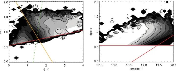
Fig. 8 shows a mapping of the average value of this weight on to the two CMASS targeting parameter spaces: ag−rversusr− iplot, and ad_⊥ versus the cmodel magnitude in theiband. We show the results using the FSPS models in the solid contours and the results using M11 in the line contours, which are qualitatively similar. The colour–colour plot shows a clear trend for the average value ofVmatch to increase to redderg− rcolours, as expected if LRGs were exclusively made of metal-rich and old stars. Inter-estingly, we also see that some blue regions of the colour–colour plot display an increase of the average value of theVmatch weight. This relation is a result of the small but significant numbers of young-to-intermediate-aged stars detected in LRG spectra at BOSS redshifts (corresponding roughly to stars aged between 1 and 3 Gyr in SDSS-I/II galaxies). The orange line in the left-hand plot of Fig. 8 shows theg−i=2.35 cut of Masters et al. (2011), which was motivated by the morphological analysis of a small subsample of CMASS galaxies withHubble Space Telescope(HST) imaging. They suggest that selecting galaxies withg−i>2.35 produces a cleaner sample of early-type galaxies (90 per cent) that are more traditionally associated with typical LRGs. Additionally, we predict that at least a fraction of the galaxies that sit in the blue end of that colour–colour plot are also LRG progenitors, temporarily visiting the blue cloud due to small amounts of star formation. Assuming that they retain their morphology (it is hard to imagine a scenario where they would not), our analysis makes quantitative predictions on the fraction of star-forming ellipticals that should be found on that part of the diagram, given the morphological mixing of the LRG sample (not currently known, to our knowledge). This result can be turned into a test of stellar population synthesis (SPS) models, as different sets of models will predict a different number density at those colours. We leave this exploration for future work.

The right-hand-side panel of Fig. 8 shows an uninterrupted trend to lowerVmatchtowards fainter magnitudes. Interestingly, the slope

Figure 8. AverageVmatchweight as a function of colours andi-band magnitude, shown for the two main targeting parameter space diagrams in CMASS.

A darker colour corresponds to a lower value ofVmatch, and the brighter colours to the regions in parameter space that have the largest likelihood of being

progenitors of the LRG sample. The red solid lines show targeting cuts. The orange line on the plot on the left shows the morphology cut derived in Masters et al. (2011), and the dashed green line shows the blue cut of the cut-II selection in Eisenstein et al. (2001).

2012 The Authors, MNRAS424,136–156

Figure 9.k+ecorrected absolute magnitudes for CMASS galaxies (black), LRGs (green) and the subset of CMASS galaxies that is seen in less than 5 per cent of the LRG volume according to our model (purple). These lie almost exclusively at the faint end, demonstrating how important the apparent magnitude cut is in the sample matching between the two surveys. Solid lines for results using the FSPS models and dashed lines for results using M11.

of theVmatchcontours is almost parallel to the sliding cut ind⊥with thei-band magnitude. This cut was designed to follow a line of constant stellar mass (Maraston et al., in preparation), suggesting thatVmatchhas a clear dependence on stellar mass, as it should.

A complementary way to examine theVmatchweights is to isolate the CMASS galaxies with a smallVmatch weight – these are the CMASS galaxies that are less likely to be the progenitors of a typical LRG. Fig. 9 shows theK+ecorrected absolute magnitude distribution of those CMASS galaxies withVmatch<0.05, i.e. that are observed in less than 5 per cent of the volumes of the surveys. We clearly see that these galaxies are well confined to the faint end of the CMASS population. The difference between the two models is a consequence of the steeper luminosity evolution given byK+ ecorrections of the M11 models – CMASS galaxies are typically brighter at LRG redshifts (when compared to a flatter luminosity evolution), and are seen through more of its volume.

Fig. 10 presents the distribution of the absolute rest-framer0.55−

i0.55colour for the same populations as in Fig. 9. The bias towards losing intrinsically redder galaxies is explained by the fact that the CMASS sample is itself biased towards redder galaxies inMr0.55−

Mi0.55at the faint end (see Section 3.3 and Fig. 7) due to thei-band selection.

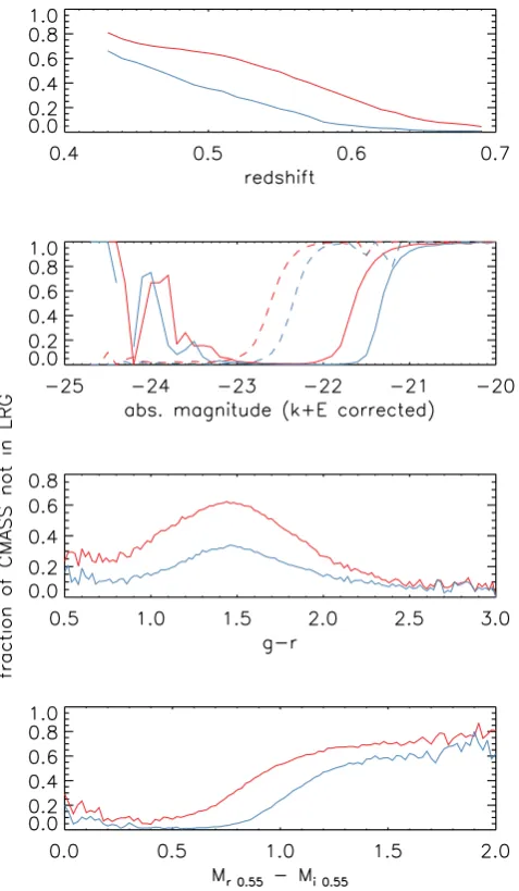
We show the fraction of CMASS galaxies that are observed in less than 5 per cent of the LRG volume as a function of redshift, absolute magnitude,g−rand rest-frameMr0.55−Mi0.55colours in Fig. 11. Once again, these figures demonstrate that magnitude is the dominant reason why these galaxies are not well matched between samples, butrest-framecolour also plays a part – see the upturn in the fraction of lost objects for brightMr0.55compared to the fraction of lost objects for brightMi0.55. These are the galaxies with redder

Mr0.55−Mi0.55rest-frame colours.

5 M E A S U R I N G P O P U L AT I O N E VO L U T I O N In order to compute merger and luminosity growth rates, we first define the samples of CMASS galaxies and LRGs to be investigated (Section 5.1). Having selected matched samples, we then study the

Figure 10. Distribution ofk+ecorrected, absoluter0.55−i0.55colours for

CMASS galaxies (black), LRGs (green) and the subset of CMASS galaxies (purple) that is seen in less than 5 per cent of the LRG volume according to our model. Solid line for results using the FSPS models and dashed line for results using M11.

evolution of a number of quantities. In Section 5.2 we consider lu-minosity functions and in Section 5.3 the rates of change in number density, luminosity density and typical luminosity per object.

5.1 Sample selection

In each survey we take the brightest objects until we reach a given

K + ecorrected absolute magnitude, and we compute a V match-weighted comoving number densitynand aVmatch-weighted lumi-nosity density. We consider the following options to define the limiting magnitude in each sample,Mmin,CMASSandMmin,LRG.

(i) A flat cut ink+Ecorrected absolute magnitude across the two surveys: in this caseMmin,CMASS=Mmin,LRG. In general,nLRG=

nCMASSandLRG=CMASS.

(ii) A cut in K + e corrected absolute magnitude such that both samples have the same comoving number density. In this case,nLRG=nCMASSby construction, but in generalMmin,CMASS=

Mmin,LRGandLRG=CMASS.

(iii) A cut inK + e corrected absolute magnitude such that both samples have the same comoving luminosity density. In this case,LRG=CMASSby construction, but in generalMmin,CMASS=

Mmin,LRGandnLRG=nCMASS. This can be advantageous in cluster-ing analyses that are luminosity weighted (see Section 6).

To avoid confusion, we will refer to the number and luminosity densities computed using a flat cut in absolute magnitude asnand , respectively.

5.2 The luminosity function

With full knowledge of the completeness of the sample, we can compute luminosity functions and study their evolution. The com-pleteness, in terms of the sample one intended to select, is primarily affected by the following well-understood effects:

(i) targeting completeness – not all objects that pass the targeting cuts are targeted due to bright star masks, fibre collisions or other tiling issues;

2012 The Authors, MNRAS424,136–156

Figure 11. The fraction of CMASS galaxies that is seen in less than 5 per cent of the LRG volume as a function of redshift (first panel), absolute magnitude (second panel – solid line forMr0.55and dashed line forMi0.55),

observedg−rcolour (third panel) andk+Ecorrected rest-frame colour Mr0.55−Mi0.55(bottom panel). Red lines for results using the FSPS models

and blue for M11.

(ii) redshift failure – not all objects with a spectrum successfully yield a redshift;

(iii) star/galaxy separation – galaxies that fail the star–galaxy separation in spite of being genuine galaxy targets.

We use the targeting completeness and redshift failure corrections as described in Percival et al. (2007) for the LRGs and in Ross et al. (2012) for CMASS galaxies; both samples have very high spectro-scopic completeness (>97 per cent). The fraction of galaxies lost to the star/galaxy separation can be estimated from commissioning data, where star–galaxy cuts are less restrictive or not included at all. This fraction is estimated to be 1 per cent for CMASS galaxies (Padmanabhan et al. in preparation), 1 per cent for Cut-II LRGs and 1 per cent for Cut-I LRGs (Eisenstein et al. 2001). This could re-sult in a systematic underestimate of the number density of CMASS galaxies compared to LRGs, which would at most be≈1 per cent. In an independent analysis, Masters et al. (2011) found 3±2 per cent of CMASS targets in the COSMOS field that failed the star–

galaxy cuts, in spite of being obviously galaxies when captured in high-qualityHSTimaging. This measurement agrees well with the numbers cited above.

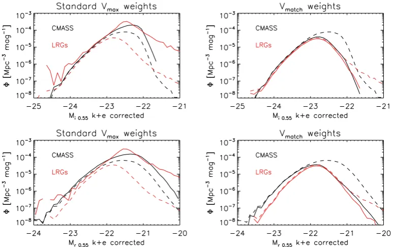
Fig. 12 presents luminosity functions weighted byVmatch (right panels) and by the standardV/Vmaxweights (left panels). For ref-erence, in both panels we show in the dashed lines the luminosity function without any completeness correction – in this case it is simply the number count of galaxies per magnitude bin, divided by the volume of each survey. We compute the luminosity function in

Mi0.55 (top) andMr0.55 (bottom) absolute magnitudes. Recall that theVmatch scheme weighs each sample such that populations are matched in terms of volume, but that it does not yield true vol-ume densities (see Section 4.1). Compared toV/Vmaxweights this

down-weightsfaint galaxies in both samples, such that the overall

luminosity functions are matched. In the case of zero merger evo-lution or contamination (and in the case of perfect modelling), our

Vmatchweights fully account for changes in thestellarevolution and the two luminosity functions should therefore match. Differences can be interpreted in a number of ways:

(i) growth (i.e. merging);

(ii) contamination: galaxies in CMASS that have identical colour and magnitudes to LRG progenitors but evolve to be something else at low redshift;

(iii) resolution issues: close pairs of galaxies failing to be re-solved in CMASS due to instrumental and atmospheric limitations; and

(iv) inadequacies in the modelling: in this case, mostly in the slope of thek+Ecorrections.

It is clear that the luminosity functions of CMASS galaxies and LRGs are better matched inMi0.55than inMr0.55. There is a larger

uncertainty in the slope of thek+Ecorrections in therband, as that traces a region of the spectrum sensitive to small amounts of star formation atzc = 0.55. Small mismatches in the amount of star formation at those redshifts between our composite model and the true star formation rate of CMASS galaxies may not be enough to down-weight them using our method, but reveal themselves in a detailed comparison such as the one we attempt here. We therefore argue that thei-band luminosity is more reliable for the purposes of our analysis, as it is a better tracer of overall luminosity, or stellar mass, of the galaxy.

Differences in the shape of the luminosity function can help identify the reasons for the differences between the two samples. We present a more quantitative analysis in the next section, where we construct three estimators to quantify differences in the amplitude and shape of the luminosity function, but first we look at the effect of using a differentk+Ecorrection model.

Fig. 13 shows the same luminosity functions as Fig. 12, but using the absolutek+Ecorrected absolute magnitudes obtained using the M11 models. The differences are substantial, especially for the LRGs. Note the differences are already apparent in the uncorrected (dashed) curves, showing the reason lies with the computation of the absolute magnitudes themselves, and not with the weighting scheme. These results are consistent with the steeperk+E cor-rection and the magnitude distributions shown in Figs 6 and 9. The effect is primarily due to thek+Ecorrected absolute magnitudes of the LRGs atzc = 0.55 – they are≈0.3 mag fainter than those predicted with the flatter FSPSk+Ecorrection. The differences are larger for the LRG magnitudes simply because of our choice ofzc, which minimizes the effect of the modelling for CMASS galaxies (see Section 3.2).

2012 The Authors, MNRAS424,136–156

Figure 12.VmatchandVmax-weighted luminosity functions in thek+ecorrectedr0.55−andi0.55bands (obtained using the FSPS composite model), for the

CMASS and LRG samples. The dashed lines show the unweighted luminosity functions. TheVmaxweights work by mostly up-weighting the fainter galaxies,

as can be seen in the two left panels. This typically breaks down for faint galaxies. TheVmatchweight, in turn, up-weights and down-weights galaxies according

to their relative presence on the other survey – this can be seen in how effectively we down-weight faint galaxies in both surveys to get a luminosity function that is well matched – particularly in thei0.55band. Poisson errors are negligible (∼1 per cent) except for the brightest or faintest half magnitudes (1–10 per

cent). See text for further discussion.

Figure 13.Same as Fig. 12, but using the absolute magnitudes computed with M11 models.

There is an overall improvement in the matching of allVmatch luminosity functions across the two surveys when using only red CMASS galaxies (withg−i>2.35) for both models. This im-provement is small, of only a few per cent, and is explained by the fact that theVmatchweights are lower for the bluer galaxies, and so they are already being down-weighted when using the full sample.

Contrasting the two weighting schemes we see that the standard

V/Vmaxweights up-weight galaxies at the faint end. Bright galaxies are visible in most of the survey and therefore incur a small cor-rection. This shifts the break of the luminosity function to fainter magnitudes when compared to the uncorrected curve, but the falling in number density after that must not be trusted completely –V/Vmax

2012 The Authors, MNRAS424,136–156

weights get increasingly dominated by Poisson error towards faint magnitudes (see Section 4.1). This is visibly the opposite than what happens using theVmatchweights in the opposite panels.

5.3 Rates of change

In order to understand the differences seen in Figs 12 and 13, we define three estimators to quantify changes as a function of magnitude. For a pair of samples matched on luminosity density, we define a merger rate as

rN=

1− nLRG nCMASS

1

t, (28)

where tis the time, in Gyr, between the mean redshift of the two samples (defined such that t>0). Similarly, for a pair of samples matched by number density, we define a luminosity growth as

r=

LRG CMASS

−1

1

t. (29)

These two rates would be exactly a merger rate and a luminosity growth in the absence of complications such as

(i) resolution issues: close pairs of galaxies failing to be resolved within instrumental and atmospheric limitations;

(ii) contamination: galaxies in CMASS not following our com-posite stellar evolution model and evolving into a different region of colour and magnitude space than that of the LRGs at low redshift;

(iii) loss of light to the ICM when a merging event occurs; and (iv) a systematic offset in the computation of the absolute mag-nitudes as a result of the modelling.

We investigate (i) in Section 5.4. Item (ii) is an intrinsic limitation of any methodology without a full understanding of the evolution of

allgalaxy types. Item (iii) can potentially be investigated by using small-scale clustering and a halo occupation distribution type of approach, in order to estimate the fraction of satellite merging and a fraction of light lost to the ICM. We do not perform such an analysis in the present paper, but we will show in Section 7 how, when taken together, the results we show in this and in the next section (large-scale clustering) present a picture that points strongly towards a small amount of population growth. To deal with item (iv), we also define a galaxy growth rate by using our samples matched by a fixed

k+Ecorrected absolute magnitude (see Section 5.1) as

rg=

1− n

LRG/LRG nCMASS/CMASS

1

t. (30)

Here,rgwould match the merger rate even in the presence of con-taminants (assuming that the luminosity function of the contam-inants was the same as the luminosity function of the CMASS galaxies). More generally, it can be interpreted as a rate of change of luminosity per single object across the two surveys. AlthoughrN

andr are dominated by the relative amplitude of the luminosity

function between the two redshifts,rgtells us about differences in the shape.

5.3.1 Results

We computerNandras a function ofMi0.55(the magnitude of the faintest LRG in the sample, which was used to compute the matched samples – see Section 5.1), which are shown in Figs 14 and 15. Our most inclusive samples (i.e. whereMi0.55= −22) include≈95 per cent of the LRGs and≈40 per cent of CMASS galaxies, and have

Figure 14.The merger rate, per Gyr, computed as per equation (28) as a function of the magnitude of the faintest LRG in the sample. The black line showsrN×100 for the full sample and the red line for galaxies withg−i>

2.35. The results obtained from using M11 models (dashed lines) show the same slope with magnitude as the results using FSPS models (solid lines), but are afactor of 2–3lower. Poisson errors shown.

Figure 15.The luminosity growth, per Gyr, computed as per equation (29) as a function of the magnitude of the faintest LRG in the sample. The black line showsr×100 for the full sample, and the red line for galaxies with g−i>2.35. The results obtained from using M11 models (dashed lines) show the same slope with magnitude as the results using FSPS models (solid lines), but are afactor of 2–3lower. Poisson errors shown.

large stellar masses with log10M/M11.2 (Maraston et al., in preparation).

Note thatrN is negative for all magnitudes, although it tends to zero towards brighter magnitudes. This implies that, for the same integrated luminosity density, there aremore LRG galaxies per comoving volume than there are CMASS galaxies. That is, CMASS galaxies appear to bebrighterthan LRGs in thei0.55band. This is expected from our analysis of the luminosity functions of Figs 12 and 13. We emphasize that if this brightening was due simply to the stellar evolution, and in the absence of other complications, then our model andVmatchweights would account for it.

2012 The Authors, MNRAS424,136–156

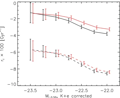
Figure 16.The change in average light luminosity per galaxy per Gyr, computed as per equation (30) as a function of faintest galaxy in the sample. The three panels show the different weighting schemes used when computing number and luminosity densities:Vmatchon the left, unweighted in the centre and

Vmaxon the right. The black line showsrg×100 for the full sample, and the red line for galaxies withg−i>2.35. When weighted byVmatch,rgshows

evidence for a slowly evolving population using both stellar population models (M11 in dashed lines, FSPS in the solid lines; we also show the purely passive model of Maraston et al. 2009 in the dotted red line – see Section 5.5.1 for details). The trend in the middle panel is dominated by incompleteness issues in the LRG sample, which are severe forMi0.55>−23 (see Figs 12 and 13).V/Vmaxweights (right) result in a lowrgdown to lower magnitudes thanV/Vmax,

but it rises steeply with decreasing luminosity beyond that. This could be a result of an inadequate completeness correction or increased merging rate at these luminosities. In any case, this comparison demonstrates clearly that the way in which theVmatchweights balance the two samples at low luminosities results

in a well-matched sample in terms of comoving densities and average luminosity per galaxy – as is our goal. Poisson errors are shown for one of the sets of models only for clarity – they are identical for the other set. See text for further discussion.

Here,r naturally tells a similar tale – for the same comoving

number density, LRGs hold less luminosity than CMASS galaxies. Removing galaxies with observed colourg−i<2.35 reduces this number by1 per cent at the faintest magnitudes, but a 5 per cent discrepancy remains, even for the reddest galaxies in the CMASS sample. As is obvious from the luminosity functions in Figs 12 and 13, these rates are heavily dependent on the slope of thek+ E

corrections. Results using the M11 models are identical in shape, but are lower by a factor of 2–3. That is, the uncertainty in the modelling of thek+Ecorrections can potentially overwhelm these statistics. We return to this at the end of this section. One point of interest is how theVmatch Mi0.55 CMASS luminosity function seems offset from that of the LRGs by an almost constant factor as a function of magnitude for both FSPS and M11 – this is likely a result of ak+Ecorrection slope that is too steep.

To help understand the observed evolution, we examine the rate of change in weighted luminosity per object, orrg as given by equation (30), which we show in the leftmost panel of Fig. 16. Recall that, for this statistic, we select galaxy samples based on a fixedk+Ecorrected absolute magnitude. Using either SPS model,

rgis between−1 (at the bright end) and 2 per cent (at the faint end). A steeper evolution seen with M11 is now clear, and it indicates that the typical luminosity per galaxy increases between the two surveys, especially at the faint end. A similar trend is seen using FSPS models, but it is less significant. Processes like merging would act to change the shape of the luminosity function, according to the fraction and magnitude of the merging galaxies. However, that is not what is observed in theMi0.55luminosity function witheither set of models. In other words, the fact that we observe a small value ofrgissupport for a slowly evolving weighted luminosity per

galaxybetween the two surveys. Note that the sign is positive – i.e.

[(n_LRG/_LRG)/(n_CMASS/_CMASS)] < 1, or in other words, there is on average more luminosity per galaxy in the LRG sample. This is now consistent with a small amount of luminosity growth through merging.

For comparison, we also showrgcomputed using unweighted number and luminosity densities, or usingVmax-corrected densi-ties. In the unweighted case, we see a much steeper trend in an inferred merger rate with luminosity. This trend is dominated by incompleteness issues within the LRG sample, which becomes se-rious at aroundMi0.55 = −23, as can be seen in the dashed lines of Figs 12 and 13. AV/Vmax weight results in a lower inferred merger rate down to lower magnitudes (Mi0.55= −22.5), but shows a steep trend of increasingrgwith decreasing luminosity beyond that. It is difficult to assess whether this effect is due toV/Vmaxbeing insufficient to fully correct for completeness or whether it is due to a steeper merging rate at those luminosities (which in turn are down-weighted using theVmatch approach). In any case, this com-parison demonstrates quite clearly that the way in which theVmatch weights balance the two samples at low luminosities results in a well-matched sample in terms of comoving densities and average luminosity per galaxy.

To summarize, we have a complicated scenario:rN andronly

reflect a true merger rate or luminosity growth in the absence of con-tamination or unresolved pairs, and a true concon-tamination/unresolved pairs fraction in the absence of merging. These two quantities are also sensitive to a change in the slope ofk+Ecorrections as they rely on matching samples by luminosity and number density. They show a significant excess of luminosity in CMASS, with respect to what we should expect from LRGs.rg, measuring the change in the average luminosity per object, is less sensitive both to the slope of thek+Ecorrection and to contaminants (provided they have

2012 The Authors, MNRAS424,136–156