Numerical analysis and multi precision computational methods applied to the extant problems of Asian option pricing and simulating stable distributions and unit root densities

NUMERICAL ANALYSIS AND MULTI-PRECISION

COMPUTATIONAL METHODS APPLIED TO THE

EXTANT PROBLEMS OF ASIAN OPTION PRICING AND

SIMULATING STABLE DISTRIBUTIONS AND UNIT

ROOT DENSITIES

L

iang Cao

A Thesis Submitted for the Degree of PhD

at the

University of St Andrews

2014

Full metadata for this item is available in

Research@StAndrews:FullText

at:

http://research-repository.st-andrews.ac.uk/

Please use this identifier to cite or link to this item:

http://hdl.handle.net/10023/6539

This item is protected by original copyright

Numerical Analysis and Multi-Precision

Computational Methods Applied to the Extant

Problems of Asian Option Pricing and Simulating

Stable Distributions and Unit Root Densities

Liang Cao

This thesis is submitted in partial fulfilment for the degree of

PhD Economics and Finance

at the

University of St Andrews

Numerical Analysis and Multi-Precision

Computational Methods Applied to the Extant

Problems of Asian Option Pricing and Simulating

Stable Distributions and Unit Root Densities

This thesis is submitted for the degree of

PhD Economics and Finance

Liang Cao

University of St Andrews

July 2014

Abstract

This thesis considers new methods that exploit recent developments in computer technology to address

three extant problems in the area of Finance and Econometrics. The problem of Asian option pricing has

endured for the last two decades in spite of many attempts to find a robust solution across all parameter

values. All recently proposed methods are shown to fail when computations are conducted using

standard machine precision because as more and more accuracy is forced upon the problem, round-off

error begins to propagate. Using recent methods from numerical analysis based on multi-precision

arithmetic, we show using the Mathematica platform that all extant methods have efficacy when

computations use sufficient arithmetic precision. This creates the proper framework to compare and

contrast the methods based on criteria such as computational speed for a given accuracy. Numerical

methods based on a deformation of the Bromwich contour in the Geman-Yor Laplace transform are

found to perform best provided the normalized strike price is above a given threshold; otherwise

This thesis considers new methods that exploit recent developments in computer technology to address

three extant problems in the area of Finance and Econometrics. The problem of Asian option pricing has

endured for the last two decades in spite of many attempts to find a robust solution across all parameter

values. All recently proposed methods are shown to fail when computations are conducted using

standard machine precision because as more and more accuracy is forced upon the problem, round-off

error begins to propagate. Using recent methods from numerical analysis based on multi-precision

arithmetic, we show using the Mathematica platform that all extant methods have efficacy when

computations use sufficient arithmetic precision. This creates the proper framework to compare and

contrast the methods based on criteria such as computational speed for a given accuracy. Numerical

methods based on a deformation of the Bromwich contour in the Geman-Yor Laplace transform are

found to perform best provided the normalized strike price is above a given threshold; otherwise

methods based on Euler approximation are preferred.

The same methods are applied in two other contexts: the simulation of stable distributions and the

computation of unit root densities in Econometrics. The stable densities are all nested in a general

function called a Fox H function. The same computational difficulties as above apply when using only

double-precision arithmetic but are again solved using higher arithmetic precision. We also consider

simulating the densities of infinitely divisible distributions associated with hyperbolic functions. Finally,

our methods are applied to unit root densities. Focusing on the two fundamental densities, we show our

methods perform favorably against the extant methods of Monte Carlo simulation, the Imhof algorithm

and some analytical expressions derived principally by Abadir. Using Mathematica, the main

1. Candidate’s declarations:

I, Liang Cao, hereby certify that this thesis, which is approximately 78000 words in length, has been written by me, that it is the record of work carried out by me and that it has not been submitted in any previous application for a higher degree.

I was admitted as a research student in March 2009 and as a candidate for the degree of PhD Economics and Finance in March 2010; the higher study for which this is a record was carried out in the University of St Andrews between 2009 and 2014.

Date signature of candidate

2. Supervisor’s declaration:

I hereby certify that the candidate has fulfilled the conditions of the Resolution and Regulations appropriate for the degree of PhD Economics and Finance in the University of St Andrews and that the candidate is qualified to submit this thesis in application for that degree.

Date signature of supervisor

3. Permission for electronic publication: (to be signed by both candidate and supervisor)

In submitting this thesis to the University of St Andrews I understand that I am giving permission for it to be made available for use in accordance with the regulations of the University Library for the time being in force, subject to any copyright vested in the work not being affected thereby. I also understand that the title and the abstract will be published, and that a copy of the work may be made and supplied to any bona fide library or research worker, that my thesis will be electronically accessible for personal or research use unless exempt by award of an embargo as requested below, and that the library has the right to migrate my thesis into new electronic forms as required to ensure continued access to the thesis. I have obtained any third-party copyright permissions that may be required in order to allow such access and migration, or have requested the appropriate embargo below.

The following is an agreed request by candidate and supervisor regarding the electronic publication of this thesis:

Add one of the following options:

(i) Access to printed copy and electronic publication of thesis through the University of St Andrews.

Date signature of candidate signature of supervisor

i

TABLE OF CONTENTS

Chapter 1: Introduction

... 1

1. Motivation ... 1

2. Overview ... 6

Chapter 2: Comparing New and Extant Numerical and Analytical Methods of

Asian Option Pricing

... 9

1. Introduction ... 9

1.1. Literature review ... 9

1.2. Motivation ... 13

2. Preliminary Material on Asian Options ... 15

2.1. The stock price ... 15

2.2. European options ... 15

2.3. Asian options ... 17

2.4. Pricing formulae for geometric Asian options ... 18

2.5. Black-Scholes equation ... 19

3. Numerical and Analytical Methods ... 21

3.1. Preliminaries ... 21

3.2. German and Yor's Laplace transform ... 25

3.3. Numerical inversion algorithms ... 30

3.4. Asymptotic method ... 46

3.5. PDE method ... 48

3.6. Spectral series expansion ... 52

ii

3.8. Turnbull and Wakeman's approximation ... 58

3.9. Milevsky and Posner's reciprocal gamma approximation ... 59

4. Numerical Results ... 61

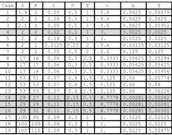
4.1. Experiment design ... 61

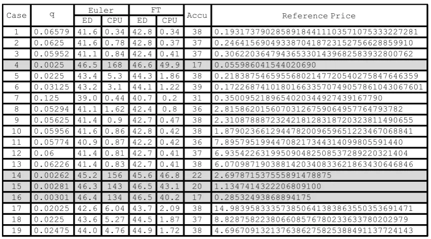
4.2. Reference prices of nineteen Asian option cases ... 63

4.3. Numerical results of the Euler method ... 64

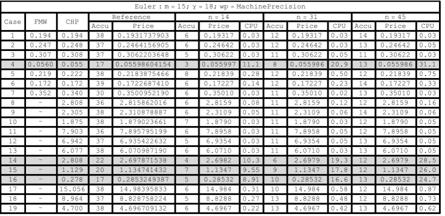
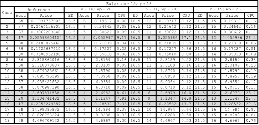
4.4. Numerical results of the Post-Widder method ... 66

4.5. Numerical results of Bromwich integration ... 68

4.6. Numerical results of the Gaver-Wynn-Rho algorithm ... 71

4.7. Numerical results for the fixed Talbot method ... 73

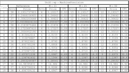
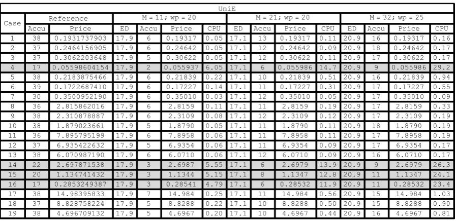
4.8. Numerical results of the unified Gaver-Stehfest algorithm ... 75

4.9. Numerical results of the unified Euler algorithm ... 77

4.10. Numerical results for the unified Talbot algorithm ... 79

4.11. Numerical results of the Laguerre method ... 81

4.12. Numerical results of the spectral series expansion ... 84

4.13. Numerical results of constructive complex analysis ... 86

4.14. Numerical results of TW, RG, PDE and asymptotic method ... 88

4.15. Numerical results of Monte Carlo simulation ... 89

5. Conclusion ... 91

Chapter 3: A Comparison of Various Methods for Computing Stable

Distributions and Infinitely Divisible Distributions Associated with Hyperbolic

Functions

... 93

1. Introduction ... 93

iii

2.1. Brownian motion ... 97

2.2. Brownian bridge... 98

2.3. Brownian meander and excursion ... 99

3. Infinitely Divisible Distributions Associated with Hyperbolic Functions ... 101

3.1. Definition of distributions ... 101

3.2. Properties of 𝐶𝐶

, 𝑆𝑆

and 𝑇𝑇

... 102

3.2. Laws of 𝐶𝐶̂

, 𝑆𝑆̂

and 𝑇𝑇�

... 107

4. Numerical Experiments with

𝐶𝐶

, 𝑆𝑆

and 𝑇𝑇

... 112

4.1. Computing the density of 𝐶𝐶

... 112

4.2. Computing the density of 𝑆𝑆

... 117

4.3. Computing the density of 𝑇𝑇

... 122

5. Stable Distributions ... 126

5.1. The Definition of 𝑆𝑆

(

𝛼𝛼

,

𝛽𝛽

,

𝜇𝜇

,

𝜎𝜎

)

... 126

5.2. The Definition of 𝑆𝑆

(

𝛼𝛼

,

𝛽𝛽

,

𝜇𝜇

,

𝜎𝜎

)

... 127

5.3. Generation of stable random variables 𝑆𝑆

(

𝛼𝛼

,

𝛽𝛽

)

... 129

5.4. Special functions related to stable distributions... 130

5.5. Densities of various stable distributions ... 131

6. Numerical Experiments with Stable Distributions ... 141

6.1. Computing the density 𝑔𝑔

... 141

6.2. Computing the density 𝑓𝑓

of generalized one-sided stable distribution 𝐹𝐹

142

6.3. Computing the density 𝑓𝑓

of one-sided stable distribution 𝐹𝐹

... 146

6.4. Computing the density 𝑓𝑓

of two-sided stable distribution 𝐹𝐹

... 150

7. Conclusion ... 153

iv

1. Introduction and Motivation ... 155

2. Unit Root Problem in AR(1) Model ... 160

2.1. Stationary case ... 160

2.2. Nonstationary case ... 161

2.3. Limiting distributions... 163

2.4. Test unit root hypothesis ... 165

3. Simulate the Distributions of

S

,

S

,

S

and

S

... 167

4. Computing the Distribution of

S

from the Characteristic Function... 172

4.1. Imhof's formula for 𝑆𝑆

... 172

4.2. Evaluating the characteristic function associated with 𝑆𝑆

... 173

4.3. Computing the distribution function of 𝑆𝑆

... 174

4.4. Computing the probability density of 𝑆𝑆

... 177

5. Joint Density of

U

and

V

... 185

5.1. The Laplace transform of the joint distribution

(

𝑈𝑈

,

𝑉𝑉

)

... 186

5.2. Computation of the density 𝑓𝑓

(

𝑣𝑣

)

... 187

5.3. Computation of the density 𝑓𝑓

(

𝑢𝑢

)

... 188

5.4. Computation of the joint density 𝑓𝑓

(

𝑢𝑢

,

𝑣𝑣

)

... 193

6. Joint Density of

R

and

S

... 199

6.1. Standardized quadratic forms ... 199

6.2. Formulae for joint density 𝑓𝑓

(

𝑟𝑟

,

𝑠𝑠

)

... 200

6.3. Formulae for joint distribution function 𝐹𝐹

(

𝑟𝑟

,

𝑠𝑠

)

... 204

7. Generating Densities of Unit Root Statistics ... 206

7.1. Transformation between 𝑓𝑓

(

𝑢𝑢

,

𝑣𝑣

)

and 𝑓𝑓

(

𝑟𝑟

,

𝑠𝑠

)

... 206

7.2. Generating the density of 𝑆𝑆

from 𝑓𝑓

(

𝑢𝑢

,

𝑣𝑣

)

... 208

v

7.4. Generating the density of 𝑆𝑆

from 𝑓𝑓

(

𝑢𝑢

,

𝑣𝑣

)

... 217

7.5. Generating the density of 𝑆𝑆

from 𝑓𝑓

(

𝑟𝑟

,

𝑠𝑠

)

... 222

8. Conclusion ... 227

Chapter 5: Conclusion

... 229

1. Contributions of the Thesis ... 229

1.1. Chapter 2 ... 229

1.2. Chapter 3 ... 230

1.3. Chapter 4 ... 231

1.4.

Mathematica

code ... 232

2. Suggestions for Further Work ... 233

Appendices ... 235

Bibliography ... 237

Mathematica

Code ... 241

1. Code in Chapter 2 ... 241

2. Code in Chapter 3 ... 286

Chapter 1

Introduction

1. Motivation

The Laplace transform is an integral transform which is widely used in finance and econometrics to, for

example, characterize the Asian option price, define probability distributions and represent the joint

density related to unit root distributions. This thesis seeks to apply state-of-the-art methods of Laplace

transform inversion and other numerical methods in an explicit multi-precision computing environment

to examine three problems that have endured in various fields: the problem of pricing an Asian option;

the problem of computing and simulating stable distributions and densities (we also consider other

infinitely divisible distributions associated with hyperbolic functions); and the problem of computing

and simulating unit root densities in Econometrics.

Let fHtL be a real-valued function of a real variable t>0. The Laplace transform of fHtL is defined as

(1.1)

f

` HsL=Ù

0 ¥

e-s t f HtLât

where s is a complex variable. It transforms the function fHtL in time domain to the function f`HsL in

complex domain by integration with the kernel e-s t.

Assume the above Laplace transform is well-defined and analytic for ReHsL>0. This ensures the region

of convergence of f

`

HsL covers the right half plane. This assumption is natural for a large class of

applications, but can be generalized for others by making a change of variables. Then, the inverse

Laplace transform also known as Bromwich integral is given by

(1.2)

fHtL= 1 2ΠiÙa-i¥

a+i¥

es t _f`H_sL_âs

where the integration is done along a vertical line s=a such that all singularities of f`HsL are to the left of

the contour path. This keeps the contour path in the region of convergence of f

` HsL.

where the integration is done along a vertical line s=a such that all singularities of f`HsL are to the left of

the contour path. This keeps the contour path in the region of convergence of f`HsL.

The Laplace transform can be applied in many areas. In finance, it is difficult to evaluate an Asian

option because the payoff of the Asian option depends on the average price of the underlying stock over

a prespecified period. The distribution of the average is too complicated to be characterized analytically.

Turnbull and Wakeman (1991) approximate the distribution of the average analytically by matching the

first two moments to the lognormal distribution, while Milevsky and Posner (1998) match them to the

reciprocal gamma distribution. The problem with analytical approximations is that there is no reliable

error estimates (Linetsky, 2004).

Geman and Yor (1993) have derived a closed-form expression for the Laplace transform of the

normalized Asian call price:

(1.3)

C` HΛ,qL=Ù₀¥e-ΛhCHΝLHh,qLâh= Ù0 1H2qL

e-x_xHΜ-ΝL2-2_{H1-2q xL}HΜ+ΝL2+1

âx

ΛHΛ-2-2ΝLGHHΜ-ΝL2-1L

where Μ = 2Λ + Ν2 and the normalized interest rate Ν, the normalized maturity h, and the normalized

strike price q are given by

(1.4)

Ν = 2Hr-∆L Σ2 -1

h= Σ

2

4 HT-tL

q= Σ

2

4SHtL9K T-Ù0

t

SHuLâu=

where r is the constant risk-free interest rate, ∆ is the constant dividend yield, Σ is the constant volatility,

K is the strike price, T is the time to maturity, and SHtL is the stock price at present time t. Ù₀tSHuLâu

divided by t stands for the realized average price over the time interval @0,tD. The process of numerically

inverting the Geman and Yor (1993) Laplace transform will lead to the normalized Asian call price from

which the Asian call price can be computed with ease. As we shall explain in Chapter 2, the Asian put

option price is related to the call price by the notion of “put-call parity”. Fu, Madan and Wang (1999)

and Craddock, Heath and Platen (2000) discuss and compare various inversion algorithms for the

problem of Asian option pricing. They show inversion of the Laplace transform encounters numerical

difficulties for low volatility and short maturity, and therefore do not recommend it as a method of

pricing an Asian option. But, they have not considered the factor of computation precision which

determines the round-off errors. Also, given that computers has now become much more powerful than a

where r is the constant risk-free interest rate, ∆ is the constant dividend yield, Σ is the constant volatility,

K is the strike price, T is the time to maturity, and SHtL is the stock price at present time t. Ù₀tSHuLâu

divided by t stands for the realized average price over the time interval @0,tD. The process of numerically

inverting the Geman and Yor (1993) Laplace transform will lead to the normalized Asian call price from

which the Asian call price can be computed with ease. As we shall explain in Chapter 2, the Asian put

option price is related to the call price by the notion of “put-call parity”. Fu, Madan and Wang (1999)

and Craddock, Heath and Platen (2000) discuss and compare various inversion algorithms for the

problem of Asian option pricing. They show inversion of the Laplace transform encounters numerical

difficulties for low volatility and short maturity, and therefore do not recommend it as a method of

pricing an Asian option. But, they have not considered the factor of computation precision which

determines the round-off errors. Also, given that computers has now become much more powerful than a

decade ago, the conclusion would be different.

The infinitely divisible distributions of non-negative random variables Ct, St and Tt can be characterized

by Laplace transforms (Pitman and Yor, 2003): for t ³0,

(1.5)

EAe-ΛCtE₌Ù

0 ¥

e-Λx fCtHxLâx=J

1

cosh 2Λ N

t

EAe-ΛStE₌Ù

0 ¥

e-Λx fStHxLâx=K

2Λ sinh 2Λ O

t

EAe-ΛTtE₌Ù

0 ¥

e-Λx fTtHxLâx=K

tanh 2Λ 2Λ O

t

The laws of Ct and St occur naturally in the study of Brownian motion and Bessel processes (Yor, 1997,

§18.6 cited in Pitman and Yor, 2003). The distribution of C12 arises when studying the Dickey-Fuller

distributions. Analytical formulae have been derived for the density of Ct for general t (Biane, Pitman

and Yor, 2001), the density of St for general t (Biane and Yor, 1987 cited in Biane, Pitman and Yor,

2001), the densities of C1 and S1 (Devroye, 2009a), and the density of S12 (Tolmatz, 2002). Note the

formula for the density of St is intractable other than t=1. Also, the formula for the density of Tt is not

available. If the Laplace transforms of Ct, St and Tt can be inverted numerically, the densities of Ct, St

and Tt for general t will be obtained.

The stable distributions are a class of distributions such that a linear combination of two i.i.d. stable

random variables has the same distribution up to location and scale parameters. There are many types of

stable distributions including SHΑ, Β,Μ,ΣL, S1HΑ, Β1,Μ,Σ1L, the generalized one-sided stable

distribution Fm,Α, the one-sided stable distribution FΑ and the two-sided stable distribution FΑ,Β. The first

two stable distributions can be conveniently described by their characteristic functions. While, Fm,Α, FΑ

and FΑ,Β discussed in the paper by Schneider (1987) are defined by some probability density gm,Α, the

Laplace transform and the Fourier transform respectively. Let fΑ be the density of FΑ. The Laplace

transform of fΑ is given by

(1.6) Ù0

¥

e-Λx _f

ΑHxLâx=e-Λ

Α

Let fm,Α be the density of Fm,Α. Schneider (1987) obtains the Laplace transform of fm,Α which can be

expressed in terms of the Fox function. In the special case of m=1, 2, the Laplace transform of fm,Α has

a closed-form expression.

Let fm,Α be the density of Fm,Α. Schneider (1987) obtains the Laplace transform of fm,Α which can be

expressed in terms of the Fox function. In the special case of m=1, 2, the Laplace transform of fm,Α has

a closed-form expression.

For m=1,

(1.7) Ù0

¥

e-Λx f1,ΑHxLâx=e -JΛ

bN

Α

where b=J Α

GH1-ΑLN 1Α

.

For m=2,

(1.8) Ù0

¥

e-Λx f2,ΑHxLâx= 2 GHΒLI

Λ

bM

12 KΒ 2I

Λ

bM 1

2Β

where Β = 1

1+Α and KnHzL is the modified Bessel function of the second kind.

The distribution SHΑ, Β,Μ,ΣL can be computed or simulated by Mathematica 9.0 built-in function

StableDistribution@ D. The distribution S1HΑ, Β1, 0, 1L can be simulated by a recipe proposed by

Chambers, Mallows and Stuck (1976). Schneider (1987) derives Fox function representations and series

expansions for the densities fm,Α, fΑ and fΑ,Β where fΑ,Β is the density of FΑ,Β. Alternative series

expansions for fΑ,Β can be found in the Feller’s (1970, p.583) text. Penson and Gorska (2011) show the

density fΑ for rational Α =lk can be written as a finite sum of generalized hypergeometric functions.

Schneider (1986) and Garoni and Frankel (2002) give special function representations for the special

cases of fΑ,Β, which correct f23,0 and recover f12,0 discussed by Zolotarev (1954). The density fΑ,Β can

also be computed by numerical inversion of the Fourier transform. By numerical inversion of the

associated Laplace transforms, we can obtain the densities fm,Α and fΑ. But, the complete relations

between SHΑ, Β,Μ,ΣL, S1HΑ, Β1,Μ,Σ1L, Fm,Α, FΑ and FΑ,Β has been lacking, and is therefore worth

studying.

When studying the first order autoregressive time series under a unit root, the so-called Dickey-Fuller

distributions of random variables S3 and S4 are of interest to many researchers. As the limiting cases of

unit root statistics S3T and S4T with the notation used in Tanaka (1996), S3 and S4 can be expressed in

(1.9)

S3=

U

V

S4=

U

V

with

(1.10)

U =Ù₀1wHtLâwHtL= 1 2Aw

2H₁L_-1E

V=Ù₀1w2H_tL_ât

where wHtL is a standard Brownian motion with t Î@0, 1D. The distributions of S3 and S4 were first

approximated by Monte Carlo simulation with finite samples (Fuller, 1976 cited in Tanaka, 1996, p.17),

but the approximations are usually poor especially on the tails. The distribution of S3 was computed

numerically from the associated characteristic function (Tanaka, 1996). However, the problem of

computing the Dickey-Fuller distributions properly remains unsolved. We notice that the densities of S3

and S4 can be constructed from the joint density fU,VHu,vL of HU,VL provided that the joint density is

readily available.

White (1958, p.1193) have derived the Laplace transform of HU,VL

(1.11)

fŽHΑ, ΒL=E@expH- ΑU- ΒVLD

=Ù₀¥Ù_-¥_12e-Αu- Βv fU,VHu,vLâuâv

=eΑ2 cosh 2Β + Α 2Β

sinh 2Β

-12

As we can see, the joint density fU,VHu,vL is embedded in the above Laplace transform which is

two-dimensional. Theoretically, numerical inversion of two-dimensional Laplace transforms will result in the

joint density fU,VHu,vL. But this needs to be verified by numerical experiments.

Nonetheless, numerical inversion of Laplace transforms is non-trivial. It involves a lot of effort, very

careful selection for inversion parameters, and specification for computation precision. In general, the

difficulty of the inversion mainly depends on the Laplace transform to be inverted and inversion

algorithm used. The inversion algorithms to be considered in this thesis include the Euler method (Euler)

and the Post-Widder method (PW) proposed by Abate and Whitt (1995); the Laguerre method

(Laguerre) suggested by Abate, Choudhury and Whitt (1996); the Bromwich integral (Bromwich)

applied by Shaw (1998); the fixed Talbot method (FT) and the Gaver-Wynn-Rho algorithm (GWR)

presented by Abate and Valkó (2004); and three inversion routines in the unified framework (Abate and

Whitt, 2006): the unified Gaver-Stehfest algorithm (UniG), the unified Euler algorithm (UniE), and the

unified Talbot algorithm (UniT). Among them, UniG, UniE and UniT can be combined to form nine

different two-dimensional inversion algorithms (Abate and Whitt, 2006): UniTG, UniTT, UniEG,

UniET, UniTE, UniGT, UniGG, UniEE and UniGE with first operator, say T, applying to the outer loop

and the second operator, say G, applying to the inner loop.

Nonetheless, numerical inversion of Laplace transforms is non-trivial. It involves a lot of effort, very

careful selection for inversion parameters, and specification for computation precision. In general, the

difficulty of the inversion mainly depends on the Laplace transform to be inverted and inversion

algorithm used. The inversion algorithms to be considered in this thesis include the Euler method (Euler)

and the Post-Widder method (PW) proposed by Abate and Whitt (1995); the Laguerre method

(Laguerre) suggested by Abate, Choudhury and Whitt (1996); the Bromwich integral (Bromwich)

applied by Shaw (1998); the fixed Talbot method (FT) and the Gaver-Wynn-Rho algorithm (GWR)

presented by Abate and Valkó (2004); and three inversion routines in the unified framework (Abate and

Whitt, 2006): the unified Gaver-Stehfest algorithm (UniG), the unified Euler algorithm (UniE), and the

unified Talbot algorithm (UniT). Among them, UniG, UniE and UniT can be combined to form nine

different two-dimensional inversion algorithms (Abate and Whitt, 2006): UniTG, UniTT, UniEG,

UniET, UniTE, UniGT, UniGG, UniEE and UniGE with first operator, say T, applying to the outer loop

and the second operator, say G, applying to the inner loop.

2. Overview

This thesis investigates a series of methods for numerically inverting Laplace transforms and applies

them to various problems. The inversion technique is also compared with other methods such as Monte

Carlo simulation, PDE method, analytical formulae and so on. We write Mathematica code for each

method. The numerical experiments are conducted in Mathematica 9.0 on a HP ProBook 4520s laptop

equipped with 2.4GHz Intel Core i3-370M processor and 3GB DDR3 RAM.

Chapter 2 deals with the problem of Asian option pricing. Inversion algorithms such as Euler, PW,

Laguerre, Bromwich, FT, GWR, UniG, UniE, and UniT are used to invert the Geman and Yor (1993)

Laplace transform. All computations are done with arbitrary-precision arithmetic rather than

machine-precision arithmetic where the latter is used by Fu, Madan and Wang (1999) and Craddock, Heath and

Platen (2000). Hence, the round-off errors can be controlled properly: round-off errors do not propagate

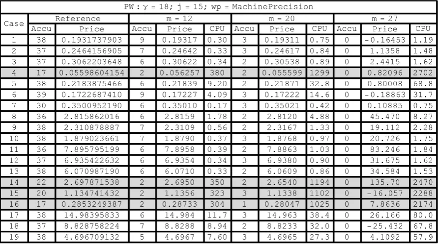
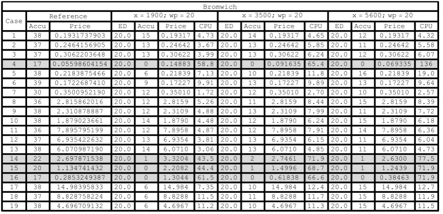
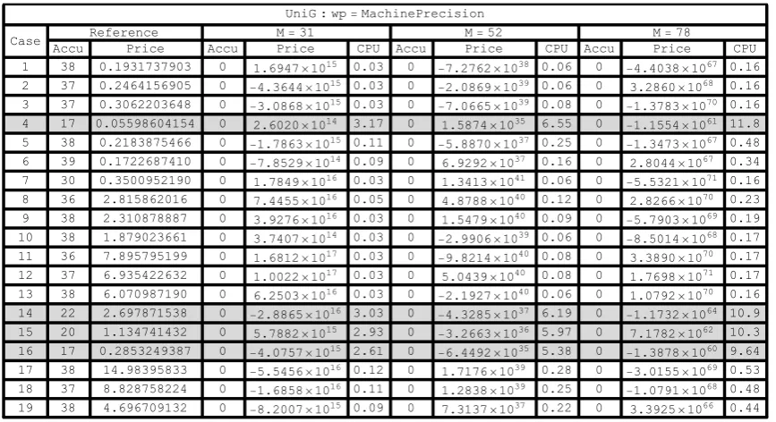
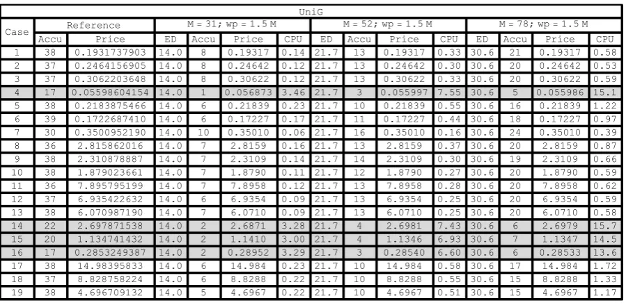
when one increases parameter values of the inversion algorithms. Eventually, by specifying appropriate

parameter values for each method we find all inversion algorithms achieve the same result. The matched

result can be computed to have high accuracy so that we can use it as the reference price to check the

accuracy of each method with its parameter settings. By manipulating the parameter settings for a

method, we can also see how the accuracy changes with different parameter values. It is found that the

truth of difficulties with numerical inversion for Asian option pricing is that the accuracy of the

algorithm drops and the computation time increases when the volatility is low and the maturity is short.

But we can regain the accuracy by increasing both the parameter values of the algorithm and the

computation precision at the cost of extra computation time.

In addition to numerical inversion, we consider many other methods for pricing an Asian option. These

methods include Monte Carlo simulation, analytical approximations (Turnbull and Wakeman, 1992;

Milevsky and Posner, 1998), PDE method (Rogers and Shi, 1995; Ve e , 2001; 2002), asymptotic

expansions (Shaw, 2002), spectral expansions (Linetsky, 2004) and constructive complex analysis

In addition to numerical inversion, we consider many other methods for pricing an Asian option. These

methods include Monte Carlo simulation, analytical approximations (Turnbull and Wakeman, 1992;

Milevsky and Posner, 1998), PDE method (Rogers and Shi, 1995; Ve e , 2001; 2002), asymptotic

expansions (Shaw, 2002), spectral expansions (Linetsky, 2004) and constructive complex analysis

(Schröder, 2008). With the reference prices, the accuracy of all methods can be verified.

Chapter 3 investigates various methods for computing infinitely divisible distributions and stable

distributions. Following Biane, Pitman and Yor (2001), we derive the formula for the density of St for

general t using Mathematica. The exact relations between different types of stable distributions are

established. Inversion algorithms UniG, UniE and UniT are applied to numerically inverting the Laplace

transforms associated with the infinitely divisible distributions and stable distributions with the yielded

results compared with those of analytical formulae. We show that UniG is a universal method for the

densities of St, Ct and Tt for general t>0, while UniE and UniT only work for the densities of St and Ct

for integer t >0 though they can compute the density of Tt for general t>0. When only the density of Tt

is concerned, UniE and UniT become superior to UniG in terms of the speed. With regard to the

computations of fm,Α and fΑ, UniE, UniT and UniG are all able to invert their Laplace transforms with

UniT faster than the other two.

Chapter 4 studies the unit root distributions S3 and S4 arising in AR(1) model with S3 =UV and

S4 =U‘ V , and seeks to compute the densities of S3 and S4 in a numerical way rather than based on

the approximations of Monte Carlo simulation. Following Tanaka (1996), we compute the density of S3

from the associated characteristic function using Imhof’s (1961 cited in Tanaka, 1996, p.196) formula.

However this method cannot be applied to the computation of the density of S4. Then, we attempt to

construct the densities of S3 and S4 from the joint density fU,VHu,vL. Given the original two-dimensional

Laplace transform of HU,VL, we reduce it to a one-dimensional Laplace transform of fU,VHu,vL with

respect to v. It is shown that the reduced Laplace transform can be inverted by UniG. With the numerical

results of fU,VHu,vL, we are able to generate not only the densities of S3 and S4 but also the density of

almost any unit root distribution which can be expressed in terms of U and V only. In addition, Abadir

(1995) proposes analytical formulae for the joint density fR,SHr,sL of HR,SL with R= 2 U and

S=2V. We establish a relation between fU,VHu,vL and fR,SHr,sL, and demonstrate fR,SHr,sL can also be

used for the generation of unit root distributions. By comparing results computed from fU,VHu,vL and

those computed from fR,SHr,sL, we find that using fU,VHu,vL is better than using fR,SHu,vL.

Chapter 4 studies the unit root distributions S3 and S4 arising in AR(1) model with S3 =UV and

S4 =U‘ V , and seeks to compute the densities of S3 and S4 in a numerical way rather than based on

the approximations of Monte Carlo simulation. Following Tanaka (1996), we compute the density of S3

from the associated characteristic function using Imhof’s (1961 cited in Tanaka, 1996, p.196) formula.

However this method cannot be applied to the computation of the density of S4. Then, we attempt to

construct the densities of S3 and S4 from the joint density fU,VHu,vL. Given the original two-dimensional

Laplace transform of HU,VL, we reduce it to a one-dimensional Laplace transform of fU,VHu,vL with

respect to v. It is shown that the reduced Laplace transform can be inverted by UniG. With the numerical

results of fU,VHu,vL, we are able to generate not only the densities of S3 and S4 but also the density of

almost any unit root distribution which can be expressed in terms of U and V only. In addition, Abadir

(1995) proposes analytical formulae for the joint density fR,SHr,sL of HR,SL with R= 2 U and

S=2V. We establish a relation between fU,VHu,vL and fR,SHr,sL, and demonstrate fR,SHr,sL can also be

used for the generation of unit root distributions. By comparing results computed from fU,VHu,vL and

those computed from fR,SHr,sL, we find that using fU,VHu,vL is better than using fR,SHu,vL.

Chapter 2

Comparing New and Extant

Numerical and Analytical Methods

of Asian Option Pricing

1. Introduction

Ÿ 1.1. Literature review

Asian options are financial derivatives whose payoffs are based on the average price of the underlying

asset over some prescribed period of time. Owing to the averaging feature, Asian options are widely

used in the stock market, the foreign exchange market and the commodity market. There are several

reasons why they are popular. First, the companies with sales in foreign currency are faced with the

unanticipated changes in the exchange rate between the foreign currency and the home currency. Asian

options provide them with an option of using the average foreign exchange rate to avoid the foreign

exchange risk. Second, it may be possible for large market participants to manipulate the prices in thinly

traded markets such as the crude oil market and the gold market. But it is much harder for them to

manipulate the average price with the existence of Asian options. Thirdly, Asian options are usually

cheaper than the ordinary options because the volatility of the average price is lower than the volatility of

the price itself.

Asian options receive their name Asian because they were first priced in Tokyo by David Spaughton and

Mark Standish of Bankers Trust who were there in 1987 on business developing ‘the first commercially

used pricing formula for options linked to the average of crude oil’ (Wilmott, 2006, p.427). There are

many types of Asian options depending on whether the option is a call or a put, where the average price

is used, what type the average is, and how to sample the underlying price over a time period. The

average price can be used either in place of the underlying price (an average price option) or in place of

the strike price (an average strike option). The average can be arithmetic or geometric. The sampling can

also be continuous or discrete. In this chapter, we mainly focus on the valuation of the continuously

sampled arithmetic average price call option (or continuous arithmetic Asian call in short) because it is

the case of greatest importance in terms of being type of Asian option that is traded most. It has also

been the type of Asian option most focused on in the academic literature.

Asian options receive their name Asian because they were first priced in Tokyo by David Spaughton and

Mark Standish of Bankers Trust who were there in 1987 on business developing ‘the first commercially

used pricing formula for options linked to the average of crude oil’ (Wilmott, 2006, p.427). There are

many types of Asian options depending on whether the option is a call or a put, where the average price

is used, what type the average is, and how to sample the underlying price over a time period. The

average price can be used either in place of the underlying price (an average price option) or in place of

the strike price (an average strike option). The average can be arithmetic or geometric. The sampling can

also be continuous or discrete. In this chapter, we mainly focus on the valuation of the continuously

sampled arithmetic average price call option (or continuous arithmetic Asian call in short) because it is

the case of greatest importance in terms of being type of Asian option that is traded most. It has also

been the type of Asian option most focused on in the academic literature.

The problem of pricing arithmetic Asian options has interested many researchers for more than two

decades as there are no closed-form formulae for them. The arithmetic average is not lognormally

distributed (McDonald, 2006, p.593) when the stock price follows geometric Brownian motion as in the

traditional framework in finance, the Black-Scholes framework, following from assumptions laid out by

Black and Scholes (1973). See, e.g. McDonald (2006, pp.649-650) or some other similar textbook. In

contrast to arithmetic average, the geometric average is lognormally distributed since the product of

lognormal random variables is also lognormal (McDonald, 2006, p.593). Therefore, closed-form

formulae exist for geometric Asian options.

The continuous arithmetic Asian call options were in the past valued using Monte Carlo simulation with

the control variate method, which is a variance reduction technique, by Kemna and Vorst (1990), where

they notice the continuous geometric Asian call serves as a quality control variate. Boyle, Broadie and

Glasserman (1997) further improve the equation for the control variate estimate of which the variance

can be minimized. Although Monte Carlo method is straightforward for path-dependent options such as

Asian options, it is often computationally expensive. Also, discretely sampling a continuous time process

results in the discretization bias (Broadie, Glasserman and Kou, 1999). Then, analytical approximations

are used in the valuation of Asian options. Turnbull and Wakeman (1991) approximate the distribution

of the arithmetic average by matching the first two moments to the lognormal distribution. Later,

Milevsky and Posner (1998) match them to the reciprocal gamma distribution. Analytical

approximations are fast but have no reliable error estimates (Linetsky, 2004).

An important contribution is made by Geman and Yor (1993) who derive a closed-form expression for

the Laplace transform of the continuous arithmetic Asian call price. The call price Ct,THKL can be

expressed as

An important contribution is made by Geman and Yor (1993) who derive a closed-form expression for

the Laplace transform of the continuous arithmetic Asian call price. The call price Ct,THKL can be

expressed as

(1.1)

Ct,THKL= e-rHT-tL

T I

4SHtL

Σ2 MCH

ΝLH_h,qL

with SHtL the stock price at time t, K the strike price, T the time to maturity, r the constant risk-free

interest rate, and Σ the constant volatility. The normalized interest rate Ν, the normalized maturity h, and

the normalized strike price q are given by

(1.2)

Ν = 2Hr-∆L Σ2 -1

h= Σ

2

4 HT-tL

q= Σ2

4SHtL9K T-Ù0

t

SHuLâu=

where ∆ is the constant dividend yield, and Ù₀tSHuLâu divided by t stands for the realized average price

over the time period @0,tD. The Laplace transform of the normalized Asian call price CHΝLHh,qL with

respect to h is given by

(1.3)

C`HΛ,qL=Ù₀¥e-ΛhCHΝLHh,qLâh

= Ù0 1H2qL

e-x_xHΜ-ΝL2-2_{H1-2q xL}HΜ+ΝL2+1

âx

ΛHΛ-2-2ΝLGHHΜ-ΝL2-1L

where Μ = 2Λ + Ν2 _.

The Geman-Yor Laplace transform C`HΛ,qL makes it possible to price Asian options by numerical

inversion of the Laplace transform. Geman and Eydeland (1995) first invert the Geman-Yor Laplace

transform using the fast Fourier transform (FFT). Shaw (1998, p.208) evaluates the Geman-Yor Laplace

transform in Mathematica revealing that C` HΛ,qL can be expressed in terms of the Kummer confluent

hypergeometric function as discussed below. He further exploits built-in Mathematica function

NIntegrate@ D and inverts C`HΛ,qL based on the Bromwich integral (which is the contour integral involved

in Laplace transform inversion as discussed below). Fu, Madan and Wang (1999) price Asian options

using the Euler method and the Post-Widder method, which are two inversion algorithms proposed by

Abate and Whitt (1995). They compare and contrast numerical inversion methods with Monte Carlo

simulation, and find that numerical inversion techniques encounter numerical difficulties for low

volatility and short maturity, or specifically for Σ2H_T-tL_{<0.01. Craddock, Heath and Platen (2000)}

investigate and compare different approaches to the numerical inversion of the Geman-Yor Laplace

transform, and draw a similar conclusion that numerical inversion methods can be extremely

time-consuming and unreliable when the normalized strike price q is small, i.e. q<0.03. There are a number

of important inversion algorithms in the numerical analysis literature that have not yet been applied to

Asian option pricing. These methods include the Laguerre method proposed by Abate, Choudhury and

Whitt (1996); the Gaver-Wynn-Rho algorithm and the fixed Talbot algorithm by Abate and Valkó

(2004); and the unified Gaver-Stehfest algorithm, the unified Euler algorithm, and the unified Talbot

algorithm by Abate and Whitt (2006). One of the contributions of this thesis is to apply these algorithms

to Asian option pricing. Given they are currently the most effective algorithms for Laplace transform

inversion, it is not surprising that we are able successfully to apply them to Asian option pricing,

yielding computational methods that are competitive with, and sometimes supersede, the currently best

extant methods in the literature.

The Geman-Yor Laplace transform C`HΛ,qL makes it possible to price Asian options by numerical

inversion of the Laplace transform. Geman and Eydeland (1995) first invert the Geman-Yor Laplace

transform using the fast Fourier transform (FFT). Shaw (1998, p.208) evaluates the Geman-Yor Laplace

transform in Mathematica revealing that C` HΛ,qL can be expressed in terms of the Kummer confluent

hypergeometric function as discussed below. He further exploits built-in Mathematica function

NIntegrate@ D and inverts C`HΛ,qL based on the Bromwich integral (which is the contour integral involved

in Laplace transform inversion as discussed below). Fu, Madan and Wang (1999) price Asian options

using the Euler method and the Post-Widder method, which are two inversion algorithms proposed by

Abate and Whitt (1995). They compare and contrast numerical inversion methods with Monte Carlo

simulation, and find that numerical inversion techniques encounter numerical difficulties for low

volatility and short maturity, or specifically for Σ2H_T-tL_{<0.01. Craddock, Heath and Platen (2000)}

investigate and compare different approaches to the numerical inversion of the Geman-Yor Laplace

transform, and draw a similar conclusion that numerical inversion methods can be extremely

time-consuming and unreliable when the normalized strike price q is small, i.e. q<0.03. There are a number

of important inversion algorithms in the numerical analysis literature that have not yet been applied to

Asian option pricing. These methods include the Laguerre method proposed by Abate, Choudhury and

Whitt (1996); the Gaver-Wynn-Rho algorithm and the fixed Talbot algorithm by Abate and Valkó

(2004); and the unified Gaver-Stehfest algorithm, the unified Euler algorithm, and the unified Talbot

algorithm by Abate and Whitt (2006). One of the contributions of this thesis is to apply these algorithms

to Asian option pricing. Given they are currently the most effective algorithms for Laplace transform

inversion, it is not surprising that we are able successfully to apply them to Asian option pricing,

yielding computational methods that are competitive with, and sometimes supersede, the currently best

extant methods in the literature.

The value of the continuous arithmetic Asian option can be characterized by a partial differential

equation (PDE) (see Wilmott, 2006, p.431). Hence, the price of an Asian option can be found by solving

the partial differential equation. Rogers and Shi (1995) derive a one-dimensional PDE for both fixed and

floating strike Asian options, but this PDE is difficult to solve numerically (Ve e , 2002). Ve e (2001;

2002) provides an alternative one-dimensional PDE for both continuous and discrete arithmetic Asian

options. Ve e claims that his PDE can be easily implemented to give very fast and accurate results.

Other methods include asymptotic method for low volatility proposed by Shaw (2002), spectral

expansion by Linetsky (2004), and constructive complex analysis by Schröder (2008). Among them,

Shaw (2002) approximates the Mellin transform of the Laplace transform by exploiting an asymptotic

expansion of the quotient of Gamma functions. Linetsky (2004) attacks the pricing problem directly by

using an identity in law between the integral of geometric Brownian motion and the state of a

one-dimensional diffusion process, and developing spectral expansion for the Asian put price. The Asian call

price can be recovered by using the put-call parity. Schröder (2008) develops a two-stage approach to the

valuation of Asian options which first expresses the normalized Asian call price as a single contour

integral in terms of Hermite functions, and then represents the integral by series and asymptotic

expansions with error estimates.

Other methods include asymptotic method for low volatility proposed by Shaw (2002), spectral

expansion by Linetsky (2004), and constructive complex analysis by Schröder (2008). Among them,

Shaw (2002) approximates the Mellin transform of the Laplace transform by exploiting an asymptotic

expansion of the quotient of Gamma functions. Linetsky (2004) attacks the pricing problem directly by

using an identity in law between the integral of geometric Brownian motion and the state of a

one-dimensional diffusion process, and developing spectral expansion for the Asian put price. The Asian call

price can be recovered by using the put-call parity. Schröder (2008) develops a two-stage approach to the

valuation of Asian options which first expresses the normalized Asian call price as a single contour

integral in terms of Hermite functions, and then represents the integral by series and asymptotic

expansions with error estimates.

Ÿ 1.2. Motivation

The papers by Fu, Madan and Wang (1999) and Craddock, Heath and Platen (2000) are of central

importance in the literature because they have become seen as the benchmark in terms of an

experimental design that any method of Asian option pricing can be evaluated against. That said, their

own experiments were conducted in a fixed machine-precision computing environment and, as we shall

see, this can be severely limiting. As we demonstrate below, this is because there comes a point where

the round-off errors in calculations begin to propagate when more and more accuracy is forced upon the

pricing problem. Another two types of errors which are not properly handled are truncation errors and

discretization errors. The truncation errors occur when an infinite series is truncated, while the

discretization errors arise when an integral is approximated by the trapezoidal rule. A fact which both

papers fail to notice is that the round-off errors may rise correspondingly in the machine-precision

computing environment when one tries to increase algorithm parameters to reduce truncation errors and

discretization errors. In other words, the accuracy of the results is improved consistently with the

truncation size only when the round-off errors and the discretization errors are controlled.

Regarding the computation time, Fu, Madan and Wang (1999) and Craddock, Heath and Platen (2000)

conclude that numerical inversion of the Geman-Yor Laplace transform is unreliable and

time-consuming, especially for low volatilities and short maturities. This is true when machine-precision

arithmetic is used and the computations are done with outdated computing software and a fifteen-year

old computer. But, the results may be different when we use the more powerful CPU and the ultimate

application for computations, Mathematica.

This chapter draws a comparison of various numerical and analytical methods for Asian option pricing.

These methods include numerical inversion, the PDE method by Ve e (2002), asymptotic method by

Shaw (2002), spectral expansion by Linetsky (2004), constructive complex analysis by Schröder (2008),

the Turnbull and Wakeman (1991) approximation, the Milevsky and Posner (1998) approximation, and

Monte Carlo simulation. The algorithms considered for numerical inversion cover the Euler method, the

Post-Widder method, Bromwich integration, the Gaver-Wynn-Rho algorithm, the fixed Talbot

algorithm, the unified Gaver-Stehfest algorithm, the unified Euler algorithm, the unified Talbot

algorithm, and the Laguerre method. We use Mathematica 9.0 to perform numerical experiments, and

write Mathematica codes for these methods (with the exception of asymptotic method). All

computations are done with arbitrary-precision arithmetic on a laptop equipped with 2.4GHz Intel Core

i3-370M processor and 3GB DDR3 RAM.

This chapter draws a comparison of various numerical and analytical methods for Asian option pricing.

These methods include numerical inversion, the PDE method by Ve e (2002), asymptotic method by

Shaw (2002), spectral expansion by Linetsky (2004), constructive complex analysis by Schröder (2008),

the Turnbull and Wakeman (1991) approximation, the Milevsky and Posner (1998) approximation, and

Monte Carlo simulation. The algorithms considered for numerical inversion cover the Euler method, the

Post-Widder method, Bromwich integration, the Gaver-Wynn-Rho algorithm, the fixed Talbot

algorithm, the unified Gaver-Stehfest algorithm, the unified Euler algorithm, the unified Talbot

algorithm, and the Laguerre method. We use Mathematica 9.0 to perform numerical experiments, and

write Mathematica codes for these methods (with the exception of asymptotic method). All

computations are done with arbitrary-precision arithmetic on a laptop equipped with 2.4GHz Intel Core

i3-370M processor and 3GB DDR3 RAM.

The rest of this chapter is organized as follows. Section 2 defines Asian options in more detail and states

the basic problem of Asian option pricing we consider (in the Black-Scholes framework). Section 3

considers various approaches to Asian option pricing both methods that already exist in the literature and

new methods we propose that apply recent state-of-the-art work relevant to our problem. In Sections 2

and 3, there are many methods to consider and so, by necessity, these sections are long. But they have to

be if we want our treatment to be taxonomic and encompassing. One contribution of this thesis is in

collecting and in some cases recognizing, and then organizing in one place, relevant methods for Asian

option pricing from the Finance and Computational Statistics literature. A second contribution is to

provide dedicated Mathematica code to implement each and every method that is discussed. The first

key conclusion is that in a fixed machine-precision environment, all methods have their drawbacks in

some regions of the parameter space. This result is widely known (and indeed this is the reason why the

Asian option pricing problem has been so enduring) but here we provide the reason why this is so.

Turning the problem on its head, we then show in a multi-precision environment, where the computing

precision is allowed to vary in accordance with the method in hand, that all methods have efficacy

provided the computing precision is large enough. This is our second key conclusion. Comparing and

contrasting the various methods then becomes, properly, an exercise in assessing them on other criteria,

such as the speed of computation to achieve a given accuracy. Some results are reported in Section 4.

Section 5 concludes.

2. Preliminary Material on Asian Options

Ÿ 2.1. The Stock price

In the Black-Scholes option-pricing model, the stock price is assumed to follow the geometric Brownian

motion (Black and Scholes, 1973 cited in McDonald, 2006, pp.649)

(2.1)

âSHtL

SHtL = Α ât+ Σ âWHtL

where SHtL is the stock price, âSHtL the instantaneous change in the stock price, Α the expected return on

the stock, Σ the volatility of the stock, and WHtL the value of a Brownian motion at time t.

Brownian motion is a continuous stochastic process which has the following properties (McDonald,

2006, p.650):

è WH0L=0. Brownian motion always starts at the origin.

è WHt+sL-WHtL is normally distributed with mean zero and variance s. Mathematically,

WHt+sL-WHtL~ s NH0, 1L where NH0, 1L is a standard normal distribution.

è WHt+s1L-WHtL and WHtL-WHt-s1L are independently distributed for s1,s2>0. è WHtL is continuous everywhere.

Brownian motion WHtL is a martingale which means E@WHt+sL WHtLD=WHtL. The process WHtL is also

called a diffusion process.

In the risk-neutral pricing, (2.1) is written as (see McDonald, 2006, p.661):

(2.2)

âSHtL

SHtL =rât+ Σ âW

Ž HtL

where r is the risk-free interest rate, and WŽHtL is another Brownian motion. If the stock pays dividends at

the continuous rate ∆, we should replace r with r- ∆.

The geometric Brownian motion is a stochastic differential equation (SDE). The solution to it is given by

(see McDonald, 2006, p.596)

(2.3)

St =S0eJ

r-∆-1

2Σ

2_Nt+ΣWHtL

=S0eJ

r-∆-1

2Σ

2_{Nt+Σ t Z}

where Z is a standard normal random variable, i.e. Z~NH0, 1L. Equation (2.3) implies the stock price

follows a lognormal distribution.

Ÿ 2.2. European options

European options can only be exercised at expiration. There are two types of European options: call

options and put options. A call option gives the buyer the right but not the obligation to buy the

underlying stock for the strike price. While, a put option gives the owner the right but not the obligation

to sell the underlying stock for the strike price.

European options can only be exercised at expiration. There are two types of European options: call

options and put options. A call option gives the buyer the right but not the obligation to buy the

underlying stock for the strike price. While, a put option gives the owner the right but not the obligation

to sell the underlying stock for the strike price.

Let SHtL be the stock price at time t, K be the strike price, and T be the time to maturity. The payoff of a

call option is

(2.4) Call payoff =HSHTL-K, 0L+

where Hx, 0L+ denotes the maximum of 0 and x.

The payoff of a put option is

(2.5) Put payoff =@K-SHTL, 0D+

Then, the price of the option can be obtained by discounting the payoff of the option to the current time.

The famous Black-Scholes formula is derived by Black and Scholes (1973) and Merton (1973) for

pricing European options. McDonald (2006, Ch.12) shows the Black-Scholes formula is a limiting case

of the binomial formula for the price of a European option. The price of a European call option on a

stock is given by the Black-Scholes formula

(2.6)

CHS,K,Σ,r,T,∆L=S e-∆T_NH_d

1L-K e-r TNHd2L

where

(2.7)

d1 =

lnHSKL+Jr-∆+1

2Σ

2_NT

Σ T

d2 =d1- Σ T

The Black-Scholes formula has six input parameters: S the current price of the stock, K the strike price

of the option, r the continuously compounded risk-free interest rate, ∆ the continuously compounded

dividend yield on the stock, Σ the volatility of the stock, and T the time to maturity of the option. NHxL is

the cumulative normal distribution function of the standard normal distribution.

The Black-Scholes formula for a European put option is

(2.8)

PHS,K,Σ,r,T,∆L =K e-r TNH-d2L-S e-∆TNH-d1L

where d1 and d2 are the same as those in the Black-Scholes formula for a European call option.

The Black-Scholes call price is related to the Black-Scholes put price by the put-call parity (see

McDonald, 2006, p.378)

The Black-Scholes call price is related to the Black-Scholes put price by the put-call parity (see

McDonald, 2006, p.378)

(2.9)

PHS,K,Σ,r,T,∆L=CHS,K,Σ,r,T,∆L+K e-r T_{-S e}-∆T

Ÿ 2.3. Asian options

An Asian option is a path-dependent option of which the payoff depends on the average price of the

underlying asset over some period of time. There are many types of Asian options depending on whether

the option is a call or a put, whether the average is arithmetic or geometric, whether the average is

continuously sampled or discretely sampled, and whether the average is used in place of the stock price

or the strike price.

Assume the stock price St is evenly sampled N+1 times over the time interval @0,TD. The time period is

then h=TN. McDonald (2006, p.446) defines the discretely sampled arithmetic average as

(2.10)

A_dHTL= 1

N+1Úi=0

N _S

i h

and the discretely sampled geometric average as

(2.11)

GdHTL=HS0´Sh´ × × × ´SN hL 1

N+1

Suppose SHtL is the stock price at time t. If the average is continuously sampled, Wilmott (2006, p.431)

shows the continuously sampled arithmetic average over the period @0,tD is

(2.12)

AcHtL=

1

t Ù0

t

SHΤLâ Τ

and continuously sampled geometric average over the period @0,tD is

(2.13)

GcHtL=expI

1

t Ù0

t

logSHΤLâ ΤM

The arithmetic average is commonly used in practice. Since the sum of lognormal variables is not

lognormally distributed given that the stock price follows a lognormal distribution, options based on the

arithmetic average have no closed-form solutions. Although the geometric average is less common in

derivatives markets, it has computational convenience. There are closed-form formulae for options based

on the geometric average.

When the average is used in place of the stock price, the option is called average price option. When the

average is used in place of the strike price, the option is called average strike option. Let AHTL be the

arithmetic average, GHTL the geometric average, ST the stock price at maturity, and K the strike price.

Here are eight basic types of Asian option