Seeing the wood for the trees : philosophical aspects of classical, Bayesian and likelihood approaches in statistical inference and some implications for phylogenetic analysis

(1)

Full metadata for this item is available in Research@StAndrews:FullText at: http://research-repository.st-andrews.ac.uk/

Seeing the wood for the trees: philosophical aspects of classical, Bayesian and likelihood approaches in statistical inference and some implications for

phylogenetic analysis

Daniel Barker

Date of deposit 21 07 2014

Version This is an author version of this work.

Access rights © This item is protected by original copyright.

This work is made available online in accordance with publisher policies. This is an author version of this work which may vary slightly from the published version. To see the final definitive version of this paper please visit the publisher’s website. Citation for

published version

Barker, D. (2014). Seeing the wood for the trees: philosophical aspects of classical, Bayesian and likelihood approaches in statistical inference and some implications for phylogenetic analysis. Biology & Philosophy. doi:10.1007/s10539-014-9455-x Link to published

version

(2)

Seeing the wood for the trees: philosophical aspects of classical,

Bayesian and likelihood approaches in statistical inference and some

implications for phylogenetic analysis

Daniel Barker

Sir Harold Mitchell Building, School of Biology, University of St Andrews, St Andrews, Fife,

KY16 9TH, UK

(3)

Abstract

The three main approaches in statistical inference – classical statistics, Bayesian and likelihood –

are in current use in phylogeny research. The three approaches are discussed and compared, with

particular emphasis on theoretical properties illustrated by simple thought-experiments. The

methods are problematic on axiomatic grounds (classical statistics), extra-mathematical grounds

relating to the use of a prior (Bayesian inference) or practical grounds (likelihood). This essay aims

to increase understanding of these limits among those with an interest in phylogeny.

Keywords

Phylogeny

Statistics

Bayesian inference

Classical statistics

Likelihood

(4)

Introduction

Too often, debates as to the relative merits of maximum likelihood and Bayesian phylogeny

reconstruction are held in isolation from the theory and application of likelihood and Bayesian

statistics in general, or indeed of statistical inference in general, ‘the process whereby data are

observed and then statements are made about unknown features of the system that gave rise to the

data’ (Beaumont and Rannala 2004). When considering philosophical matters of statistical

inference, it is more natural to begin with the fundamental principles involved and also their

implications for simple case studies. Later, one might progress to consider the implications for

complicated case studies, such as phylogeny reconstruction.

First, I would like to set the scene, by a review of why we require statistics, the meaning of

probability and of the three main schools of statistics in current use: Bayesian, classical and

likelihood. Each school has strong justifications and is widely used in phylogenetic research, as well

as other areas of biology. Startlingly, each is fundamentally incompatible with the others. They

cannot be reconciled because they are seeking answers to different questions. From a likelihood

point of view, which currently happens to be my own point of view, the Bayesian approach asks a

question that is mathematically valid, though whose value is limited by extra-mathematical

considerations; and classical statistics is axiomatically invalid.

Partly because some results are similar or identical for the different approaches, and partly because

practitioners tend to jump in to a complex case-study without devoting attention to the basics, these

fault lines often go unnoticed, are masked by more pressing difficulties with the input data (e.g.

(5)

A separate approach to the question is to compare methods as implemented in practice by software,

as opposed to the more theoretical approach taken here (e.g. Douady et al. 2003; Guindon and

Gascuel 2003; Yang and Rannala 2005; Simmons and Norton 2013). Such an approach is extremely

valuable to highlight the difference in inferences made by different methods. Where the data are

simulated, the disparity between the true phylogeny and the reconstructed phylogeny may also be

assessed. However, conclusions from practical analyses are dependent on the specific data analysed,

including (for simulations) the models used to simulate those data. Theoretical considerations are

also valuable, contributing to understanding by a different route, relevant even to conditions which

have not yet been thought of. The current paper emphasises theoretical considerations, particularly

in the first part which is most general, whilst also linking to the extensive literature on practical

properties, particularly in the latter part which is more closely tied to the problem of phylogeny

reconstruction.

Statistics

When we run an experiment (intended in a broad sense, including everything that is required to

reconstruct phylogeny), from the data we want to know: what is the truth here? Is this coin fair or

not? Is there a monophyletic clade Ecdysozoa or not? At which date did cyanobacteria originate?

These are the kinds of absolute knowledge we crave.

Such answers are wholly unavailable. What we get with statistics is a quantitative answer to a very

specific question. We will never know the truth exactly. Instead, statistics will provide us with some

quantitative indication of the probability of hypotheses (Bayesian statistics), the evidence against

(6)

are supported (likelihood). These answers are simultaneously deeply disappointing, because they do

not reveal truth as such, and almost miraculous, in that they pull some kind of indication of the truth

out of a mass of data which may be literally incomprehensible otherwise. A further source of

disappointment and/or wonder is that these partial answers, from the three main schools of statistics,

by definition can fail to coincide.

Statistics is a young field. As Kahneman (2012, 179) says, regression is such a difficult concept it

was not invented until 200 years after the theory of gravitation. (Statistics is not rocket science – but

rather, something a little more involved.) And this was 130 years ago – after Lamarck and Darwin,

contemporary with D’Arcy Thompson and Wallace – the time of our great grandparents, not some

mind-blowingly remote intellectual stone-age.

Probability

Statistical analyses all depend upon a concept of probability. Although there is agreement on the

axioms relating to probability, such as its sum rule and product rule, there is no general agreement

on the meaning of probability itself.

The Bayesian view of probability is that it indicates degree of belief, ranging from total disbelief (a

probability of 0) to total belief (a probability of 1), though there is a question as to whether the

upper and lower limits are ever really reached (Kadane 2011, 6). The Bayesian view of probability

is essential to Bayesian inference, but is in conflict with the view of probability required for

(7)

The frequentist view of probability is that probability indicates frequency in the long run, ranging

from something that never occurs (a probability of 0) to something that always happens (a

probability of 1). The frequentist view of probability is essential to classical and likelihood

inference, but is in conflict with Bayesian inference in general.

Bayesian inference

Bayesian inference is the oldest of the three statistical methods considered in this paper. One

approaches the data with a well-defined prior probability distribution, typically not based on the

evidence at hand; this is then updated on the basis of the evidence at hand, giving a posterior

probability for hypotheses. This allows one to quantify belief in hypotheses. Change either the data

at hand or the prior belief, and the posterior probability also changes.

Where the prior is known or else is ‘learnt’ from relevant training data, Bayesian approaches are

uncontroversial. In such cases, the prior probability is equally acceptable whether regarded as belief

or as frequency in the long run. For making predictions based on features learnt from data (i.e.

empirical priors), no-one objects to a Bayesian approach (e.g. Edwards 1977), though as in any

analysis the details are open to discussion. In prediction, we ‘do the best we can’ and divergence

from fact can be assessed by reference to known data, in a way that is not possible for complex

problems of inference. Bayesian approaches such as penalised likelihood and the lasso (Firth 1993;

Tibshirani 1996; Bühlmann and van de Geer 2011) have achieved enormous success in fields of

prediction, including bioinformatics (e.g. Lim et al. 2013; Lv et al. 2013). A vast range of methods

of sequence analysis incorporate Bayesian techniques (Durbin et al. 1998; Baldi and Brunak 2001;

(8)

For problems of statistical inference, in general there is no prior based on empirical evidence.

Empirical Bayes (Casella 1985; Efron 2003) is a useful development, in which the prior is obtained

via the data and model at hand. This is relatively uncontroversial and has important phylogenetic

applications, for example in detecting positive selection and in ancestral state reconstruction (Yang

et al. 1995; Nielsen and Yang 1998; Pagel 1999). Perhaps because of the complexity of the

inference problem, empirical Bayes in the central task of phylogeny reconstruction is relatively

underdeveloped (but cf. Yang and Rannala 2005). Instead, a ‘fully Bayesian’ (hierarchical Bayesian)

approach is used, with a subjective prior not based on the data at hand. This prior is based, for

example, on literature precedent, or very often just on software defaults. This is the controversial

aspect of Bayesian inference.

Classical inference

I use ‘classical’ to refer to any statistical test which relies on consideration of experiments that were

not actually performed. This includes p-values, confidence intervals and randomisation tests such as

the bootstrap. Classical statistics is often referred to as frequentist, which is true but is confusing

because the frequentist view of probability is also used elsewhere (likelihood).

In classical statistics, one approaches the data with a view as to how those data were obtained;

intervals, based on areas under a probability density function, may then be calculated. For example,

the p-value is the probability of observing a statistic with a value at least as extreme as the value

(9)

probability of hypotheses themselves, hence a Bayesian would argue these methods are answering

the wrong question.

Practical classical statistics, including p-values and confidence intervals, is very widely taught to

undergraduates. Yet p-values and confidence intervals remain almost equally widely misunderstood.

Students, and even worse instructors, often replace the correct definition with something incorrect

but more intuitive. For example, often one finds student answers along the lines that ‘a low p-value

indicates the null hypothesis is improbable’. Certainly a lower p-value indicates lower probability

for the null hypothesis than does a higher p-value. But this cannot be quantified because the p-value

is conditional on the null hypothesis being true. Hence, a p-value of 0.04 indicates the null

hypothesis is less probable than does a p-value of 0.05; but a p-value of 0.05 does not indicate the

probability of the null hypothesis is 0.05, or any other particular value (e.g. Lindley 1957). Moving

from a p-value to a statement about the probability of the null hypothesis requires some prior view

on the relative plausibility of the null and alternative hypotheses – a view which is not incorporated

into the classical statistical framework.

Another major tool in classical statistics is the confidence interval. The correct definition of

confidence intervals is so convoluted as to be only rarely understood (and will not be repeated here,

since p-values will be our main example for classical statistical inference). Instead the definition of

confidence intervals is often intuitively replaced by a different definition that really corresponds to a

‘fiducial interval’, although these two types of interval do not generally coincide (Fisher 1956,

(10)

These problems may hint at the possibility that classical statistics is answering the wrong questions,

or to put more positive spin on it, answering the right questions in the wrong way; or that classical

statistics is deceptively more difficult than it may appear, and almost everyone is innately bad at it.

Likelihood inference

Likelihood inference rejects the Bayesian use of priors and rejects classical statistics as

axiomatically invalid. For a given set of observations, the likelihood of a hypothesis is a relative

measure of how frequently the data would be observed, if that hypothesis were true. For a given set

of observed data, ratios between likelihoods for different hypotheses indicate their relative support.

The maximum likelihood hypothesis is the hypothesis which would lead to the data actually

observed, more often than any other hypothesis.

Likelihood inference is subtly but crucially different from classical inference, which when

interpreting evidence considers statistics more extreme than the value actually observed (in the case

of a p-value) or experiments which were not performed (in the case of confidence intervals).

Likelihood inference rejects, as irrelevant, these non-observed results from non-performed

experiments. But in common with classical statistics and in contrast to Bayesian statistics, it regards

(11)

Foundations of likelihood inference

One justification for likelihood inference is that it fulfils the criteria one would hope for in a system

of inference, in which case it is accepted as axiomatically correct (Edwards 1992, 28-31; Royall

2000). For given observed data and probability model, the relative support for different hypotheses

is expressed only by ratios of points on the likelihood function,

L(H|D) = k.P(D|H), (1)

where L(H|D) is the likelihood of a hypothesis H for the observed data D, P(D|H) is the probability

of the data D if H were true, and k is an arbitrary constant. If the likelihood axiom is acceptable to a

research worker, no further foundation is required.

In Bayesian statistics, the likelihood axiom is accepted, for the part of the inference based on the

evidence at hand, automatically due to Bayes’ theorem. One may write Bayes’ theorem as

P(H|D) = k.P(H).L(H|D), (2)

where P(H|D) is the posterior probability of hypothesis H for observed data D, P(H) is the prior

probability of the hypothesis and k ensures the posterior distribution integrates to 1 (e.g. Edwards

1992, 48). This highlights the two bases of Bayesian inference: the prior probability P(H), which

does not usually depend on on the data at hand; and the likelihood function L(H|D), which does.

Where one is uncomfortable with the use of priors in Bayesian inference, and not ready to

(12)

basis for likelihood inference. The likelihood principle (axiom) has been shown to follow from two

other, widely acceptable axioms: the principle of sufficiency and the principle of conditionality

(Birnbaum 1962). Only likelihood inference, and the aspect of Bayesian inference relating to the

data at hand, are compatible with both of these axioms simultaneously (Birnbaum 1962; Berger and

Wolpert, 1984; Gandenberger 2014). The likelihood principle may also be arrived at by other means

(e.g. Birnbaum 1972; Gandenberger 2014) but remains incompatible with classical statistics (Mayo

2010; Gandenberger 2014).

Case study: sufficiency in a coin-tossing experiment

Imagine two independent scientists are observing a coin-tossing robot, to obtain data to estimate the

probability of heads for a given coin. One scientist decides in advance to stop making observations

after four coin tosses, whatever the number of heads and tails. The other decides in advance to stop

making observations after seeing three heads, however many tosses this requires. The two scientists

start their observations at the same time. They observe the sequence: heads, heads, tails, heads. Both

go home to analyse the data. Should their different stopping rules affect their inferences?

Classical statistics says ‘yes’. For hypotheses about the probability of heads (or of tails), the first

scientist’s stopping rule suggests a binomial null distribution; the second suggests a negative

binomial null distribution. The estimate of the probability of heads is the same in each case (3/4),

but the different distributions give different p-values for hypothesis tests concerning this estimate.

By the principle of sufficiency in likelihood inference and also as a consequence of Bayes’ theorem

(13)

probability of heads, for the two distributions, are proportional; and proportional likelihood

functions are equivalent, whether for the same or for different experiments. They tell us exactly the

same thing about our ‘sufficient statistic’, in this case the probability of heads.

This is the principle of sufficiency, informally expressed as ‘the irrelevance of observations

independent of a sufficient statistic’ (Birnbaum 1962). ‘Heads, heads, tails, heads’ leads to the same

inferences, no matter which stopping rule was used.

Case study: conditionality in a BLAST practical class

A professor is running a bioinformatics practical class, using BLAST (Altschul et al. 1997), at

Obama University. To avoid duplicated effort she has, with acknowledgement, borrowed class

instructions, software and sequence databases from a colleague at Cameron University. At Cameron

University, all students perform the following exercise: without benefit of genome annotation, seek

a homologue of the Mus musculus GULO gene product (whose sequence is provided) among the

proteins of Drosophila melanogaster.

At Obama University, the instructor decides to change the teaching material in one respect. To make

things more interesting and slightly reduce opportunities for plagiarism (though perhaps increasing

opportunities for unfairness), she will use two species. She will assign species, either Drosophila

melanogaster or Nanoarchaeum equitans, selected with equal probability for each student. A few

days in advance, the instructor emails the plan to the class. Receiving no complaints at this stage,

she then randomly assigns species to students. During the class, each student seeks a homologue of

(14)

If a student at Obama University was assigned D. melanogaster, assuming no mistakes are made, he

will obtain exactly the same BLAST results a student at Cameron University. Are the inferences the

two students may make from these results the same?

The obvious answer is, ‘of course’. This would be accepted by all three branches of statistics. For

Bayesian and likelihood inference, this is axiomatically so. Likelihood ratios (and their log2 form,

referred to by BLAST as bit scores) are invariant whether one considers the broader composite

experiment at Obama University or the smaller component experiment the student actually

performed there. For classical statistics, the convention is to make the inference ‘as conditional as

possible’ on the experiment actually performed, rather than a broader but intuitively irrelevant

composite experiment. In this case, the area under the null distribution, for each alignment with D.

melanogaster, should be 1.

If, instead, one decided that the Cameron University student should take the broader composite

experiment as the scope of the study, from a classical statistical point of view she would have to

multiply each of her p-values by the probability of being assigned D. melanogaster, which is 1/2.

Suddenly, all the alignments found by BLAST are more statistically significant. This approach

would seem odd, and indeed is. It violates the principle of conditionality, informally expressed as

‘the irrelevance of (component) experiments not actually performed’ (Birnbaum 1962).

Thinking further about conditionality: anyone rejecting the principle of conditionality lives in a very

strange world. It becomes impossible to know where the boundaries of any experiment should lie.

Perhaps the professor at Obama University had been influenced by having to mark 250 answers to

(15)

stressful. This memory ‘tipped the balance’, causing her to run a more interesting, composite

experiment with two species instead of one. Should the p-values also be multiplied by the

probability of the instructor having had to mark 250 answers to the same question at short notice?

Should they be further combined with the presumably probabilistic mental processes, which in these

circumstances lead to the decision to perform a composite experiment? The p-values get lower

every time, and any result will become enormously significant. Pushed far enough, this just reflects

what is obvious: any path of events, through time, is improbable.

Rejecting conditionality, then, one would get bogged down in a sort of ‘causal nexus’, where every

experiment is arbitrarily complex. In classical statistics, depending on areas under a null

distribution, inference would depend less on the simple experiment actually performed and more on

how much extraneous detail is bundled along with it. In Bayesian or likelihood approaches, there is

no problem analysing the composite experiment but it makes no difference to inference. Analysing

the composite rather than the component experiment multiplies the likelihood function by a

constant; but axiomatically by the principle of sufficiency (in a likelihood approach) and also in

practice by Bayes’ Theorem (in Bayesian statistics), likelihood functions are equal if proportional.

Hence, the composite and component experiments are evidentially equivalent. Inferences based

upon them are identical.

Case study: likelihood and Bayesian attitudes to librarians and farmers

(16)

… consider an individual who has been described by a former neighbor as follows: “Steve is very

shy and withdrawn, invariably helpful, but with little interest in people, or in the world of reality. A

meek and tidy soul, he has a need for order and structure, and a passion for detail”.

The reader then has to guess Steve’s job, for example librarian or farmer.

Apparently, ‘the resemblance of Steve’s personality to that of a stereotypical librarian strikes

everyone immediately’ (Kahnemann 2012, 7) – though people who are familiar with actual

librarians or actual farmers (e.g. through bibliographic research and watching Boer Zoekt Vrouw)

may draw the opposite conclusion! A librarian with no sense of order or structure may persist in

post for years, but a farmer would suffer catastrophic loss. Avoiding this mild absurdity by phrasing

the question more neutrally: if Steve has a personality typical of a librarian, should we infer that

Steve is a librarian, or a farmer?

Kahnemann suggests ‘farmer’ is the right answer, because farmers outnumber librarians in the USA

by a factor of more than 20:1. No matter that Steve has the Gestalt of a librarian, actual librarians

are so rare that Steve is probably just a farmer who seems like a librarian, not a librarian who seems

like a librarian (Table 1).

Applying Bayes’ theorem (Equation 2), the posterior probability of Steve being a librarian is

proportional to a high value, multiplied by x; the posterior probability of Steve being a farmer is

proportional to a low value, multiplied by a value exceeding 20x. Is Kahneman’s answer the correct

(17)

However, likelihood inference addresses a different question. Presented only with the evidence at

hand – Steve’s librarian-like personality – which hypothesis is the best fit to the observations about

Steve, in the sense that it would most frequently lead to these observations? The answer is, clearly,

‘librarian’. Among librarians, those characteristics typical of librarians would frequently occur.

Among farmers, those characteristics typical of librarians would less frequently occur. Likelihood

inference cares only about the explanatory value of hypotheses, not about their probability.

Neither answer is wrong, but the questions differ. For inference, we typically have no sensible view

on prior probabilities of hypotheses, and likelihood avoids having to make them up. In likelihood,

because the probability of hypotheses is not considered, it is up to the user to ensure absurd

hypotheses of enormous explanatory power are omitted from the study, for example the ‘gremlins in

the attic’ hypothesis analysed by Sober (2008, 10). This is unsatisfactory, but arguably a fair

delimitation of the realm of statistics from other, extra-mathematical concerns.

For prediction, we have typically learnt plenty about the probability of hypotheses. Including this

prior information is entirely sensible. Hence, the ‘incorrectness’ of our instinctive answer about

Steve depends on whether the answer concerns likelihoods (as might be appropriate for inference)

or concerns probabilities (as are appropriate for prediction).

Our innate grasp of statistics, though clearly still flawed as many of Kahneman’s (2012) examples

illustrate, is is not so bad from the point of view of likelihood inference. Perhaps our rapid, intuitive

decisions are more based on likelihood than probability. If this were the case, it would not be

surprising. A likelihood inference requires keeping in mind the signs typical of the various

hypotheses (e.g. the personality traits of librarian and farmer) and calculating their relative

(18)

mind the prior probabilities of these hypotheses; and that we modulate the prior by the likelihood.

This is one more set of memories to recall, and one more calculation to perform. It is intriguing that,

in the absence of any other information, people tend to use the prior alone (Tvesky and Kahneman

1974). Perhaps our mental aversion is to the full Bayesian analysis, rather than to the prior as such.

I have ignored classical statistics in this case-study, because such approaches do not fit the question

naturally. We cannot sensibly choose either ‘farmer’ or ‘librarian’ as a null hypothesis. Neither is a

good ‘default position’ comparable to the lady being unable to distinguish whether milk or tea went

in the cup first (Fisher 1935a, 13-20). This also raises some warning bells about the value of

classical statistics. A separate difficulty with classical statistics appears with large data, for which

the implausibility of the detail of null hypotheses can lead to high significance combined with low

biological relevance (Kumar et al. 2012; O’Meara 2012, 277-278).

Case study: priors in Bayesian inference on network structure

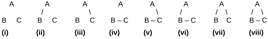
Consider a problem in network inference. There are three nodes, A, B, and C. Nodes are connected

by edges, and edges have no direction (e.g. A connected to B is the same as B connected to A). We

will rule out redundant edges and self-connections. For these three nodes, the full set of possible

networks is shown in Figure 1.

A priori, we have no idea which is the correct network. We might choose to reflect this in a prior

(19)

Network: P(network):

i 1/8

ii 1/8

iii 1/8

iv 1/8

v 1/8

vi 1/8

vii 1/8

viii 1/8

On first sight this is reasonable. For example, if the data at hand provide no information at all, then

the likelihood function will contribute nothing, and our posterior distribution is the same as our

prior – we still have no idea which is the correct network.

However, this sensible-seeming prior on networks implies a very different prior on the number of

edges per node in the network, as follows:

Connections per node in the network: P(connections per node)

0 1/8

1/3 3/8

2/3 3/8

(20)

Now, if our data contribute nothing to our views, after the analysis we are left believing that a

network with 2/3 of an edge per node is three times more probable than a network with 1 edge per

node.

To fix this, we might instead set the prior not on network topology, but on edges per node in the

network. We could set this prior as follows:

Connections per node: P(connections per node):

0 1/4

1/3 1/4

2/3 1/4

1 1/4

However, this then implies an unequal prior on network topologies:

Network: P(network):

i 1/4

ii 1/12

iii 1/12

iv 1/12

v 1/12

vi 1/12

vii 1/12

(21)

We may choose to place the uniform prior on the aspect of the network that most interests us.

However, this is certainly influencing other aspects of the result, which may be of interest to other

researchers; and may cause unease even within our own study.

The general impossibility of priors representing a total state of ignorance ‘across the board’ is a

fundamental aspect of Bayesian statistics, appearing even in single-parameter problems when we

consider transformations (Fisher 1956, 16-17; Edwards 1992, 58-60; Gelman et al. 1995, 56). For

example, perhaps we wish to make inferences about the area of squares. We will measure edge

length and from this calculate area, and will use a uniform prior. However, a uniform prior on edge

length implies a quadratic prior on area; a uniform prior on area leaves us with a square-root prior

on edge length. One solution is to abandon the prior entirely, and base all inference on the

likelihood function. This is equivalent to the smallest conceivable prior on all aspects of the solution

simultaneously, and in fact is the likelihood approach.

Priors in phylogeny reconstruction

Typically, Bayesian phylogeny reconstruction software uses a uniform prior on tree topology

(Holder and Lewis 2003). At first glance, this is a sensible representation of our total ignorance,

prior to performing the phylogeny reconstruction, as to which possible topology is correct.

However, it is clade existence which we are usually interested in, as reflected in the typical use of

posterior probabilities for clades in reported results (not probabilities for entire tree topologies). As

is now well documented, a uniform prior on topology implies a non-uniform prior on clade size,

with large and small clades more probable than clades of intermediate size (Pickett and Randall

(22)

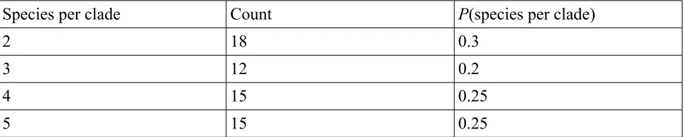
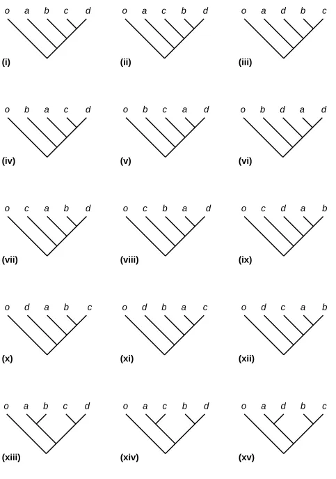
tree topologies. In Figure 2, for convenience, these are shown rooted with the same species as

outgroup. A uniform prior across these topologies – i.e. a prior probability of 1/15 for each topology

– implies a non-uniform prior on clade sizes (Table 2). Bayesian phylogeny reconstruction for five

species is then predisposed to find clades of size two more than clades of size four, and clades of

size three least of all.

Different priors on topology may be used, with the aim of greater biological realism. However,

since the actual processes underlying the tree are not known – we do not have a situation along the

lines of a ‘well shuffled pack of cards’, and never will – the prior will necessarily remain

controversial. Indeed, attempts to define a plausible prior (e.g. Velasco 2008) may simply shift the

problem, from a direct prior on topology to priors on the parameters of the model generating the

prior on topology (Autzen 2011). An analogy may be drawn to Fisher’s long-term but ultimately

unsuccessful quest for a general method to make uncontroversial, direct probability statements

about a parameter, known as fiducial inference (Fisher 1935b; Fraser 1968; Zabell 1992). Fiducial

inference was cast in non-Bayesian terms but may be regarded as an attempt to find entirely

uncontroversial, ‘uninformative’ priors (Seidenfeld 1992). Either this is impossible, or we do not yet

have the intellectual means to achieve it.

Topology is only one aspect of a phylogeny reconstruction. Priors are also required on branch

lengths and all other parameters of the model of evolution, for example substitution rates and

residue frequencies if they are allowed to vary. For example, an exponential prior for branch lengths

may be reasonable when substitutions are modelled as a continuous-time Markov process (but cf.

Ekman and Blaalid 2011). Even if this is accepted, what should the mean of that prior distribution

be? For Bayesian phylogeny reconstruction, a mean is required and it does matter (Yang and

(23)

Although the Bayesian approach provides a useful mechanism to incorporate prior knowledge

(Huelsenbeck et al. 2002), in practice we do not have prior knowledge of a sufficiently detailed

kind. Our prior knowledge tends to be straightforward and categorical, for example that the ingroup

is monophyletic (e.g. Buschbom and Barker 2006). Such knowledge can be incorporated into any

method of phylogeny reconstruction as a simple constraint on the tree topology. There is no

theoretical reason to introduce the additional baggage of having to propose a distribution on all

aspects of the phylogeny reconstruction problem, predisposing our inference towards certain results

in a way that is not obvious. However, for complex models a likelihood approach may be

impossible. Where the area of research seems to demand such models, this is a strong incentive to

use a Bayesian rather than a likelihood approach (e.g. Thorne et al. 1998; Drummond et al. 2006;

Huelsenbeck et al. 2006; Rannala and Yang 2007).

Model selection for maximum likelihood phylogeny reconstruction

The likelihood principle applies to a model whose mathematical structure is fixed. How do we

select this model structure in the first place? For phylogeny reconstruction by a conventional

maximum likelihood or Bayesian approach, a model of DNA or protein substitution is required. We

could specify a single model based on non-statistical criteria, or alternatively select one among a

range of models on statistical grounds. For selecting a substitution model, the topology of an initial

phylogenetic tree is obtained by some rapid means; a range of models is fitted to this topology by

maximum likelihood; one model among them is chosen, according to a criterion based on its

(24)

Likelihood alone cannot be used for model selection, except for a restricted set of models that have

the same number of free parameters. This is because adding a parameter to a model can only

increase the model’s explanatory power, hence increase its likelihood. For a range of hierarchical

models, the most complicated model would always be selected. Yet the most complicated model

may suffer from ‘overfitting’ – that is, paying too much attention to details that prove irrelevant.

To avoid overfitting, then, for likelihood-based model selection we require some concept of

‘penalty’ for extra parameters. Various penalties, or ‘rates of exchange’ between number of

parameters and improvement in likelihood, have been proposed. Edwards (1992, 199-202) notes

that ‘a fixed rate of exchange … can lead to paradoxes’, but suggests 2 units of log likelihood (ln L)

might be a good starting point in some cases. The Akaike Information Criterion or AIC (Akaike

1974) suggests 1 unit of ln L. With the Bayesian Information Criterion or BIC (Schwartz 1978), the

penalty depends on the amount of data. BIC’s penalty for additional parameters increases as the

sample size increases. Where pairs of models are hierarchical, a classical statistical approach is also

possible. One may treat the simpler model as representing a null hypothesis, the complex model as

representing an alternative hypothesis, and obtain a p-value from the likelihoods using a likelihood

ratio test (Wilks 1938).

As well as violating the likelihood principle, a likelihood ratio test seems unsuited to selecting a

model of substitution. Here, a substitution model is required, but there is no strong basis for

defining any one model as a null hypothesis. For selecting among a range of models without

resorting to a significance test, AIC and BIC both have justifications, but may conflict. Prior to

statistical model selection, we could reduce the size of the problem by using biological criteria to

the extent possible. For phylogeny reconstruction, for DNA sequences, does it make sense to accept

(25)

frequently used (e.g. the general time-reversible model). However, by the base-pairing rules within

the DNA double helix, we know that an A-to-G substitution on one strand implies a T-to-C

substitution on the other (and so on, for all possible substitutions). Such arguments do not point us

to a single model. For example, the model of Zagordi and Lobry (2005) and the simpler model of

Jukes and Cantor (1969) both conform to theoretical expectations from base-pairing rules. A further

selection procedure, beyond the realm of the likelihood principle, must still be applied (whether

statistical or subjective). Biological criteria have shown promise in phylogeny-based prediction,

where results could be evaluated according to known data (Barker et al. 2007).

Overall, the problem of model selection is not solved. Model selection occupies the interface

between extra-mathematical concerns (which models are we even willing to consider?) and

mathematical concerns (which model has best statistical fit to the data?), and is expected to remain

controversial. The matter is further discussed by Posada and Buckley (2004).

Case study: dating nodes on a phylogeny

In the previous section, I was optimistic about use of biological criteria to constrain models.

However, biological criteria may also lead us to models of such complexity that they are intractable

in the likelihood framework. Dating nodes on a phylogeny provides an example. Early stages of an

attack on the dating question are possible with a likelihood approach but, as yet, it appears the later

stages are not. The central problem is the confounding of time and of evolutionary rate. Where two

sequences have diverged greatly, we might infer either a long time since the divergence event, or a

(26)

Within the likelihood framework, it is straightforward to estimate branch lengths on the assumption

of a molecular clock acting across the phylogeny, and to test the extent of evidence for violation of

this assumption (Felsenstein 1981; Yang 2006, 226-228). If the assumption is sound, we might

regard branch length from the clock-assuming model as proportional to time. Further, where dates

of some nodes on the phylogeny are known, time and rate may be separated, providing estimates of

divergence times even where there are several molecular clocks operating within different parts of

the phylogeny (Yoder and Yang 2000; Yang and Yoder 2003). Assignment of branches to rate

categories must be known or assumed, or else may be performed by a heuristic approach dependent

on autocorrelation among nearby branches (Sanderson 1997). These likelihood and heuristic

methods do not incorporate uncertainty in the ‘known’ dates of nodes, though this uncertainty is

biologically relevant (Graur and Martin 2004; Shields 2004; Rannala and Yang 2007). Bayesian

approaches, in contrast, can incorporate uncertainties in dates (Yang and Rannala 2006) and varying

rates across the tree without user assignment of branches to categories (Drummond et al. 2006;

Yang 2006, 245-257; Rannala and Yang 2007). On one level, this provides exactly what we would

hope for: a realistic model incorporating uncertainty. However, this comes at a price. For example,

Yang and Rannala (2006, 214-215) ‘describe a method that enables the researcher to incorporate

any statistical distribution to describe uncertainties in the age of a calibration node and leave it to

the individual to choose an appropriate prior for the problem at hand’. The Bayesian approaches to

dating remove obvious problems such as point-estimates of node dates, which are unrealistic, but

introduce the new problem of which priors to use. In practice, the prior can have a strong influence

(27)

Time travel / waiting for the aliens

Two final thought experiments are these. Firstly, going forward another 130 years, how will our

methods and analyses look? Secondly, if aliens landed and turned out to have higher intelligence –

say, as different from ours as ours as ours is from apes’ – how laughable would our attempts at

statistical inference seem?

Research should be open and not fraudulent. Within these constraints, I suggest that an

over-emphasis on drawing strictly correct conclusions will doom us to humiliation. Even now, before the

future or the aliens have arrived, we know that most published papers are wrong (Ioannidis 2005).

With an emphasis on the less definable concept of intellectual progress, however, there is hope. For

example, Lamarck (1809) proposed a detailed mechanism of evolutionary change which was wrong

in every important respect. On the other hand, Lamarck recognised the earth as old and evolution as

real. His attempt to bring biology within the realm of universal laws (along the lines of physics;

Pichot 1994) launched an ambitious research programme which is still incomplete.

I suggest that, of the three statistical approaches it is likelihood – ‘clean’ on extra-mathematical and

axiomatic grounds though not always practical – that will stand out most positively to the aliens and

the people of the future. This should be recognised as partly an aesthetic decision, with which some

(28)

Conclusion: what should we do?

For a problem of inference such a phylogeny reconstruction, where there is no very obvious way to

construct an empirical prior, on theoretical grounds Bayesian inference seems the wrong approach.

Mathematically, Bayesian inference is fine and works. It also has the immense attraction of giving a

posterior probability distribution for hypotheses – giving us a mathematically sound view of the

certainty of our inference. However, a subjective prior is usually required, and this may not be

defensible in all respects (e.g. Felsenstein 2004, 288-305). My suggestion is, where technically

feasible, to abandon the prior entirely – which is to say, use a likelihood approach. Since this is

based on extra-mathematical arguments, others will disagree and it is perhaps safer to ‘leave [these

problems] as an exercise for the reader’ (Huelsenbeck and Bollback 2007, 484). Certainly, I do not

expect to uncontroversially and unambiguously solve a major problem in statistics in this, or any

References

Akaike, H (1974) A new look at the statistical model identification. IEEE Trans Autom Control
AC19:716-723
Altschul SF, Madden TL, Schäffer AA, Zhang J, Zhang Z, Miller W, Lipman DJ (1997) Gapped
BLAST and PSI-BLAST: a new generation of protein database search programs. Nucleic Acids Res
25:3389-3402
Anismova M, Gascuel O (2006) Approximate likelihood-ratio test for branches: a fast, accurate, and
powerful alternative. Syst Biol 55:539-552
Autzen B (2011) Constraining prior probabilities of phylogenetic trees. Biol Philos 26:567-581
Baldi P, Brunak S (2001) Bioinformatics: the machine learning approach, 2nd edn. MIT Press,
Cambridge
Barker D, Meade A, Pagel M (2007) Constrained models of evolution lead to improved prediction
of functional linkage from correlated gain and loss of genes. Bioinformatics 23:14-20
Beaumont MA, Rannala B (2004) The Bayesian revolution in genetics. Nat Rev Genet 5:251-261
Berger JO, Wolpert RL (1984) The likelihood principle. Institute of Mathematical Statistics,
Birnbaum A (1962) On the foundations of statistical inference. J Am Stat Assoc 57:269-306
Birnbaum, A (1972) More on concepts of statistical evidence. J Am Stat Assoc 67:858-861
Bühlmann P, van de Geer S (2011) Statistics for high-dimensional data: methods, theory and
applications. Springer, Berlin
Buschbom J, Barker D (2006) Evolutionary history of vegetative reproduction in Porpidia s.l.
(lichen-forming Ascomycota). Syst Biol 55:471-484
Casella G (1985) An introduction to empirical Bayes data analysis. Am Stat 39:83-87
Dos Reiss M, Zhu T, Yang Z (2014) The impact of rate prior on Bayesian estimation of divergence
times with multiple loci. Syst Biol 63:555-565
Douady CJ, Delsuc F, Boucher Y, Doolittle WF, Douzery EJP (2003) Comparison of Bayesian and
maximum likelihood bootstrap measures of phylogenetic reliability. Mol Biol Evol 20:248-254
Drummond AJ, Ho SYW, Phillips MJ, Rambaut A (2006) Relaxed phylogenetics and dating with
confidence. PLoS Biol 4:e88
Durbin R, Eddy SR, Krogh A, Mitchison G (1998) Biological sequence analysis. Cambridge
Edwards AWF (1977) R.A. Fisher’s work on statistical inference. In Parenti G (ed) I fondamenti
dell’inferenza statistica. Università degli Studi di Firenze, Firenze, pp 117-124. Reprinted in
Edwards (1992), pp 245-251
Edwards AWF (1992) Likelihood, expanded edition. John Hopkins University Press, Baltimore
Efron (2003) Robbins, empirical Bayes and microarrays. Ann Stat 31:366-378
Ekman S, Blaalid R (2011) The devil in the details: interactions between the branch-length prior
and likelihood model affect node support and branch lengths in the phylogeny of the Psoraceae.
Syst Biol 60:541-561
Felsenstein J (1981) Evolutionary trees from DNA sequences: a maximum likelihood approach. J
Mol Evol 17:368-376
Felsenstein J (1985) Confidence limits on phylogenies: an approach using the bootstrap. Evolution
39:783-791
Felsenstein J (2004) Inferring phylogenies. Sinauer, Sunderland
Firth D (1993) Bias reduction of maximum likelihood estimates. Biometrika 80:27-38
Fisher RA (1935a) The design of experiments. Oliver and Boyd, Edinburgh
Fisher RA (1956) Statistical methods and scientific inference. Oliver and Boyd, Edinburgh
Fraser DAS (1968) Fiducial inference. In Sills L (ed) International encyclopedia of social sciences.
The Macmillan Company and The Free Press, New York, pp 403-406
Gandenberger G (2014) A new proof of the likelihood principle. Br J Philos Sci.
http://dx.doi.org/10.1093/bjps/axt039
Gelman A, Carlin JB, Stern HS, Rubin DB (1995) Bayesian data analysis. Chapman and Hall,
London
Graur D, Martin W (2004) Reading the entrails of chickens: molecular timescales of evolution and
the illusion of precision. Trends Genet 20:80-86
Guindon S, Gascuel O (2003) A simple, fast, and accurate algorithm to estimate large phylogenies
by maximum likelihood. Syst Biol 52:696-704
Guindon S, Dufayard J-F, Lefort V, Anisimova M, Hordijk W, Gascuel O (2010) New algorithms
and methods to estimate maximum-likelihood phylogenies: assessing the performance of PhyML
3.0. Syst Biol 59:307-321
Holder M, Lewis PO (2003) Phylogeny estimation: traditional and Bayesian approaches. Nat Rev
Huelsenbeck JP, Bollback JP (2007) Application of the likelihood function in phylogenetic analysis.
In: Balding DJ, Bishop M, Cannings C (eds), Handbook of statistical genetics, vol 1, 3rd edn.
Wiley, Chichester, pp 460-488
Huelsenbeck JP, Larget B, Miller RE, Ronquist F (2002) Potential applications and pitfalls of
Bayesian inference of phylogeny. Syst Biol 51:673-688
Huelsenbeck JP, Jain S, Frost SWD, Kosakovsky Pond SL (2006) A Dirichlet process model for
detecthing positive selection in protein-coding DNA sequences. Proc Natl Acad Sci USA
103:6263-6268
Ioannidis JPA (2005) Why most published research findings are false. PLoS Medicine 2:e124
Jukes TH, Cantor CR (1969) Evolution of protein molecules. In Munro HN (ed), Mammalian
protein metabolism, vol 3. Academic Press, New York, pp 21-132
Kadane JB (2011) Principles of uncertainty. CRC Press, Boca Raton
Kahneman D (2012) Thinking, fast and slow, paperback edition. Penguin Books, London
Keane TM, Creevey CJ, Pentony MM, Naughton TJ, McInerney JO (2006) Assessment of methods
for amino acid matrix selection and their use on empirical data shows that ad hoc assumptions for
Kempthorne O (1962) Comments on A. Birnbaum’s “On the foundations of statistical inference”. J
Am Stat Assoc 67:319-322
Kumar S, Filipski AJ, Battistuzzi FU, Kosakovsky Pond SL, Tamura K (2012) Statistics and truth in
phylogenomics. Mol Biol Evol 29:457-472
Lamarck J-BPAM (1809). Philosophie zoologique. Dentu, Paris
Lim J-H, Iggo RD, Barker D (2013) Models incorporating chromatin modification data identify
functionally important p53 binding sites. Nucleic Acids Res 41:5582-5593
Lindley DV (1957) A statistical paradox. Biometrika 44:187-192
Lv J, Liu H, Huang Z, Su J, He H, Xiu Y, Zhang Y, Wu Q (2013) Long non-coding RNA
identification over mouse brain development by integrative modeling of chromatin and genomic
features. Nucleic Acids Res 41:10044-10061
Mayo D (2010) An error in the argument from conditionality and sufficiency to the likelihood
principle. In: Mayo D, Spanos A (eds) Error and inference: recent exchanges on experimental
reasoning, reliability, and the objectivity and rationality of science. Cambridge University Press,
Cambridge, pp 305-314
Nielsen R, Yang Z (1998) Likelihood models for detecting positively selected amino acid sites and
O’Meara BC (2012) Evolutionary inferences from phylogenies: a review of methods. Ann Rev Ecol
Evol Syst 43:267-285
Pagel M (1999) The maximum likelihood approach to reconstructing ancestral character states of
discrete characters on phylogenies. Syst Biol 48:612-622
Pichot A (1994) Présentation. In: Lamarck JBPA, Philosophie zoologique, avec présentation et notes
par André Pichot. Flammarion, Paris, pp 7-49.
Pickett KM, Randle CP (2005) Strange bayes indeed: uniform topological priors imply non-uniform
clade priors. Mol Phylogenet Evol 34:203-211
Posada, D (2008) jModelTest: phylogenetic model averaging. Mol Biol Evol 25:1253-1256
Posada D, Buckley TR (2004) Model selection and model averaging in phylogenetics: advantages
of Akaike information criterion and Bayesian approaches over likelihood ratio tests. Syst Biol
53:793-808
Randle CP, Pickett KM (2010) The conflation of ignorance and knowledge in the inference of clade
posteriors. Cladistics 26:550-559
Rannala B, Yang Z (2007) Inferring speciation times under an episodic molecular clock. Syst Biol
Royall R (2000) On the probability of observing misleading statistical evidence. J Am Stat Assoc
95:760-768
Sanderson MJ (1997) A nonparametric approach to estimating divergence times in the absence of
rate constancy. Mol Biol Evol 14:1218-1231
Schwarz G (1978) Estimating the dimension of a model. Ann Stat 6:461-464
Seidenfeld T (1992) R.A. Fisher’s fiducial argument and Bayes’ theorem. Stat Sci 7:358-368
Shields R (2004) Pushing the envelope on molecular dating. Trends Genet 20:221-222
Simmons MP, Norton AP (2013) Quantification and relative severity of inflated branch-support
values generated by alternative methods: an empirical example. Mol Phylogenet Evol 67:277-296
Sober E (2008) Evidence and evolution: the logic behind the science. Cambridge University Press,
Stamatakis A (2014) RAxML version 8: a tool for phylogenetic analysis and post-analysis of large
phylogenies. Bioinformatics 30:1312-1313
Thorne JL, Kishino H, Painter IS (1998) Estimating the rate of evolution of the rate of molecular
evolution. Mol Biol Evol 15:1647-1657
Tuffley C, Steel M (1997) Links between maximum likelihood and maximum parsimony under a
simple model of site substitution. Bull Math Biol 59:581-607
Tversky A, Kahneman D (1974) Judgement under uncertainty: heuristics and biases. Science
185:1124-1131
Velasco JD (2008) The prior probabilities of phylogenetic trees. Biol Philos 23:455-473
Wilks SS (1938) The large-sample distribution of the likelihood ratio for testing composite
hypotheses. Ann Math Stat 9: 60-62
Yang Z (2006) Computational molecular evolution. Oxford University Press, Oxford
Yang Z, Rannala B (2005) Branch-length prior influences Bayesian posterior probability of
phylogeny. Syst Biol 54:455-470
Yang Z, Rannala B (2006) Bayesian estimation of species divergence times under a molecular clock
using multiple fossil calibrations with soft bounds. Mol Biol Evol 23:212-226
Yang Z, Yoder AD (2003) Comparison of likelihood and Bayesian methods for estimating
divergence times using multiple gene loci and calibration points, with application to a radiation of
Yang Z, Kumar S, Nei M (1995) A new method of inference of ancestral nucleotide and amino acid
sequences. Genetics 141:1641-1650
Yoder AD, Yang Z (2000) Estimation of primate speciation dates using local molecular clocks. Mol
Biol Evol 17:1081-1090
Zabel SL (1992) R.A. Fisher and the fiducial argument. Stat Sci 7:369-387
Zagordi O, Lobry JR (2005) Forcing reversibility in the no-strand-bias substitution model allows
for the theoretical and practical identifiability of its 5 parameters from pairwise DNA sequence
Tables
Hypothesis, H Likelihood, P(D|H) Prior probability, P(H) Posterior probability, P(H|D)
Librarian high x k.x.(high value)
Farmer low > 20x > k.20x.(low value)