Estimation of Inefficiency using a Firm specific Frontier Model

Estimation of Inefficiency using a

Firm-specific Frontier Model

Das, Arabinda

Acharya Prafulla Chandra College

13 April 2013

Online at

https://mpra.ub.uni-muenchen.de/46168/

Arabinda Das1 Department of Statistics

Acharya Prafulla Chandra College

Kolkata – 700 131

India

Abstract

It has been argued that the deterministic frontier approach in inefficiency measurement has a

major limitation as inefficiency is mixed with measurement error (statistical noise) in this

approach. The result is that inefficiency is contaminated with noise. Later stochastic frontier

approach improves the situation with allowing a statistical noise in the model which captures

all other factors other than inefficiency. The stochastic frontier model has been used for

inefficiency analysis despite its complicated form and estimation procedure. This paper

introduced an extra parameter which estimates the amount of proportion that an error

component shares in the observational error. An EM estimation approach is used for

estimation of the model and a test procedure is developed to test the significance of presence

of the error component in the observational error.

Keywords: stochastic frontier model, skew-normal distribution, identification, EM algorithm,

Monte Carlo simulation.

JEL Classification: C15, C21, C51

1_{Address for correspondence: Arabinda Das, Assistant Professor, Department of Statistics, Acharya Prafulla Chandra College, New}

2

1 Introduction

In early twentieth century, Cobb and Douglas (1928) introduced the econometric estimation

of production function for estimating the economic efficiency of a firm using given inputs

and a technology. They used the ordinary least square (OLS) method of estimation to

estimate the production function which requires the observations to lie around it. This

assumption, however, contradicted the theoretical definition of production function which

refers to the maximum (frontier) output attainable using a given inputs and a technology.

Next thirty years econometric analysis of production function ignored this frontier property of

the production function and was primarily based on the estimated ‘average’ production

function.

Winsten (1957) was perhaps first to attempt estimation of the frontier production function

using Corrected OLS (COLS) method. In this method, the intercept of the OLS estimated

‘average’ production is adjusted so that all the observations lie below the estimated

production function. Aigner and Chu (1968) suggested the estimation of production function

using linear and quadratic programming technique with the frontier restriction i.e. the

residuals are to be positive. However, this approach has two main drawbacks. Firstly, it is

deterministic as there is no stochastic specification and, hence, one cannot compute the error

margin of the estimates and ii) The estimates were found to be very sensitive to outliers.

Timmer (1971) suggested an iterative approach to overcome these problems where at each

stage a new deterministic frontier is estimated after deleting those data points with respect to

which the estimates at the previous stage were found sensitive and the process is continued

until the deterministic frontier function stabilizes. Richmond (1974) improved upon the

COLS estimates to make them unbiased and consistent.

Schmidt (1976) estimated the deterministic frontier model with a statistical sense by the

maximum likelihood method assuming error with a one-sided distribution like exponential

and half-normal. The resulting estimates under these distributional assumptions are

equivalent to the linear and the quadratic programming estimators of Aigner and Chu (1968).

Later, Greene (1980) estimated another deterministic frontier model assuming errors are

gamma variables.

Although the deterministic frontier approach of Aigner-Chu-Schmidt estimates the frontier

function respecting its frontier property, an obvious limitation of this approach is that in this

approach one cannot isolate the effect of inefficiency from that of the random noise as both

3

regularity conditions required for application of ML method viz. the support of the

distribution of y must be independent of the parameter vector. In this approach the regularity condition is violated. One can, however, apply the MOLS method of Richmond (1974) which

is a combination of the OLS and MOM, for estimation of the parameters of the deterministic

frontier.

The stochastic frontier approach introduced by Aigner, Lovell and Schmidt (1977), Meeusen

and van den Broeck (1977) and Bettese and Corra (1977) overcomes the limitations of the

deterministic frontier approach by decomposing the disturbance term into two random

components representing the “random noise” and the “inefficiency”. While the decomposition enables one to separate out the effects of random noise from the inefficiency

and makes the support of the distribution of output independent of the parameter space, the

concept of stochastic frontier ensures the frontier restriction on the observed outcomes. The

stochastic frontier model is the extension of deterministic frontier model with added

stochastic noise. However, sensitivity of the stochastic frontier model depends on

mis-specification and amount of statistical noise and inefficiency in composite disturbance.

Ruggiero (1999) examined the performance of deterministic and stochastic frontier models

using Monte Carlo simulation experiments. The analysis revealed that the deterministic

frontier model was more consistent than stochastic frontier model. Also, deterministic

frontier model outperformed the stochastic frontier model which concludes that the stochastic

frontier model does not decompose the stochastic noise and inefficiency correctly.

Measurement error leads to bigger biases in the stochastic frontier model than it does in the

deterministic model. This suggests that the main criticism against the deterministic models is

hypocritical.

The purpose of this paper is to provide a more general frontier model which is specific to

each firm. An extra binary random variable is introduced to decide whether a deterministic

frontier or stochastic frontier model is appropriate for each firm.

The rest of the paper is organized as follows. Section 2 presents the more general stochastic

frontier model and derives the distribution of the observational error. Section 3 presents the

estimation procedure to estimate the parameters of the model. In section 4, a Monte Carlo

experiment is constructed to compare the performance and the results of the analysis and their

implications are reported. In section 5 we report and analyze the results of an empirical

application of the firm-specific frontier model. The major conclusions emerging from this

4

2 A Firm-specific Frontier Model

Let yi and xi be the output and vector of non-stochastic inputs of the ith firm respectively

indexed by the production function f(.) and ei be the random error. Then a firm-specific

frontier model for the ith firm can be presented as

y_i f x( , )_i b e_i; e_i J v_{i i} u_i , i 1,...,n (2.1)

where b is a vector of unknown parameters to be estimated. The random error ei is

composed of two unobservable stochastic terms viz. vi, the statistical noise and ui 0, the

technical inefficiency and Ji is a unobservable binary random variable that defines whether

the frontier model is stochastic frontier or deterministic frontier for ith firm. If Ji 0, the

frontier model becomes deterministic frontier model and if Ji 1, the frontier model

becomes stochastic frontier model.

The distribution of error component vi can be assumed to be normal i.e.

2

(0, )

i v

v N s and

the distribution of error component ui can be assumed to be half-normal (ALS, 1977) or

Exponential (Stevenson, 1980) or Gamma (Greene, 1990) with ui 0. We retain these

distributional assumptions regarding the error components in this paper. Also it is assumed

that Ji Bern( )p .

The density function of ei can be found as:

Let j e1( )i is the density function of ei when Ji 0 and j e2( )i is the density function of ei

when Ji 1. Then, the density function of ei is given by

f( )ei pj e2( )i (1 p j e) ( )1 i . (2.2)

The density function of ei can be considered as a two component mixture model. The EM

algorithm can be most reliable approach to estimate the parameters of the model using the

density function of ei.

2.1 Estimating firm-specific inefficiency

Though the primary objective of the frontier model is to estimate the unknown parameter

5

firm-specific inefficiency in the firm-specific frontier model are the Jondrow et al. (1982)

proposed conditional mean or mode of u given which is given by

E u( | )i ei g( , )e di (2.3)

which is a function of the unknown parameter vector and the observational error and can be

estimated using the estimated value of parameter vector and the observed data. This measure

of inefficiency given in (2.3) can be computed using the conditional distribution of u given e. In our model the conditional distribution of u given e can be derived as follow:

The conditional distribution function of u given e can be derived as

( | ) ( | , 0) ( 0) ( | , 1) ( 1)

P U u e P U u e J P J P U u e J P J

P U( u u| )p P U( u u| v)(1 p)

pF u( ) (1 p) ( |F u u v)

Then the conditional distribution of u given e can be derived by differentiating the above equation by u as

( | )f u e pf u( ) (1 p) ( |f u u v)

Therefore the Jondrow, et al. (1982) measure of firm specific inefficiency is given by

E u( | )e pE u( ) (1 p) ( |E u u v) (2.4)

In ALS (1977) the error components vi and ui are assumed to be distributed as normal and

half-normal respectively i.e. v N(0,sv2) and

2

(0, u)

u N s with ui 0.

Under these assumptions, when Ji 0, ei ui and the density function of ei is given by

2

1 2

2 1

( ) ( ) exp 2 2

i i i

u u

f e j e e

s ps

(2.5)

and similarly when Ji 1, ei vi ui the density function of ei is given by

2

2 _{2 2} 2 2 2 2

2 1

( ) ( ) exp

2 2

u i i

i i

v u v u v

u v

f e j e s e e

s s s s s

p s s (2.6)

which is a skew-normal density (Azzalini, 1985).

Under these specific assumptions, the Jondrow, et al. (1982) measure of firm specific

inefficiency is given by

( | ) 2 (1 ) ₂ ( / )

1 ( / )

i i

i i u

i

E u e p s p sl f e l s e l

p l e l s s (2.7)

where

u v

6

2 2

u v

s s s

Now, the posterior estimate of probability of a firm being stochastic is given by

( | ) ( | ) ( 1, ) ( )

i i

i i i i

i

P J

E J P J

P

e

e e

e

( | 1) ( 1) ( )

i i i

i

P J P J

P e e 2 2 1 ( ) ( , ) ( ) (1 ) ( )

i

i i

i i

pj e

g e d

pj e p j e (2.8)

This g e di( , )i can be termed as the responsibility of randomness of ith firm. The estimates in

equation (2.8) can be estimated using the maximum likelihood estimator of the parameter

vector d, dˆ and the estimated residuals eˆ_i. These posterior estimates of inefficiency are firm

specific and provide us the probability of a firm’s randomness given the input vectors and a

technology.

3 EM Estimation of the Model

The log-likelihood of the model is given by

log ( ; ) log[ ₂( , )i (1 ) ( , )]₁ i i

L d y pj y d p j y d

The maximum likelihood estimators can be found by solving log ( ; )Ld y d 0. Trying to

maximize log ( ; )L d y directly for the estimation of parameters is quite difficult since those

equations are nonlinear and no analytic solutions can be found. So numerical procedure like

iterative optimization methods often be used to get successive approximation of the solution.

In that case The EM algorithm is applied to estimate the parameters of the model. The model

is recasted into a missing data framework in order to implement the EM algorithm. The

unobserved binary variable J can be treated as the missing data and the observable output y

can be treated as observed data. Then the complete data is given by (y, J). The density

function of Ji is given by

1

( ; ) Ji(1 ) Ji

i

f J p p p .

Now see the joint density of the observed data e and unobserved data J:

1 1 2

1

( , ) ( ) ( | ) (1 ) ( ) i ( ) i

n

J J

i i

i

f e J f J f e J p j e pj e (3.1)

Then from (3.1) the joint density of the observed data y and unobserved data J can be

obtained by the transformation '

y x

7

₁ 1 ₂ 1

( , ) ( ) ( | ) (1 ) ( ) i ( ) i

n

J J

i i

i

f y J f J f y J p j y pj y

The complete log-likelihood function of the complete data (y,J) is given by

log ( ; , ) (1 i) log[(1 ) ( )]1 i ilog[ 2( )]i

i i

L d y J J p j y J pj y

Since, the values of Ji is unknown, so we want to use the expected value of Ji|yi to

substitute each J i in above. We have

( | ) ( | ) ( 1, ) ( )

i i

i i i i

i

P J y

E J y P J y

P y

( | 1) ( 1) ( )

i i i

i

P y J P J

P y 2 2 1 ( ) ( ) ( ) (1 ) ( )

i i i i y y y pj g d

pj p j

The expected value of Ji|yi is called the responsibility of the model for ith observation,

denoted as ( )g di :

g di( ) E J( i| , )yi d

Then the Q-function, which is the expected value of complete log-likelihood with respect to the conditional distribution of J given y, is given by

( ) J y| [log ( ; , )] J y| (1 i) log[(1 ) ( )]1 i J y| ( ) log[i 2 ( )]i

i i

Q d E L d y J E J p j y E J pj y

(1 _i( )) log[(1 ) ( )]_{1 i i}( ) log[ ₂( )]_i

i i

y y

g d p j g d pj

log(1 ) (1 i( )) (1 i( )) log ( )1 i log i( ) i( ) log 2( )i

i i i i

y y

p g d g d j p g d g d j

(3.2)

Under the assumptions of ALS (1977), the density functions of ei under the assumption of

deterministic frontier model and stochastic frontier model are presented in (2.5) and (2.6)

respectively.

Then, the log-likelihood function under the assumption of deterministic frontier model is

given by

1 2 2 ' 2

1 1

log ( ) log ( )

2 2

i u i

u

y c y x

j s b

s (3.3)

8

'

2 2 ' 2

2 _{2 2} 2 2

1 1

log ( ; ) log( ) log ( )

2 2( )

u i

i u v i

v _{u v} u v

y x

y c s b y x

j d s s b

s _{s s} s s (3.4)

Therefore, from (3.2) and using (3.3), (3.4) the Q-function is given by

2 ' 2

2

1 1

( ) log(1 ) (1 ( )) (1 ( )) log ( ) log ( )

2 2

i i u i i

i i u i

Q d p g d g d c s y xb p g d

s

'

2 2 ' 2

2 2

2 2

1 1

( ) log( ) log ( )

2 2( )

u i

i u v i

i v _{u v} u v

y x

c s b y x

g d s s b

s _{s s} s s

4 Monte Carlo Evidence

A Monte Carlo simulation experiment is carried out to study the finite sample properties of

the estimators under the generalized SFM. The model that is used for the experiment is a cost

frontier model with one output produced by one input which is given below:

yi b₀ b₁xi J vi i ui (4.1)

where J Bern( )p u N (0,su2) and

2

(0, v)

v s . Let '

0 1

( , , v, u, )

h b b s s p . A random

sample on y can be generated using a simulation procedure from the distribution of e by the

transformation ei yi b₀ b₁xi for a given value of h h0. The density function of ei can

be considered as a two component mixture model. The first component is normal distribution

with right truncation and a random sample from this distribution can be generated by inverse

method. The second component is the skew-normal distribution and a composition method of

marginal-conditional can be used to generate a random sample from this distribution.

Therefore, a random sample of size n on y can be generated using the above algorithm using a specified value of p. The composition method of marginal-conditional can be derived with a

given h₀, as a single observation, say ith observation, of u, is first generated by the marginal distribution of u where u is distributed as half-normal variate. Given the value of ui as

obtained, ith observation on e can be found by the conditional distribution of e given u

which is normal and then ith observation on y using the relation yi b00 b10xi ei. The

above two steps are repeated n times to generate a random sample of size n on y.

9

repeated 100 times. The cross sectional sample of size n = 100, 200, 300, 400, 500 are considered for the study.

Under this Monte Carlo experiment, the parameter vector h, is estimated using the EM

algorithm, describe above, to compare the small sample behavior of the parameter vector h.

The result is reported in table 1. The analysis provides the mean, SD and RMSE of the

estimators.

The complete data expected log-likelihood equations were solved by the BHHH algorithm

fixing the tolerance at 0.001. For each replication the EM method converged at reasonably

fast rate taking about three minutes in a PENTIUM-4 processor. The mean, SE and the root

mean square error (RMSE) of the estimates for each experiment, obtained from their

generated sampling distributions, are reported in Table-1. It is seen that for lower values of n

the performance of the EM estimates as measured by standard error and the RMSE is poor

and the number of iterations for convergence moderately high. However, the performance

improves, as n is increased from 150 to 400 when estimates stabilize. Interestingly the

number of iterations required for convergence of the EM algorithm decreases by almost

one-third as n is increased from 150 to 500. At n=500, the small sample error of the EM estimates

are between 6 to 10 per cent. Given the fact that the single equation estimates of the SFM

suffer from simultaneous equation bias, the small sample performances of EM estimates of

our model is reasonably good.

5 Empirical Analysis

We have used the US electricity utility industry data (Greene 1990, Table-3) to illustrate the

method. The model to be fit is a cost function rather than a production function, given by

2

0 1 2 3 4

ln(cost Pf) b b ln( )Q b ln ( )Q b ln(P Pl f) b ln(P Pk f) u J v

where Q is the output, a function of labor (l), capital (k), fuel (f), and Pl, Pk and Pf are their

respective factor prices; and u N (0,su2), v N(0,sv2); u truncated at zero. It may be

noted that the change in the expression for e requires that e u should now be replaced by

u

e in the above derivations.

We have estimated two models. The SFM with independent error components is estimated

using maximum likelihood method with BHHH algorithm. The other firm-specific frontier

model discussed above with independent error components is estimated using the illustrated

10

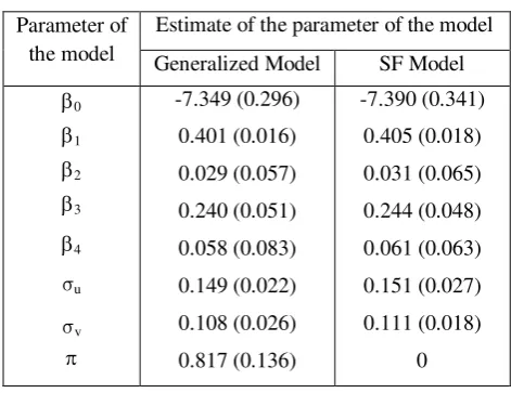
the Table-2. It can be seen from the Table-2 that the regression coefficients of the

uncorrelated components SFM have significantly higher asymptotic variance than the

firm-specific frontier model which is estimated by EM algorithm. Also, the estimated value of the

parameter  is 0.817 which is statistically significant and suggests that almost 81% firms

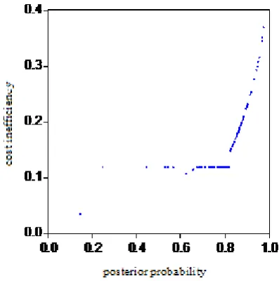
prefers stochastic frontier model whereas 19% firms prefers deterministic frontier model. Fig.

1 presents measures of firm-specific cost inefficiency in the firm-specific frontier model. Fig.

2 presents the estimated posterior probability of randomness.

6 Conclusions

In this paper we have proposed a firm-specific frontier model where each firm is open to

choose between stochastic and deterministic frontier model. This generalized model is

estimated using EM estimation method. It is seen that the EM method does not face the

problems like divergence, instability and low. The results of Monte Carlo simulation

experiments show fairly good small sample properties of the EM estimates. Application of

the model to the cross-section data of 123 US electricity firms shows stochastic frontier

model is preferable to almost 81% firms and deterministic frontier model is preferable to

remaining 19% firms.

References

Aigner, D. C. and S. F. Chu (1968) On Estimating the Industry Production Function.

American Economic Review, 58:4, 826-839.

Aigner, D., K. Lovell and P. Schmidt (1977) Formulation and Estimation of Stochastic

Frontier Production Function Models, Journal of Econometrics, 6, 21-37.

Azzalini A. (1985) A Class of Distributions which includes the Normal Ones, Scand. J.

Statistics, 12, 171-178.

Battese, G. and G. Corra (1977) Estimation of a Production Frontier Model with Application

to the Pastoral Zone off Eastern Australia. Australian Journal of Agricultural Economics, 21, 169-179.

Cobb, C. and P. H. Douglas (1928) A Theory of Production. American Economic Review,

Supplement, 18, 139-165.

Greene, W. H. (1980) On the Estimation of a Flexible Frontier Production Model. Journal of

11

Greene, W. H. (1990) A Gamma Distributed Stochastic Frontier Model. Journal of

Econometrics, 46, 141-164.

Jondrow, J., I. Materov, K. Lovell and P. Schmidt (1982) On the Estimation of Technical

Inefficiency in the Stochastic Frontier Production Function Model, Journal of Econometrics, 19, 233-238.

Kumbhakar, S., and K. Lovell (2000) Stochastic Frontier Analysis, Cambridge University Press, Cambridge.

Meeusen, W. and J. van den Broeck (1977) Efficiency Estimation from Cobb-Douglas

Production Functions with Composed Error, International Economic Review, 18, 435-444. Pal, M. (2004) A note on a unified approach to the frontier production function models with

correlated non-normal error components: the case of cross-section data, Indian Economic

Review, 39, 7–18.

Pal, M. and A. Sengupta (1999) A model of FPF with correlated error components: an

application to Indian agriculture, Sankhya B, 61, 337–50.

Richmond, J. (1974) Estimating the Efficiency of Production, International Economic

Review, 15:2, 515-521.

Ruggiero, J. (1999) Efficiency Estimation and Error Decomposition in the Stochastic Frontier

Model: A Monte Carlo Analysis. European Journal of Operational Research, 115:3, 555-563.

Schmidt, P. (1976) On the Statistical Estimation of Parametric Frontier Production Functions.

Review of Economics and Statistics, 58:2, 238-239.

Stevenson, R. (1980) Likelihood Functions for Generalized Stochastic Frontier Estimation.

Journal of Econometrics, 13, 57-66.

Timmer, C. P. (1971) Using a Probabilistic Frontier Production Function to Measure

Technical Efficiency. Journal of Political Economy, 79:4, 776-794.

Winsten, C. B. (1957) Discussion on Mr. Farrell’s Paper. Journal of the Royal Statistical Society, Series A, 120:3, 282-284.

Wu, C. F. J. (1983) On the convergence properties of the EM algorithm, The Annals of

12

Table 1: Results of the Monte Carlo simulation experiments

0 1

( , , v, u, )=(1, 0.1, 0.1, 0.1, 0.5)

h b b s s p

n EM Estimate

Mean SD RMSE 100 1.224

0.079 0.136 0.146 0.594 0.134 0.141 0.135 0.218 0.245 0.202 0.135 0.143 0.227 0.291 200 1.158

0.087 0.138 0.135 0.557 0.121 0.127 0.118 0.183 0.228 0.159 0.133 0.121 0.224 0.247 300 1.113

0.091 0.121 0.129 0.546 0.096 0.098 0.097 0.123 0.185 0.129 0.111 0.112 0.149 0.213 400 1.109

0.093 0.118 0.116 0.532 0.087 0.082 0.092 0.111 0.145 0.114 0.092 0.104 0.128 0.167 500 1.110

0.095 0.107 0.112 0.528 0.082 0.076 0.089 0.092 0.118 0.109 0.087 0.102 0.114 0.120

Table 2: Estimates of the parameters

Parameter of the model

Estimate of the parameter of the model

Generalized Model SF Model

13

Fig 1: Kernel density of estimated cost inefficiency

Fig 2: Kernel density of estimated posterior probability