Spatiotemporal Cattle Data—A Plea for Protocol Standardization

Spatiotemporal Cattle Data—A Plea for Protocol

Standardization

Dean M. Anderson

, Rick E. Estell

, Andres F. Cibils

1_{United States Department of Agriculture, Agricultural Research Service, Las Cruces, USA;} 2_{Department of Animal and Range}

Sci-ences, New Mexico State University, Las Cruces, USA. Email: *_{[email protected]}

Received December 11th_{, 2012; revised January 15}th_{, 2013; accepted January 24}th_{, 2013}

ABSTRACT

It was not until the end of the 1990’s that animal born satellite receivers catapulted range cattle ecology into the 21st

century world of microchip technology with all of its opportunities and challenges. With the global navigation satellite

system (GNSS), insight about how cattle use a landscape is being revealed from previously unknown temporal and spa-

tial behaviors. The most common system to date for studying ungulate movement is the global positioning system

(GPS). With its use has come a clarity and completeness in documenting spatial and temporal data in new and exciting

ways that offer almost unlimited possibilities to better understand and manage economic and societal returns from ani-

mal dominated landscapes. However, its use on free-ranging cattle is not without challenges, some of which are yet to

be optimally solved. To maximize the usefulness of GNSS data, consideration must be given to: 1) developing a stan-

dardized protocol for reporting and analyzing research that facilitates interpretation of results across different ecosys-

tems; 2) develop optimum ranges over which to collect satellite fixes depending upon the particular behaviors of inter-

est; and 3) concurrently develop electronic hardware and equipment platforms that are easily deployed on animals and

that are light, robust, and can be worn by cattle for extended periods of time without human intervention (e.g., changing

batteries). Once data are collected, appropriate geographic information system (GIS) based models should be used to

produce a series of products that can be used to implement flexible management strategies, some of which may support

methodologies that are yet to be commercialized and adopted into future plant-animal interface management routines.

Keywords:

Cattle Behavior; Animal Tracking; GPS

1. Introduction

Free-ranging animal behavior is challenging to study and

manage in light of the more than 68 factors that have

been shown to influence it [1]. Obtaining both accurate

and precise cattle behavior data is essential to understand

and subsequently manage free-ranging animals. Of the

40 different behaviors cattle can engage in [2], 95% of

them can be classified into one of four main activities:

foraging, walking, standing, or lying [3]. Foraging is

probably of greatest interest to most land stewards be-

cause of the impact it has on animal dominated land-

scapes, especially when these landscapes are required to

supply goods and services beyond providing adequate

nutrition for free-ranging animals. Therefore, studying

animal-to-animal variability is basic to understanding

free-ranging animal behavior [4].

The official study of animal behavior did not become

part of agricultural college curricula until the late 1950’s

[5]; however, the importance of behavior was recognized

in husbandry texts dating back to the 1800’s [6]. Focused

livestock behavior research in the USA began in the

1920’s. Early studies such as those of Sheppard [7] and

Cory [8] relied entirely on eyesight and hand written re-

cordings to document the behaviors observed. Thereafter,

sight and stop-watches remained the sole tools for docu-

menting free-ranging animal behavior for many years [9].

Today observation still remains a powerful and useful

tool for documenting free-ranging animal behavior [10-

16]; however, it has limitations especially during periods

of darkness [3] and following extended periods of con-

tinuous observation when fatigue can accentuate ob-

server bias [17]. Furthermore, the mere presence of an

observer can impact both wildlife [18] and domestic

animal [19,20] behaviors. The question then becomes

“how is the observer influencing the observation?” The

answer to this question is not trivial and frequently is not

provided by researchers who do not describe protocols to

minimize its potential bias in behavioral studies [21].

an observer and the animal being observed. Observing

from parked vehicles [22], horseback [23] or platforms

positioned above the ground [24] have been used.

Though sampling methods exist for observational data

[25], there is as yet no tool available that can overcome

human inefficiency when multitasking [26], a prerequi-

site for observing and recording data from more than one

animal at a time.

Furthermore, to overcome human sight limitations,

binoculars [27] as well as night vision technologies [28,

29], video recordings [30] and even lasers [31] have been

employed. As early as the 1950’s, electronics were used

to track wildlife [32]. Because of their lead, wildlife re-

searchers established many of the guidelines used through-

out the 20th century for tracking domestic animals. One

of the earliest attempts to augment observations of cattle

behavior with electronics was a biotelemetry system de-

veloped by Australian researchers in the 1970’s [33]. For

a complete discussion of electronics in wildlife tracking

the reader is directed to texts by Kenward [34] and Mill-

spaugh and Marzluff [35]. Currently no textbooks exist

to assist range-animal ecologists in developing protocols

for monitoring free-ranging livestock using 21st century

technologies. This review traces the application of the

global navigation satellite system (GNSS) [36,37] for

tracking free-ranging cattle with a focus on its

imple-mentation and the challenges range animal scientists face

when deploying GNSS to study free-ranging cattle be-

haviors.

2. A Satellite Based Technology

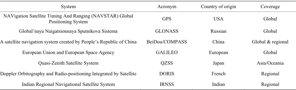
The GNSS can be traced back to 1966 as described in the

Woodford/Nakamura Report [38,39]. Of the several sat-

ellite-based systems being used or developed today [40,

41]; (see

Table 1

) the most familiar tracking system is

the NAVigation Satellite Timing And Ranging (NAVS-

TAR) System [42] commonly referred to as the global

positioning system (GPS) [43].

Contrary to some versions of GPS, this utility was de-

veloped initially for both military and civilian users [37].

The technology is robust with respect to electric trans-

mission lines [44] yet GPS signals are very weak at the

surface of the earth making them susceptible to interfer-

ence and jamming [45] as well as potentially being vul-

nerable to spoofing [46].

Research using GPS-based telemetry systems for

tracking animals began in 1991 [47]. Six years later,

cows were monitored for the first time using this tech-

nology [48]. Since 1997, at least 99 studies have been

reported in which GNSS devices have been used to

monitor free-ranging cattle behavior (

Table 2

). Being

able to characterize animal behavior data within a spatial

as well as a temporal context with respect to peers and

the landscape is a major benefit provided by GNSS data

[16,49]. In addition to monitoring spatial and temporal

information, GNSS technology has been combined with

other electronics to monitor free-ranging animal health

[50] and numerous other behaviors associated with for-

aging and moving [51]. Most studies employing GNSS

have attached the devices directly to the free-ranging

animal; however, cows can be successfully tracked by a

person moving with cattle that carries a GPS unit [52-

54].

3. GNSS Devices

Applying GNSS technology to free-ranging animals is

expensive and remains a major challenge when designing

studies to track free-ranging cattle [56]. A sheep was the

first domestic ruminant on which a GNSS device was

deployed at a cost exceeding $47,000 per unit in 2011

US dollars [55]. The first commercially available GPS

units could cost between $2500 and $5000 [47]. In 2012

the price of individual GNSS devices ranged between

$500 and >$3000 per animal, with low cost units typi-

cally being non-commercial tracking devices not spe-

cifically designed for tracking animals [57].

Most biologists/ethologists and technicians are not

skilled in reading electronic schematics or performing

electronic assembly, let alone attending to electronic

maintenance. However, for those with this expertise on

their team and 4 to 5 hours of time that can be devoted to

build a GNSS tracking device, the Clark animal tracking

system (ATS) [58] may be the most user friendly pack-

age currently available, since a detailed bill of materials

is available at http://clark.nwrc.ars.usda.gov/collars/.

Other hand built GNSS tracking devices have been de-

scribed in the literature [57,59] but instructions for their

assembly are less detailed than that provided for the

Clark ATS. An alternative to purchasing devices specifi-

cally built to track free-ranging animals is to purchase a

commercial GNSS device designed for recreational pur-

poses that can be attached to an equipment platform de-

signed to be worn by free-ranging animals. Several re-

searchers [30,48,57,60-67] have adapted various models

of Garmin GNSS products while the Magellan 315 has

also been successfully used [68]. Several researchers

have also used GNSS devices incorporated into elec-

tronic systems manufactured either by individuals [69] or

university departments or research organizations with

electronic/computer engineering expertise [16,70-81].

For those who choose to use commercial equipment de-

signed specifically for free-ranging animals, a number of

companies are listed on the World Wide Web. To date,

the company whose products have been used most often

to monitor cattle (

Table 2

) is headquartered in Newmar-

Table 1. The global navigation satellite system (GNSS).

System Acronym Country of origin Coverage

NAVigation Satellite Timing And Ranging (NAVSTAR) Global

Positioning System GPS USA Global

Global’naya Naigatsionnaya Sputnikova Sistema GLONASS Russian Global

A satellite navigation system created by People’s Republic of China BeiDou/COMPASS China Global & regional

European Union and European Space Agency GALILEO European Global

Quasi-Zenith Satellite System QZSS Japan Asia/Oceania

Doppler Orbitography and Radio-positioning Integrated by Satellite DORIS French Regional

Indian Regional Navigational Satellite System IRNSS Indian Regional

based on GNSS technology [82].

One of the greatest advantages of on-site assembly of

GNSS devices vs. commercial products is reduced “down-

time” during equipment failure. When commercial equip-

ment fails, it normally cannot be repaired on site and

must be returned to the manufacturer. This can interfere

with data collection. One method to address equipment

failure is to have back-up units available for deployment

when GNSS devices fail. Though it increases the initial

cost of a project, this approach seems reasonable; yet

none of the studies reported in

Table 2

specifically indi-

cated this was a part of their experimental protocol.

Though GNSS equipment failure may not occur when

devices are deployed on free-ranging animals [83], this is

the exception rather than the rule (see

Table 2

). Future

GNSS animal tracking manuscripts should publish fail-

ure rates as well as reasons or suspected reasons for fail-

ure. This information will assist future behavior-based

GNSS research to develop protocols that can minimize

data loss as well as providing information useful to com-

mercial companies seeking to manufacture more robust

models of their equipment [42,84]. Resolving equipment

failures quickly is important because incomplete GNSS

data sets result in poor statistical inferences [85]. How-

ever, it has been suggested that GNSS data sets with

<10% missing data can be safely analyzed to determine

habitat-selection [86].

4. Number of Cattle to Instrument

No studies to date have been conducted to determine

exactly how many animals within a group need to be

instrumented to accurately describe the group behavior

being investigated. Differences exist even among identi-

cal twin dairy cattle [4] so it is no surprise that more than

one GPS instrumented animal is needed to accurately

describe behaviors such as grazing within a group of cat-

tle [87]. Animal to animal variability exists in wildlife

species [88] as well as domestic cattle [12] and this vari-

ability may be quite large depending on the individual

animal behaviors of interest. Therefore, research is need-

ed to determine what percentage of a herd should be in-

strumented to accurately describe herd behavior [79].

Cattle behave gregariously in groups, which has been

cited as justification for instrumenting only a few ani-

mals [89]; however, very large discrepancies in behavior

among individual(s) within a herd have been reported

[49]. The problem of adequate sample size has been ex-

acerbated by satellite tracking technology because of the

expense of GNSS units [90]. Though determining num-

ber of animals to instrument will probably always be

linked to cost and though a sample size of 6 to 12 sub-

jects should be considered low, this number may be

suitable for well-planned experiments based on correla-

tional evidence [91]. As few as four steers grazing a 0.16

ha irrigated paddock were able to accurately categorize

grazing, ruminating and idling with observation periods

between 15 and 30 minutes [92]. Management recom-

mendations regarding watering location have been advo-

cated based on GNSS data from only two cows [93].

However, it is safe to assume that most foraging animals

only behave “normally” when held in groups [94].

Significant error can be introduced by characterizing

landscape utilization patterns with data from only a few

animals. Location errors were found to increase from

10% when four of five cows were used in a model to

40% when only a single cow was used [49]. Therefore, it

might be concluded that many of the studies in

Table 2

Table 2. Ranking of 99 free-ranging cattle studies beginning in 1997 through 2012 that have employed global navigation sat- ellite system (GNSS) technology. Blank cells indicate data not provided by the author(s) and could not be calculated from manuscript.

Materials and Methods

Total GNSS Device

Fix rate

R

eferen

ce [#]

Study location Paddock size

Herd composition Herd si

ze

Ca

ttle

instr

ume

nte

d

Inst

rum

ent

s

Inst

rum

ent

fai

lu

re

How instr

ume

nte

d c

attle

c

hose

n

1

Time between down

-load

s

Model

Atta

ch

me

nt

3

Devi

ce m

ass

Manufactur

er

2

(Min./fix) Correct

ed

4

Ba

tte

ry

lif

e

Analysis Tools Accur

acy

ha No. No. No. No. or (%) Days kg Days m

48 Cow/calf _pairs 16 7 a _{GPS receiver}VP-On Core a 2 a Visual Basic &

Intergraph’s MGE product

suite 1 - 2

210 6 Cows 7 7 5

49 paddocks 16 each 0.378

Cow/calf pairs

+ steers 8 + ≤16 7 58 (29) b GPS_2000 b < 1 5 to 360 a 10

ArcView GIS V 3.0 within 895%

23

48˚21'29"N; 109˚34'31"W & 48˚21'29"N;

109˚34'31"W

245 & 330 Cow/calf _pairs 159 81 7 to ₁₂ Variable a 3 to 7 b 2200 b 5 to 30 Chi-square _procedures 5 to 12

180 119₄₃˚_˚43'W; _29'N >825 Cow/calf _pairs 40 6 15 (19 to 79) on _{2 of 6 collars} a 21 b b 1.15 20 a 1.9 ± S.E. _0.24

69 465.5 A cow 1 1 1 b 2 to 5 c Prototype III _{V. 2} c 0.5 to 1 b

156 31.38583_97.40944˚_˚N; _W 40.5 to 43.1 Cow/calf pairs & steers

11 & 16 4 or 5 & 3 19 to ₄₁ ≈60 b 2000 b 2.5 & 5 a 7 to 14 & _{4 to 6 dissertation}See

165 2 & 3 Steers 4 & 6 to 8 2 or 3 15 b GPS 2200 b 5 MINITAR® Statistical Software

191 _cattle Beef 16 or 17 18 b 5 ArcGIS

202 119₄₃˚_˚43'W; _29'N 810 Cows 120 _treatment 4 per 6 b 2000 b 10 REPEATED

with the MIXED procedure of

SAS

154 38₈₄˚_˚02'N; _36'W 2 to 3 Sub-set 126 b GPS_2200 b 5 a Two way repeated measures

0.02- advertised horizontal

159 ₁₀₉48˚20'42"N; _˚35'59"W 337 Cow/calf _pairs 160 9 6 a 8 to 22 b 2000 b 5, 10 & 20 a Sufficient Mixed model _ANOVA 5 - 12

101 14₃˚_˚25'N; _26'E Cows 14 b >0.5 d GeoExplorer II d 5.5 0.167 a Discriminate analysis PROC

DISCRIM & SAS 8.1

2 to 5

68 Cows

15 14

13 c 1 e 315 b

104 38₈₄˚_˚02'N; _36'W 2 to 3 Cows & _steers 126 b GPS_2200 b 5 a SAS Proc _MIXED published 0.002 = horizontal

172 33₈₃˚_˚24'N; _29'W 14.20 & _17.52 Cow/calf _pairs 20 & 20 3 & 3 a 8 b GPS 2200 LR b 5 a

Nonparametric PROC UNIVARIATE

(SAS) 3

60 f GPS 18 LVC e 3.4 4 c 7 < 3

Continued

211 USA = 119˚43'W;

43˚29'N; Israel = 35˚35'E; 32˚55'N

USA = 825 to 859; Israel = 28

Cows & cow/calf pairs

USA = 40; Israel = not given

USA = 6;

Israel = 7 16 a b USA = 2000; Israel = 2200

LR b USA =

1.15; Israel =

1.35 USA = 5;

Israel = 5 USA = a; Israel = b discriminationRegression &

160 ₁₀₉48˚_˚21'42"N; _35'46"W 78 to 176 Cows 5 to 7 a ≈14 b 2000 b 15 a 3 to 10 fixed model Mixed & ANOVA

± 7

164 2 to 3 Cows 36 15 42 a 20 b GPS_2000 b 0.95 5 a Kernal home _range

168 32₃₅˚_˚55'N; _35'E 27.5 & _28.2 Cows 41 4 to 6 12 17 to 25 b 2200 b 5 ArcView 3.2

70 Cows 14 8 57 Up to (33) f eTrex b + belt ≈ 1.8 0.033 b < 1 Mean = _1.8

176 ≈435 to ₁₄₇₆ Cows & _stockers 4 Numerous 3 to 74 g L 400 b 15 c 54

DataTraxTM_,

ArcViewTM

3.3 & 9.1, Hawth’s Analysis Tools 3.21

±8

181 ₁₁₉43˚28'30.77"N; _˚40'29.77"W 13 to 14 _cows Dry 20 12 60 a 7 b 2200 b 10 a Microsoft _Qbasic 4.1 ± 0.39

103 14˚25'N;

3˚26'E 29,800 Cows 194 12 6 b 0.5 d GeoExplorer II d 0.4 0.167 a 0.5 ArcGIS 3.2 & SAS 8.1 2 to 5

205 ₁₁₉37˚04'N; _˚43'W 193 Cows 8 to 14 a b 2200 LR & _{3300 LR} b 15 a ANOVA & KRESS

Modeler ≤ 2

157 ₁₀₉48˚_˚21'47"N; _36'29"W 123 to 167 _cows Dry 133 to 214 4 to 6 35 a 4 b 2000 b 10 a ≤ 4 Categorical _modeling 5 to 7

167 5.91 Cattle 11 4 30 6 h GPS plus-4 b 0.233 40 GIS software Open source “Open Jump” 10 61 12.1 Cows 15 12 f GPS 18 LVC e 0.33 c 4.5 ArcMap < 3

177 4 a b & g 3300 LR & _{L 400} b 15 c & d 70 GPS Host & _DataTraxTM ± 5

182 ₁₁₉43˚_˚29.4'N; _42.7'W >800 Cow/calf _pairs 60 4 per 20 20 a 15 b 2200 b 5 a 5.5

187 ₁₃₁16˚49'S; _˚13'E 900 to ₅₇₀₀ 2 to 4 per _paddock ≈180 b 60 ≈180

Home Range extension for ArcView & ArcGIS 9.1 & Kernel analysis

96 106₃₂˚_˚43.263"W; _34.297"N 466 Cows c 0.717 to _0.883 b K-means _classifier

208 ₁₄₅20˚30'S; _˚58'E 1530 Cows & cow/calf

pairs 183 12 7 (25) a 56 g L 400 b 30 Sptial Analyst in ArcMap 9.1

161 ₁₀₉48˚_˚21'47"N; _36'29"W 258 & 329 _cows Dry 195 18 9 4 a 40 b 2200 b 10 a PROC MIXED _{& % time} Within 7

162 ₁₁₀46˚37'N; _˚36'W 600 Cow/calf _pairs 42 to 59 4 to 5 9 a 27 to 29 b 2200 b 15 a _square Latin Within 7

158 48˚21'47"N; 109˚36'29"W 258 to 359

Dry cows 160

4 to 8 per group, total = 45

28 a 64 b 2200 b 10 a 7

166 ₁₀₅34˚_˚15'36"N; _24'36"W 146 & 219 Pregnant _cows 77 & 88 16 19 d 5 to 7 b 3300 b a ArcView 3.3, 9.0 & PROC MIXED

173 Heifers ≈600 18 3 1 b 3300 b 5 & 15 a 3 to 5

174 ₁₀₀29˚_˚15'0.02"N; _5'54.01"W 1211 Cows 9 12 b 3300 LR b 5 a ArcView ≤ 5

183 Ranch A = 76; Ranch B = 193; Ranch C = 400

Cows A =15 B = 40 to 70, C = 70

A = 15, B = 5 to 8, C = 8

(11 to 100)

A = 1, B = 24 to 30, C = 21

A = ? B & C = b

A = unknown, B = 2200 LR,

Continued

184 12 Cows 6 paddocks × 15 cows = 90

1 per paddock 7

Technical challenges

14 per

paddock g AGTraXTM b 10 ArcGIS 9.1 & SAS GLM procedures

186 13₅₈˚_˚21'E; _42'N 18 _calves Heifer 28 h GPS Plus 2 b 0.25 b _{SAS Mixed}ArcMap &

188 ₁₁₉43˚29'N; _˚43'W 829 to 864 Cow/calf _pairs 60

3 paddocks × 4 cows

= 12 20 (9) a 15 b 2200 LR b 5 e

Global Mapper v. 6.06 & Idrisi32 v. 32.22

190 1 Heifers 6 to 8 3 43 7 b 5 Excel, Minitab _{15 & ArcGIS}

71 long. 150.3897125; lat. −23.213914 1.25

Bulls &

cows 18 & 36 18 (50 to

100) (20 to 44) 0.083 i FleckTM b 0.0167

89 1.5 Dairy _cows 60 3 5 e g TU 400 b 1 ANOVA & chi-squared goodness-of-fit

Within 5

62 53₁₀˚_˚37'N; _12'E 180 Cows 74 3 4 ≈304 f _Venture eTrex b 2.1 5

ArcView 3.1 & multiple linear regression

72 150˚13'E;

23˚8'S 7 Cows 6 (2 to 6)

lost fixes 3.65 i FleckTM 2 b 0.0042

Gamma probability

density function

212 Cows 21 - 23 b 3300 LR b 5

155 35₃₂˚_˚35'E; _55'N 22 & 34 Cows & _steers 24 & 18 b & j

b = 2200; 3300 j = not

given b b = 5 j = 1

Multiple regression 7

63 _animals Herded Cows & _bulls 45 to 250 10 7 f eTrex Legend f 0.25 0.63 to _0.75 OziExplorer_Software TM 15

179 33₈₃˚_˚24"N; _29"W Cow/calf _pairs 20 15 to 18 83 a 13 to17 b 2200 LR b 5 a ArcView GIS 3.2 and SAS PROC MIXED 3

73 7 6 4 i FleckTM _{b 0.004}

Hidden Markov Model

& long-term prediction algorithm

74 150₂₃˚_˚13'E; _8'S 21 Cows 36 3 i FleckTM _{b 0.004}

194 Cows & cow/calf pairs

2 to 20 cows per

herd

6 30 5 to 7 b 2200 LR and _{3300 LR} b 5 ArcGIS

75 Heifers 27 21 i FleckTM _{b Paired t-test}

197 27₈₁˚_˚09'N; _12'W 19.0 to _22.1 Cows 1 to 4 per _paddock (0 to 24) 5 b GPS_2200 b 0.95 15 a

ArcView & Animal Movement Extension

< 5

209 ₁₄₆20˚34'S; _˚07'E 93 to 117 Steers 3 a 42 g L 400 b 30 & 60 2 × 2 factorial

163 ₁₀₆32˚32'N; _˚48'W 1002 to ₃₇₇₀ Cow/calf Cows & pairs

7/group total = 21

1 per group &

total = 3 a 8 to 10 k & b WTI GPS

500 b & 3300 b 30 & 10 a

Repeated measure of PROC MIXEDWithin 7

77 40˚18'S;

175˚50'E 0.5 Heifers 20 8 40 6 l b ≤ 10 6 to 8 4.7 static

78 11 Cow/calf _pairs 50 12 24 6 d Lassen iQ b 1.28 10 b 4 to 6 4.7 static

169 32₃₅˚_˚55'N; _35'E 76 to 135 Cows 17 9 to 11 50 4 b 2200 b 5 ArcView 9.1

170 50˚N; 114˚W Cattle 9 b ≈127 b 60

ArcView 9.2/ & Hawth’s

Spatial Analysis Tools

Continued

64 1˚26'S; 35˚12'E

Herded animals

Cows &

bulls 6

GPS inadvertently

switched off, < (1)

f eTrex Legend f of cattle <0.01% mass

0.25 0.63 to 0.75

OziExplorerTM

Software 15

175 28₉₉˚_˚56"N; _51"W 948 to ₃₈₈₂ Cows 1000 cows & 7000

stockers 4 (1) f 70 g & b Not given & 3300 LR or

3300 S b 15 a 14 to 28 ArcGIS 9 and Hawth’s

Tools ± 5

178 paddocks 12 each1.1

Dairy cows

17 out of

180 17 9 b b

1 or movements

> 4 m

MINITAB 15 for Windows

185 42₉₃˚_˚00'N; _25'W 12.1 Cows 6 paddocks ×

15 cows = 90

1 per

paddock 7 ≈(7) paddock14 per g AGTraXTM b 10 ArcGIS 9.1 & SAS MIXED procedures

7.7 ± S.D. 1.32

189 _117.71045.130˚N; _˚W 56.4 to _101.2 Cows 10 a 12 b 0.0167 6.25 Microsoft®,

Excel®, Global Mapper®, &

ArcMap®

193 1200 to _{2300 & steers} Heifers 20 b 3300 L b 20 & a 10 or 30 daily cycle

Hawth’s Tools v. 3.26 in ArcGIS 9.2

Mean = 37

196 0.51 to _0.58 Dairy _cows 64 64 (100) <1 m Trackstick IITM _{b 0.0167} Proc mixed

SAS

30 _species Mixed Multiple 5 Descriptive 3 f _{Astro 220} DC 20 & g 0.17 0.05 14 MapSource, Garmin’s ArcGIS 9.3

65 14˚38’E; 50˚02’N 2.3

Cows & cow/calf pairs

15 15 f Foretrex 201 h 2.4 1 Cluster analysis (CLARA method) & R 2.6.0

1.5 to 7.8 m/min

static

79 147₃₁˚_˚31’E; _17’S Steers 360 3 1 11 n UNEtracker II b

ArcGIS & Microsoft Excel

99% within 20

80 Steers 220 6 3 10 n UNEtracker II b 5 b ArcGIS, Microsoft

Excel & Hawths

Tools

213 ₁₄₁42˚59’N; _˚24’E 2.2 to 2.8 Cow/calf _pairs 10 2 20 (2.8 to 3.9) b 10 o b 10 ArcGIS 9.0 & one-way ANOVA’s

215 Cow/calf _pairs 10 a l Clark ATS b 5 ESRI® ArcMApTM

9.3 & Hawths analysis Tools v 3.27

& Global Mapper v 9.03

57 42₉₃˚_˚00’N; _25’W 2.02 Cows 15 15 15 (80) in 4 da,

harness not

electronics 8 e GPS 18 LVC e 3.4 0.33 c 4.5 ArcMap

195 12 Cows 10 2 0.0167

198 ₁₀₆32˚_˚37’N; _40’W 2425 Cows 6 7 b 3000 b 5 a ARCGIS 9.1

199 Cows 14 p Tellus Basic _{5H2D v 2.0} p

200 2373 Cattle 500 26 to 52 ≈50 ≈114 to ₁₅₅

76 ₁₅₀23˚13’S; _˚23’E ≈7.6 Steers 32 32 32 ≈43 2 j FleckTM _{3 b 0.033 2}

Matlab 7.7, ArcGis 9.3 Hawth’s Analysis Tools 3.27

204 42˚00’N; 93˚25’W

6 × 12.1

paddocks Cows 95 1 to 2 per

paddock 2 Successive 14 g & q AgTraX &

Prototype b 10 b ArcGIS 9.1 Static evaluation

206 4.4 & 6.2 Cow/calf

pairs 14 14 7 g b 3

Continued

207 29˚18’S;

115˚7’E 21.5 to 64 Heifers 217 2 per paddock

= 6

3 (10 to 16) a g WildTrax b 5 14

ArcMap 9.2 & repeated- measures-

Genstat

106 48 to 322 Heifers 36 8 22 r _Terminal GPRS- b 0.35 60 ≈50 _{within 20}99%

95 ₃₃35_˚˚_01'N 5'E; 1.5 Cows 100 4 4 g 4 b 3300 LR b 5 b

ArcGIS 9.X with discriminant and partition analysis using

JMP v 7.0.2 software

216 Cow/calf _pairs 10 a 7 p Clark ATS b

16 106₃₂˚_˚41'W; _34'N 433 Cow/calf _pairs 30 & 12 5 & 12 40 only 2 devices per

year had

≥ (90) useful data

h 2 to 3 s _prototype Custom c 0.017 b 1 to 3 Python 2.6 & ArcGIS 9.3, SAS 9.2

81 13.5 to _125.2 Cows & cow/calf pairs

2 to 3 (10.9) a 5 to 14 t _prototype Custom b 1.65 10 _procedure MIXED

66 30₅₁˚_˚05'S; _40'W 3.0 to _5.2 Heifers 174 f eTrex i Trackmaker

Pro® Software

192 4 Cows 14 8 57 8 b 0.133

67 Two herds 7 Technical _failures i 1 f _{Astro 220} DC 20 & g 0.17 0.05

Garmin’s MapSource, ArcGIS 9.3, &

GraphPad Instat ver. 3.1

140 29˚15'N; 100˚5'W 29˚19'N; 99˚42'W 34˚15'N; 105˚24'W

Cows with & without calves

24 10

6 < (2.5) 21 21

60 b 3300 b 5 a ArcGIS 9.1 < 5

201 ₁₀₆32˚32'N; _˚48'W Cows _breed 2 per a b 3300 b 10 & 15

214 ₁₀₅34˚_˚15'36"N; _24'36"W 146 Cow/calf _pairs 18 18 18 g 7 b _{3300 LR} 2200 & b 5 a 30 ArcGIS 9.0 & SAS Cluster and Disc

1_{How instrumented cattle chosen: a = Randomly; b = Selected; c = Lead cow; d = Availability; e = Carefully chosen; f = Chute cut; g = Not random; h = Docile} disposition; i = Based on leadership; 2_{Manufacturer: a = Motorola; b = Lotek; c = Future Segue; d = Trimble; e = Magellan; f = Garmin}TM_{; g = Blue Sky} TelemetryTM_{; h = Vectronie-Aerospace GmbH; i = CSIRO; j = Trilogical; k = Wildlife Track Inc.; l = Custom; m = Telespial Systems; n = University of New} England; o = ATF Co. Ltd.; p = Televilt; q = Ames Laboratory; r = Telespor; s = MIT Computer Science and Artificial Intelligence Lab; t = Engineering Ser- vices Group; 3_{Attachment: a = Hand-made girth harness; b = Neck collar; c = Neck Saddle; d = Canvas backpack; e = Shoulder harness; f = Handmade collar} taped to cowbell; g = Harness; h = Girth Strap; i = Halter mount; 4_{Fix rate corrected: a = DPGS; b = None; C = WAAS; d = EGNOS; e = Lotek N4 v.1.1895} software.

requirements but the number of location fixes recorded

per unit of time can be reduced with software that will

“power down” the electronics when animals are not

moving [96]. Recently a hybrid system was developed

that employs a kinetically powered network of primary

and secondary nodes powered by the movement of an

animal’s neck. When these systems are combined with

GPS technology at specific locations, termed “hotspots”,

autonomous monitoring of free-ranging animals (reindeer

were the test subjects) may be economically feasible over

landscapes

≤ 2000 km

_{[97]. Future GNSS studies to}

determine the correct ratio of instrumented to non-in-

strumented animals required to accurately characterize

the behavior of interest among various landscapes are

needed.

5. Methods of Attaching GNSS Devices to

Cattle

recommendations have not been specifically reported for

cattle, GNSS data collection should be delayed at least a

few hours following instrumentation to allow animals to

adjust to the equipment. Again observation of the animal

after it is instrumented is necessary to determine the op-

timum time necessary for each animal’s personality to

accept wearing the equipment package. In sheep a 16 h

period between instrumenting an animal and the onset of

data collection appears to be adequate [102].

Regardless of the GNSS device used, the predominant

method employed for deploying GNSS devices on cows

has been neck collars (

Table 2

). However, girth har-

nesses or backpacks [48] and various shoulder harness

platforms have also been used [57,60,61,65,66,101,103].

Each equipment platform design has its own merits as

well as challenges. Equipping cows with neck collars is

an art in terms of placing the correct tension on the collar.

If the tension is too tight, skin abrasion can occur, but a

loose collar may slide over the cow’s head during graz-

ing or get caught on objects in the landscape. Further-

more, tension can affect the data quality if the electronics

package contains motion sensors capable of measuring

side-to-side and/or up and down movement of the head

and neck [104]. Mounting “differences” have been found

to affect sensor counts among collars [49]; this suggests a

protocol be developed for calibrating individual collars.

Magnetometer signals can differ based on hardware ori-

entation [51]. To address proper collar tension on cattle it

may be possible to use a neck collar composed of elastic

material that would stretch yet remain tight during de-

ployment to eliminate skin abrasion yet prevent slippage.

In a stretch design the belt material would have to be

capable of wicking sweat and moisture away from the

animal’s skin to minimize abrasion. An adjustable slip

noose collar has been designed for use on domestic

lambs and several wildlife species [105].

If a collar rotates such that the GNSS antenna is not

pointed skyward, GNSS fixes can be lost [24,70]. Even

though some non-skyward orientations of antennas may

allow GPS fixes to be captured, it will be less efficient

[106]. Most collar designs position the heaviest compo-

nents (usually the batteries) on either side of the neck to

act as counter balances [24,70] or allow batteries to

freely slide on a belt as the battery hangs below the ani-

mal’s neck [16] to help stabilize the GNSS antenna in a

skyward position. Another technique to help keep the

GPS antenna pointed skyward has been to attach a dense

foam rubber pad in the shape of an open “V” to the top of

the equipment box hanging below the cow’s neck to

prevent rotation [77]. When the collar is adjusted to the

proper tension, the cow’s neck fits into this “V” and re-

duces the tendency of the collar to swing from side-

to-side or rotate. The combination of head halters with

wide neck belts or saddles has also been used success-

fully to deploy GPS antenna on free-ranging cattle [16,

24,107].

The use of GPS tags in wildlife research [91], termed

bio-logging [108], is increasing and packaging GNSS

into ear tags for use on free-ranging cattle is currently

being advertised as a commercial reality. Reducing en-

ergy consumption [109], the need to reduce battery mass

[110] of an ear tag, and designing an antenna that is ro-

bust and always able to receive the GNSS signal [111]

are just three of the challenges. The earliest attempts to

place electronics in ear tags to be worn by cattle were not

successful because the studs used to attach a 113 g tag to

the cattle’s ear pinna were too short and caused abrasion;

however, by increasing the stud length to 3.81 cm and

drilling holes through the nylon washer that held the ear

tag in place, ear damage was eliminated [112]. More re-

cent research found ear tags weighing between 227 g and

250 g could only be tolerated for three to five days if

placed close to a cow’s head [110]. Reducing the mass

and increasing length of the button studs allowed feedlot

cattle to tolerate a 114 g tag for up to four weeks. How-

ever, for long term deployment ear tags should probably

not exceed 25 g [112].

6. Accuracy or Precision

Accuracy is not a fundamental characteristic of a dataset

but must be derived from outside itself; therefore, col-

lecting more GNSS data may not necessarily improve

accuracy but could actually decrease accuracy [113].

Furthermore, differential correction of GPS data (DGPS)

also contains errors with accuracy degrading at an ap-

proximate rate of 1 m for each 150 km distance the GPS

unit is from the reference station [114]. Not only do

methods for correcting GNSS data differ [115] but static

and dynamic accuracies differ [116,117].

It is ironic that most free-ranging animal studies in

which GNSS data are collected focus on the temporal

and spatial data of moving cattle yet accuracy figures

reported by most researchers refer to static accuracy

(

Table 2

). Furthermore, not all collars, even from the

interval of 15 s can result in 2.3 to 3.8 fixes per minute (P

< 0.001) depending on landscape terrain/obstructions, yet

differences in open terrain were negligible [123]. Meas-

ures of accuracy can be means or counts and accuracy

specifications should always state the metric used. This

relationship is complex because GNSS positions exist in

three dimensions yet knowing most locations in 2D (a

flat map) is adequate [124] (

Table 3

).

However, if 3D information is desired, then root mean

square (rms) vertical, twice the distance of the root mean

square (2drms) or spherical error probable (SEP) would

be a more appropriate set of statistics to consider. Most

often when accuracy is stated (e.g. 5 m), it is most likely

a circular error probability (CEP) which assumes GNSS

errors are Gaussian and have a circular distribution [124].

However, the shape of error distributions is a function of

how many satellites are being tracked and where they are

located in the sky. A more circular error pattern occurs

when more satellites are in view, whereas fewer satellites

create a more elliptical pattern and a corresponding

higher horizontal dilution of precision (HDOP). Both

autonomous and differential global positioning system

(DGPS) errors are approximately Gaussian, but because

GNSS errors are correlated in time, a stationary receiver

will produce errors that for one period of time may tend

to be in one direction and at a later period of time may be

in a different direction [124]. This is because the GNSS

signal is non-stationary [113]. The positional dilution of

precision (PDOP) is based on the number as well as the

geometry of the satellites available to the GNSS device;

the lower the PDOP number, the more accurate the GPS

fix. As more satellite systems (

Table 1

) [36,125] come

on line, the error distributions will become more circular

[124] which will benefit data accuracy and analyses.

Furthermore, GNSS users who require real-time data will

benefit from receivers using both GPS and GLONASS

data to lower PDOP. Using both GPS and GLONASS at

mid-latitudes can lower PDOP more than 15% and at

latitudes above 55

˚

PDOP could be lowered by as much

as 30% using both systems [41].

Unfortunately, many authors use precision and accu-

racy interchangeably when discussing GNSS though sta-

tistically they are distinctly different. Today we can track

animals with a precision never before possible using

GNSS [42]; however, determining GNSS accuracy re-

mains largely undocumented or possibly inappropriately

documented. The GNSS devices used in the studies listed

in

Table 2

usually either restated accuracy provided by

the manufacturer (most likely a static accuracy) or re-

stated accuracy cited in previous research using the same

model GNSS device. Only a few researchers have at-

tempted to determine GNSS accuracy of their devices

[118,122,126] and it was static accuracy they evaluated

and unfortunately static and dynamic accuracy are dif-

ferent [117]. Furthermore, most commercial suppliers

provide only static accuracy values [127]. The static ac-

curacy of GNSS devices has been reported to be between

0.01 m [128] and 15 m [129]. On May 2, 2000 at 12:00

AM when selective availability was deactivated, accu-

racy of GPS data improved substantially [130] and to-

gether with differential correction location error has now

been decreased from 80 m to 4 m [131]. Earlier methods

Table 3. Global Navigation Satellite System (GNSS) measures of horizontal accuracy in meters and their relationship for circular, Gaussian, and error distributions (adapted from [124]).

Statistics1

Root mean square dimensionalities2 _{Percent horizontal accuracy used in the cell phone industry}3

USA Japan

CEP4 _{= rms}

1 = rms2 = 67 = 95 = 68 = 98 =

1 0.85 1.19 1.26 2.08 1.28 2.37 CEP

1.18 1 1.41 1.49 2.45 1.51 2.80 rms1

0.84 0.71 1 1.06 1.74 1.07 1.99 rms2

0.79 0.67 0.95 1 1.64 1.01 1.88 67

0.48 0.41 0.58 0.61 1 0.62 1.14 95

0.78 0.06 0.93 0.99 1.62 1 1.85 68

0.42 0.36 0.5 0.53 0.88 0.54 1 98

1_{How to make conversions using this table. Horizontal statistics are the product of multiplying the vertical statistics by the appropriate cell value; an example:} rms2 = rms1 × 1.41; 2The square root of the one dimensional mean rms1 or North error and for rms2, the horizontal error representing the square root of the mean of the squared horizontal error; 2 drms is twice the horizontal rms, i.e., 2 drms = 2 × rms2; 3Refers to the radii of circles, centered at the antenna position con- taining between 67 and 98 percent of the points in a scatter plot; 4_{Circular Error Probable (CEP) refers to the radius of a circle, centered at the antenna position,}

that employed triangulation of Very High Frequency

(FHV) radio signals were in the range of 70 to 600 m

[126,132]. Reporting only the static accuracy of GNSS

devices is not totally correct since the major reason for

instrumenting cattle with GNSS devices is to improve

our understanding of their dynamic behaviors [133].

Furthermore, stationary collars may be as much as 33%

more successful at acquiring fixes than when deployed

on animals [134].

Though literature exists that describes how dynamic

testing of GNSS devices can be accomplished [116,117],

the testing of GNSS devices to be deployed on cattle

using this equipment will probably not be possible for

most ethologists. This quandary may have a relatively

simple solution. One approach would be to “etch” a pat-

tern into the soil surface or place something on the sur-

face that could be followed to delineate a pattern with

straight and curved segments (similar to a typical cattle

route). This pattern could be replicated in any ecosystem

for evaluating dynamic aspects of GNSS devices. The

length of this pattern would be based on the number of

GNSS fixes per unit of time. The devices could be car-

ried along the route either on foot or by an all-terrain

vehicle at a realistic walking speed for moving cattle (e.g.

≤3.2 km/hr; 2 miles/hour). This speed can be used to

gather cattle on the Jornada Experimental Range and

probably represents a maximum walking rate of travel

for cattle except for brief periods when they may run for

very short distances. The number of times required to

traverse the route would depend on a number of factors,

especially those influenced by the geometry of the satel-

lites in the sky and the rate at which GNSS fixes were

being recorded. If tree cover is a concern when actual

data collection takes place, tests should be performed

under both open and closed canopies. This protocol

would provide a measure of dynamic instrument-to-in-

strument precision among the devices to be deployed on

free-ranging animals. Furthermore, it would be possible

to calculate each instrument’s dynamic accuracy by

comparing the instrument’s data to data obtained using

survey grade GPS equipment to document the path’s

spatial location on the landscape.

Recent publications suggest the dynamic behaviors of

walking and foraging by cattle can be determined at

GNSS fix rates of <5 min [16,72,101]. Currently this is a

concern because most commercial GNSS devices have a

maximum fix rate of ≥5 min (

Table 2

). The reason for

the 5 min maximum fix rate among many commercially

available GNSS units for free-ranging animals is unclear

but most likely arose from the inability of wildlife re-

searchers to easily recapture animals to change batteries

and/or download data stored in memory. The need for an

increased GNSS fix rate for livestock studies may change

this industry norm. In the future it may be possible to

deploy GNSS devices for longer periods by using solar

[107,135] or kinetic [136] energy to recharge batteries,

though this is not presently a commercially practical re-

ality. Furthermore, data storage, once a challenge, is of

little concern today due to the ability to periodically

wirelessly transmit data back to a base station or to store

data on the animal using memory cards with substantial

memory [135].

7. GNSS Data, Maps and Analysis

The intent of this review is not to delve into the intrica-

cies of combining GNSS data with geographical Infor-

mation systems (GIS) data. However, scale and resolu-

tion must be considered when designing research in-

volving GNSS data. If GNSS data are to be plotted on

maps it is currently possible to purchase aerial satellite

photography with spatial resolution of 300 mm and with

images available in a number of spectral bands (

Table 4

).

If satellite spatial resolution is not adequate, cameras

fixed to remote controlled helicopters [137] or unmanned

aerial vehicles [138] can produce images with 1 mm and

30 to 60 mm resolution, respectively. The key is to de-

termine the scale necessary to evaluate the GNSS data

required to answer the question(s) being addressed and to

then plan research protocols accordingly.

Currently there is no off-the-shelf solution that com-

bines GNSS data with a GIS package, thus supporting

the need for providing adequate methodology detail

[139]. One of the most important uses of GNSS data is to

guide a researcher’s interpretation of what has taken

place on a landscape. Yet there remains a scale-depend-

ence of movement behavior that requires further refine-

ment [85].

Analysis of GNSS data after collecting it may be the

most poorly addressed aspect when using GNSS tech-

nology to monitor free-ranging cattle behavior. The fol-

lowing example helps to focus on this challenge. Prior to

analysis of GPS cow data to address pre- and post-

weaning foraging, walking and standing a questionnaire

was mailed to colleagues representing the following dis-

ciplines: animal science, computer science, computer

engineering, ecology, GIS, modeling, range science, ro-

botic engineering and statistics asking them to suggest

how the data should be analyzed and why they recom-

mended the tool(s) they did [16]. Of the 45 returned re-

sponses (n = 132), 28 different opinions were offered

regarding the most appropriate approach for analysis.

Table 4. The spectral bands and resolution possible from various commercially available satellite images.

Satellite _{bands at Nadir}Number of 1 Resolution (m) Reference

ALOS [Advanced Land Observation Satellite] 4 10 http://www.jaxa.jp/projects/sat/alos/index_e.html

ASTER[Advanced Spaceborne Thermal

Emission & Reflection Radiometer] 14 15 to 90 http://asterweb.jpl.nasa.gov/obtaining_data.asp

CARTOSAT-1 Visible region 2.5 http://www.isro.org/satellites/cartosat-1.aspx

CBERS-2 [China/Brazil Earth Resources

Satellite] 5 20 to 60

http://crepad-cbers.cec.inta.es/catalogo/index.php? SESSION_LANGUAGE=EN

FORMOSAT-2 [Previously called Rocsat-2] 5 2 to 8 http://www.nspo.org.tw/en/

GEOEYE-1 5 0.41 to 1.65 http://www.geoeye.com/CorpSite/

GEOEYE-2 Assume 5 0.25 2 _{http://www.geoeye.com/CorpSite/}

IKONOS 5 0.82 to 3.2 http://www.geoeye.com/CorpSite/

LANDSAT 7 + ETM 3 _{4 15 to 90 http://landsat.gsfc.nasa.gov/about/landsat7.html}

PLEIADES-1 5 0.5 http://smsc.cnes.fr/PLEIADES/GP_systeme.htm

QUICKBIRD 5 0.61 to 2.44 http://www.digitalglobe.com/

RAPIDEYE [Five consellation of satellites] 5 6.5 http://www.rapideye.net/about/index.htm

SPOT-5 [Système Pour l’Observation

de la Terre] 5 2.5 to 5 http://www.astrium-geo.com/

WORLDVIEW-1 Panochromatic 0.55 http://www.digitalglobe.com/

WORLDVIEW-2 8 0.46 to 1.8 http://www.digitalglobe.com/

1_{The point on the celestial sphere that is located 90˚ directly below the observer;} 2_{Currently the highest commercial resolution allowed by US regulations is 0.5} m or 19.5 inches ground resolution; 3_{Sensing takes place among seven bands: Aster, Long-wave infrared or thermal IR = 8.125 to 11.650 µm and Landsat-7,} Band 6 = 10.4 to 12.5 µm, Band 7 = 2.09 to 2.35 µm, and Band 8 = 0.52 to 0.9 µm.

sults from this questionnaire suggest that guidelines need

to be developed to ensure that optimal analyses of geo-

spatial data from GNSS are employed in future animal

tracking studies. This may require adding a geospatial

statistician to the team at the onset of the study. This is

especially important since successive Euclidean distances

are significantly correlated when time intervals between

successive fixes were <120 m [140]. Here sequential

observations are not independent in time or space but are

autocorrelated; therefore, movement rates should be

evaluated in terms of temporal autocorrelated functions

[141]. Probably one of the best analytical approaches for

analyzing GNSS data is to sample at the most frequent

rate possible and then subsample data over longer inter-

vals if autocorrelation is of concern with the particular

statistics being used [140].

8. Implications

Some of the published literature on tracking free-ranging

cattle using GNSS technology is noticeably incomplete

and does not provide adequate information to replicate

the study or accurately apply the findings to animal hus-

bandry practices (see

Table 2

). To correct this deficiency

it is essential that those who use GNSS understand its

capabilities as well as its limitations. By addressing these

ambiguities experimental protocols will be more com-

plete. The result will be experimental protocols that can

be easily adapted or modified when applied to new loca-

tions and will result in information pertinent for manag-

ing animal dominated landscapes. Because tracking cattle

using GNSS technology is still evolving, it would be

prudent to set some minimum standards for reporting all

future GNSS protocols in which free-ranging animals are

to be monitored. At a minimum the standards should

include the following information:



State the geographical coordinates where the study

was conducted.



Specify the datum used to manipulate the raw or cor-

rected fixes.



Identify number and kind of GNSS devices deployed

and the particular fix rate chosen.



Provide information on the dynamic accuracy of the

devices deployed.



Describe how and why particular animals were cho-

sen for instrumentation.



Furnish reasons for the particular ratio of instru-



Discuss “equipment death” and the factor(s) causing

the devices to fail.



Prepare detail on the resolution and scale used when

plotting GNSS fixes.



Include a description of the statistical package(s) used

and why they were used.



Document challenges as well as positive experiences

with electronics and platforms.

9. The Future

It is not the livestock producers who have been reluctant

to adopt new ideas such as the use of GNSS but rather

the development of appropriate technologies for moni-

toring live animals that has lagged [142]. Commerciali-

zation of GNSS technology to transform free-ranging

animal agriculture into precision animal agriculture is a

fast approaching reality [143]. Most likely the products

will contain a mix of terrestrial as well as satellite based

systems [144]. Just as agronomy has melded GNSS into

precision agriculture, it soon will be possible to realize

site specific management of animal dominated land-

scapes using GNSS [145]. Controlling animals using

virtual fencing [76,107], providing a basis for security,

and tracking diseases [146] are just three of the many

applications GNSS technology can provide animal agri-

culture.

10. Conclusion

Melding GNSS with GIS data promises to be one of the

most exciting future research directions for free-ranging

animal studies; however, this task will be challenging

[147]. Use of GNSS offers many exciting opportunities

for increasing our understanding of animal behavior as

well as how best to manage free-ranging cattle. However,

standardized protocols [148,149] and reporting methods

[150] need to be immediately established and adopted for

both domestic livestock as well as for wildlife research

[151]. The complexity of integrating electronics and

animal behavior requires functional multiple disciplinary

teams to implement not only GNSS studies [152] but also

scientifically based management. To ensure consistency

among GNSS studies or management procedures, proto-

cols must contain adequate documentation to eliminate

the possibility of any ambiguity that could arise because

of lack of detail [153].

11. Disclaimer

Mention of a trade name does not constitute a guarantee,

endorsement, or warranty of the product by the United

States Department of Agriculture-Agriculture Research

Service or New Mexico State University over other prod-

ucts not mentioned.

REFERENCES

[1] D. M. Anderson, “Geospatial Methods and Data Analysis for Assessing Distribution of Grazing Livestock,” Pro- ceedings of the 4th Grazing Livestock Nutrition Confer- ence Western Section American Society of Animal Science, Estes Park, 9-10 July 2010, pp. 57-92.

[2] R. J. Kilgour, “In Pursuit of ‘Normal’: A Review of the Behavior of Cattle at Pasture,” Applied Animal Behaviour Science, Vol. 138, No. 1, 2012, pp. 1-11.

doi:10.1016/j.applanim.2011.12.002

[3] R. J. Kilgour, K. Uetake, T. Ishiwata and G. J. Melville, “The Behavior of Beef Cattle at Pasture,” Applied Animal Behaviour Science, Vol. 138, No. 1, 2012, pp. 12-17. doi:10.1016/j.applanim.2011.12.001

[4] J. Hancock, “Studies of Grazing Behavior in Relation to Grassland Management I. Variations in Grazing Habits of Dairy Cattle,” Journal of Agricultural Science, Vol. 44, No. 4, 1954, pp. 420-433.

doi:10.1017/S0021859600045287

[5] S. E. Curtis and K. A. Houpt, “Animal Ethology: Its Emer- gence in Animal Science,” Journal of Animal Science, Vol. 57, No. 2, 1983, pp. 234-247.

[6] W. Youatt, “Cattle: Their Breeds, Management, and Dis- eases with an Index,” Grigg & Elliot, Philadelphia, 1836. [7] J. H. Sheppard, “The Trail of the Short Grass Steer,”

North Dakota Agricultural Experiment Station Bulletin, No. 154, 1921, 8 pages.

[8] V. L. Cory, “Activities of Livestock on the Range,” Texas Agricultural Experiment Station Bulletin, No. 367, 47 pages. [9] D. B. Johnstone-Wallace and K. Kennedy, “Grazing Ma- nagement Practices and Their Relationship to the Behav- ior and Grazing Habits of Cattle,” The Journal of Agri- cultural Science, Vol. 34, No. 4, 1944. pp. 190-197. doi:10.1017/S0021859600023649

[10] J. N. Reppert, “Forage Preference and Grazing Habits of Cattle at the Eastern Colorado Range Station,” Journal of Range Management, Vol. 13, No. 2, 1960, pp. 58-65. doi:10.2307/3895123

[11] W. E. Pinchak, M. A. Smith, R. H. Hart and J. W. Wag- goner Jr., “Beef Cattle Distribution Patterns on Foothill Range,” Journal of Range Management, Vol. 44, No. 3, 1991, pp. 267-275. doi:10.2307/4002956

[12] L. D. Howery, F. D. Provenza, R. E. Banner and C. B. Scott, “Differences in Home Range and Habitat Use among Individuals in a Cattle Herd,” Applied Animal Be- haviour Science, Vol. 49, No. 3, 1996, pp. 305-320. doi:10.1016/0168-1591(96)01059-3

[13] H. Zuo and M. S. Miller-Goodman, “An Index for De- scription of Landscape Use by Cattle,” Journal of Range- land Management, Vol. 56, No. 2, 2003, pp. 146-151. doi:10.2307/4003898

[14] T. M. Ballard and W. C. Krueger, “Cattle and Salmon I: Cattle Distribution and Behavior in Northeastern Oregon Riparian Ecosystem,” Rangeland Ecology and Manage- ment, Vol. 58, No. 3, 2005, pp. 267-273.

doi:10.2111/1551-5028(2005)58[267:CASICD]2.0.CO;2

“Cattle Grazing Distribution and Efficacy of Strategic Mineral Mix Placement in Tropical Brazilian Pastures,”

Rangeland Ecology and Management, Vol. 61, No. 6,

2008, pp. 656-660. doi:10.2111/08-137.1

[16] D. M. Anderson, C. Winters, R. E. Estell, E. L. Fredrick- son, M. Doniec, C. Detweiler, D. Rus, D. James and B. Nolen, “Characterizing the Spatial and Temporal Activi- ties of Free-Ranging Cows from GPS Data,” The Range- land Journal, Vol. 34, No. 2, 2012, pp.149-161.

doi:10.1071/RJ11062

[17] R. Rosenthal, “Experimenter Effects in Behavioral Re- search,” Halsted Press, New York, 1976.

[18] R. Manor and D. Saltz, “Impact of Human Nuisance Dis- turbance on Vigilance and Group Size of a Social Ungu- late,” Ecological Applications, Vol. 13, No. 6, 2003, pp. 1830-1834. doi:10.1890/01-5354

[19] P. H. Hemsworth, G. J. Colemann, J. L. Barnett and S. Borg, “Relationship between Human-Animal Interactions and Productivity of Commercial Dairy Cows,” Journal of Animal Science, Vol. 78, No. 11, 2000, pp. 2821-2831. [20] S. Waiblinger, X. Boivin, V. Pedersen, M.-V. Tosi, A. M.

Janczak E. K. Visser and R. B. Jones, “Assessing the Human-Animal Relationship in Farmed Species: A Criti- cal Review,” Applied Animal Behaviour Science, Vol. 101, No. 3, 2006, pp. 185-242.

doi:10.1016/j.applanim.2006.02.001

[21] G. M. Burghardt, J. N. Bartmess-LeVasseur, S. A. Brow- ning, K. E. Morrison, C. L. Stec, C. E. Zachau and T. M. Freeberg, “Perspectives-Minimizing Observer Bias in Be- havioral Studies: A Review and Recommendations,” Ethology, Vol. 118, No. 6, 2012, pp. 511-517.

doi:10.1111/j.1439-0310.2012.02040.x

[22] H. E. Grelen and G. W. Thomas, “Livestock and Deer Activities on the Edwards Plateau of Texas,” Journal of Range Management, Vol. 10, No. 1, 1957, pp. 34-37. doi:10.2307/3893953

[23] D. W. Bailey, R. Welling and E. T. Miller, “Cattle Use of Foothills Rangeland near Dehydrated Molasses Supple- ment,” Journal of Range Management, Vol. 54, No. 4, 2001, pp. 338-347. doi:10.2307/4003101

[24] G. J. Bishop-Hurley, D. L. Swain, D. M. Anderson, P. Sikka, C. Crossman and P. Corke, “Virtual Fencing Ap- plications: Implementing and Testing an Automated Cat- tle Control System,” Computers and Electronics in Agri- culture, Vol. 56, No. 1, 2007, pp. 14-22.

doi:10.1016/j.compag.2006.12.003

[25] J. Altmann, “Observational Study of Behavior: Sampling Methods,” Behaviour, Vol. 49, No. 3-4, 1974, pp. 227- 266. doi:10.1163/156853974X00534

[26] A. Spink, C. Cole and M. Waller, “Multitasking Behav- ior,” Annual Review of Information Science and Tech- nology, Vol. 42, No. 1, 2009, pp. 93-118.

doi:10.1002/aris.2008.1440420110

[27] P. N. Lehner, “Handbook of Ethological Methods,” Gar- land STPM Press, New York, 1979.

[28] C. Lavers, K. Franks, M. Floyd and A. Plowman, “Ap- plication of Remote Thermal Imaging and Night Vision Technology to Improve Endangered Wildlife Resource

Management with Minimal Animal Distress and Hazard to Humans,” Journal of Physics: Conference Series, Vol. 15, No. 16, 2005, pp. 207-212.

doi:10.1088/1742-6596/15/1/035

[29] N. L. Allison and S. Destefano, “Equipment and Tech- niques for Nocturnal Wildlife Studies,” Wildlife Society Bulletin, Vol. 34, No. 4, 2006, pp. 1036-1044.

doi:10.2193/0091-7648(2006)34[1036:EATFNW]2.0.CO ;2

[30] M. Moritz, E. Soma, P. Scholte, N. Xiao, L. Taylor, T. Juran and S. Kari, “An Integrated Approach to Modeling Grazing Pressure in Pastoral Systems: The Case of the Logone Floodplain (Cameroon),” Human Ecology, Vol. 38, No. 6, 2010, pp. 775-789.

doi:10.1007/s10745-010-9361-z

[31] J. S. Fehmi and E. A. Laca, “A Note on Using a Laser- Based Technique for Recording of Behavior and Location of Free-Ranging Animals,” Applied Animal Behaviour Science, Vol. 71, No. 4, 2001, pp. 335-339.

doi:10.1016/S0168-1591(00)00194-5

[32] C. D. Le Munyan, W. White, E. Nybert and J. J. Christian, “Design of a Miniature Radio Transmitter for Use in Ani- mal Studies,” Journal of Wildlife Management, Vol. 23, No. 1, 1959, pp. 107-110.doi:10.2307/3797755

[33] P. E. Petrusevics and T. W. Davisson, “A Biotelemetry System for Cattle Behaviour Studies,” Proceedings Insti- tution of Radio and Electronics Engineers (IREE),” Vol. 36, 1975, pp. 72-76.

[34] R. E. Kenward, “A Manual for Wildlife Radio Tracking,” Academic Press, San Diego, 2001.

[35] J. J. Millspaugh and J. M. Marzluff, “Radio Tracking and Animal Populations,” Academic Press, New York, 2001. [36] B. Hofmann-Wellenhof, H. Lichtenegger and E. Wasle,

“GNSS Global Navigation Satellite Systems GPS, GLO- NASS, Galileo & More,” Springer Wien, New York, 2008. [37] N. Bonnor, “A Brief History of Global Navigation Satel-

lite Systems,” The Journal of Navigation, Vol. 65, No. 1, 2012, pp. 1-14. doi:10.1017/S0373463311000506

[38] B. Parkinson and S. T. Powers, “The Origins of GPS, Part 2: Fighting to Survive Five Challenges, One Key Tech- nology, the Political Battlefield and a GPS Mafia,” GPS World, Vol. 21, No. 6, 2010, pp. 8-18.

[39] S. T. Powers and B. Parkinson, “The Origins of GPS and the Pioneers Who Launched the System, Part 1,” GPS World, Vol. 21, No. 5, 2010, pp. 30-32.

[40] S. Cojocaru, E. Birsan, G. Batrinca and P. Arsenie, “GPS- GLONASS-GALILEO: A Dynamical Comparison,” Jour- nal of Navigation, Vol. 62, No. 1, 2009, pp. 135-150. doi:10.1017/S0373463308004980

[41] T. A. Springer and R. Dach, “Innovation: GPS, GLON- ASS and More,” GPS World, Vol. 21, No. 6, 2010, pp. 48-54.