ISSN Online: 2160-8849 ISSN Print: 2160-8830
Multi-Objective Production Planning Using
Lexicographic Procedure
Mohamad Sayed Al-Ashhab
1,2*, Taiser Attia
1, Shadi Mohammad Munshi
21Design & Production Engineering Department, Faculty of Engineering, Ain-Shams University, Cairo, Egypt
2Department of Mechanical Engineering, College of Engineering and Islamic architecture, Umm Al-Qura University, Makkah,
KSA
Abstract
This paper presents a multi-objective production planning model for a factory operating under a multi-product, and multi-period environment using the lexicographic (pre-emptive) procedure. The model objectives are to maximize the profit, minimize the total cost, and maximize the Overall Service Level (OSL) of the customers. The system consists of three potential suppliers that serve the factory to serve three customers/distributors. The performance of the developed model is illustrated using a verification example. Discussion of the results proved the efficacy of the model. Also, the effect of the deviation percentages on the different objectives is discussed.
Keywords
Multi-Objective, Production Planning, Goal Programming, Multi-Products, and Multi-Periods
1. Introduction
Goal programming is an extension of linear programming in which targets are specified for a set of constraints. In the pre-emptive model, goals are ordered ac-cording to priorities. The goals at a certain priority level are considered to be infi-nitely more important than the goals at the next level. In pre-emptive Goal Pro-gramming using objective functions, there is a set of objective functions and knowing which are the most important. Initially, the optimal value of the first goal is found. Once it has been found this objective function is turned into a con-straint such that its value does not differ from its optimal value by more than a certain amount. This can be a fixed amount (or absolute deviation) or a percen-tage of the optimal value found before. Now the next goal (the second most im-portant objective function) is optimized and so on [1].
How to cite this paper: Al-Ashhab, M.S., Attia, T. and Munshi, S.M. (2017) Mul-ti-Objective Production Planning Using Lexicographic Procedure. American Jour-nal of Operations Research, 7, 174-186. https://doi.org/10.4236/ajor.2017.73012
Received: February 28, 2017 Accepted: May 6, 2017 Published: May 9, 2017
Copyright © 2017 by authors and Scientific Research Publishing Inc. This work is licensed under the Creative Commons Attribution International License (CC BY 4.0).
For solving the multi-objective optimization problems, some researchers used the e-constraint method which consists of transforming the multi-objective problem into a single objective one where all other objectives are handled as con-straints. Guillén et al. (2005) [2] presented a multi-objective MILP model for the design problem of a supply chain taking into account the net present value, the demand satisfaction, and the financial risk as key goals. Altiparmak, Gen, Lin, and Paksoy (2006) [3] formulated a mixed integer nonlinear model for a mul-ti-objective supply chain network designed for a single product of a plastic com-pany. Liu and Papageorgiou (2013) [4] studied the production, distribution, and capacity planning of SCs using a multi-objective MILP formulation. For solving the problem, they first used the e-constraint method with the total cost as the preferred objective, maintaining the total flow time and the customer service level as model constraints.
Some researchers used lexicographic technique like Sawik (2007) [5] who ap-plied the lexicographic approach for solving the multi-period production sche-duling problem. The proposed model maximizes the customer service and mini-mizes production fluctuations for reducing the unit production costs. Also Ma-vrotas, 2009 [6], Pishvaee et al., (2012) [7] have used the lexicographic technique as a complement of the e-constraint method for finding the extreme points of the Pareto frontier, while non-extreme points are calculated by changing the values of parameter e.
Other researcher used other method; Guilhereme E Vieira and F. Favaretto (2006) [8] proposed a practical heuristic for the MPS creation which strongly impacts final product costs, a decisive measure for being competitive. C. C. Chern, J. S. Hsieh (2007) [9] proposed multi-objective master planning algorithm, for a supply chain network with multiple finished products. Wu, Z. et al. (2012) [10] proposed an ant colony algorithm that assured high efficient production, but only two objectives have been considered. Genetic Algorithms also have been used where Soares M. M. et al. (2009) [11] developed and proposed GA structure for MPS and a software based on C++ programming language and objective oriented modeling is also tested. And Zapfel et al. (2010) [12] used a genetic algorithm to generate the final integrated production-distribution plan.
M. S. Al-Ashhab (2016) [13] presented an MILP optimization model to solve the partner selection, and production planning problem. But, the author used constraint programming and he did not take the beginning and ending inventory into consideration.
In this study, a multi-objective production planning model is developed for a factory operating under a multi-product, and multi-period environment consi-dering the beginning and ending inventories using the pre-emptive procedure. The model objectives are to maximize the profit, minimize the total cost, and maximize the overall service rate of the customers. The model is solved using Xpress-MP 7.9 software on an Intel® Core™ i3-2310M CPU @2.10 GHz (3 GB of RAM).
solves the problems of location and allocation of the suppliers and customer; the model solves the production planning optimizing multi conflicting objectives considering all echelons’ capacities and beginning and ending inventories.
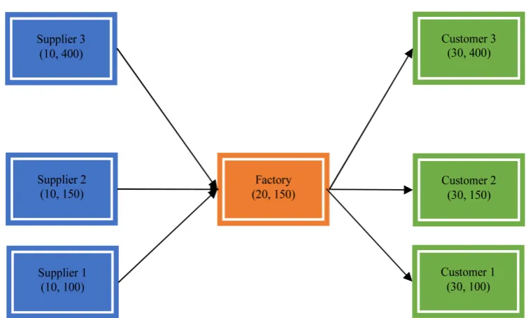
The system consists of three approved suppliers that serve the factory to serve three customers/distributors as shown in Figure 1.
2. Model Assumptions and Limitations
The following assumptions are considered: • The model has multi-objectives.
• Overall Service Level (OSL) is assumed as the ratio of the total weights deli-vered to the total weights required for all customers in all periods.
• Initial and ending inventory are assumed for all products.
• Costs parameters (fixed costs, material costs, manufacturing costs, non-utilized capacity costs, shortage costs, transportation costs, and inventory holding costs) are known for each location, each product at each period.
• All facilities have limited capacity for each period.
3. Model Formulation
The model involves the following sets, parameters and variables: Sets:
N: number of goals.
S: potential number of suppliers, indexed by s. C: potential number of customers, indexed by c. T: number of periods, indexed by t.
P: number of products, indexed by p. Parameters:
[image:3.595.162.540.487.714.2]Ff: fixed cost of the factory,
DEMANDcpt: demand of customer c from product p in period t, IIfp: Initial inventory of product p in the factory store,
FIfp: Final inventory of product p in the factory store, Ppct: unit price of product p at customer c in period t, Wp: product weight,
MHp: manufacturing hours for product p, Dsf: distance between supplier s and the factory, Dfc: distance between the factory and customer c, CAPst: capacity of supplier s in period t (kg),
CAPMft: capacity of the factory raw material store in period t, CAPHft: capacity in manufacturing hours of the factory in period t, CAPFSft: storing capacity of the factory in period t,
MatCost: material cost per unit supplied by supplier s in period t, MCft: manufacturing cost per hour for factory in period t, MHp: Manufacturing hours for product p,
NUCCf: non-utilized manufacturing capacity cost per hour of the factory, SCPUp: shortage cost per unit per period,
HC: holding cost per unit weight per period at the factory store, Bs: batch size from supplier s,
Bfp: batch size from the factory for product p, TC: transportation cost per unit per kilometer, Type: Type of goal objectives; percent or absolute, Sense: Sense of goal objectives; max or min. Decision Variables:
Ls: binary variable equal to 1 if a supplier s is contracted and equal to 0 other-wise,
Lis: binary variable equal to 1 if a transportation link is activated between supplier s and the factory,
Lic: binary variable equal to 1 if a transportation link is activated between the factory and customer c,
Qsft: number of batches transported from supplier s to the factory in period t, Qfccpt: number of batches transported from the factory to customer c for product p in period t,
Iffpt: number of batches transported from the factory to its store for product p in period t,
Ifccpt: number of batches transported from store of the factory to customer c for product p in period t,
Rfpt: residual inventory of the period t at the store of the factory for product p,
CSLc: Customer Service Level of customer c.
3.1. Objective Functions
while the third one is to maximize the Overall Service Levels of all customers. 1) Profit Objective
The Profit is calculated by subtracting the total cost from total revenue given in Equation (1).
(
)
Total Revenue cpt cpt p pct
c C p P t T
Qfc Ifc Bf P
∈ ∈ ∈
=
∑ ∑ ∑
+ (1)2) Total Cost Objective
The total cost is the summation of fixed, material, manufacturing, non-utilized capacity, shortage, transportation, and inventory holding costs calculated as shown in Equations (3) to (9).
3) Overall Service Level Objective
The Overall Service Level is the summation of the Customer Service Levels of all customers that calculated by Equation (2).
(
)
* * *c cpt cpt p p cpt p
p P t T p P t T
CSL Qfc Ifc Bf W DEMAND W
∈ ∈ ∈ ∈
=
∑ ∑
+∑ ∑
(2)3.2. Total Cost Elements
Total cost = fixed cost + material costs + manufacturing costs + non-utilized ca-pacity costs + shortage costs + transportation costs + inventory holding costs.
The cost elements of the total cost are calculated using Equations (3) to (9). 1) Fixed Cost
Fixed costs=Ff (3)
2) Material cost
1
Material cost sft s st p p s
s S t T p P
p p sT
p P
Q B MatCost IIf W MatCost
FIf W MatCost
∈ ∈ ∈
∈
= +
−
∑∑
∑
∑
(4)3) Manufacturing cost
1
Manufacturing cost fcpt p p t pt p p t
c C p P t T p P t T
p p p p T
p P p P
Q Bf MH Mc Iff Bf MH Mc
IIf MH Mc FIf MH Mc
∈ ∈ ∈ ∈ ∈
∈ ∈
= +
+ −
∑ ∑ ∑
∑ ∑
∑
∑
(5)4) Non-Utilized capacity cost (for the factory)
(
)
(
)
(
)
Non-Utilized capacity cost
ft f fcpt p p pt p p
t T p P c C p P
CAPH L Q Bf MH Iff Bf MH NUCCf
∈ ∈ ∈ ∈
= − −
∑
∑ ∑
∑
(6)5) Shortage cost (for customers)
(
)
1 1
Shortage cost
t t
cpt fcpt cpt p p
p P c C t T
DEMAND Q Ifc Bf SCPU
∈ ∈ ∈
= − +
∑ ∑ ∑ ∑
∑
(7)6) Transportation costs
(
)
Transportation cost sft s sf fcpt cpt p p fc
t T p P p P t T c C
Q B TcD Q Ifc Bf W TcD
∈ ∈ ∈ ∈ ∈
=
∑ ∑
+∑ ∑ ∑
+ (8)1
1 Inventory holding costs
T
pt p p pt p p
p P p P t
IIf Bf W HC Rf Bf W HC −
∈ ∈ =
=
∑
+∑ ∑
(9)3.3. Constraints
3.3.1. Balance Constraints
,
t s cpt p p pt p p
s S s S c C p P
Qsf B Qfc Bf W Iff Bf W t T
∈ ∈ ∈ ∈
= + ∀ ∈
∑
∑∑ ∑
(10)1 1 1 ,
p p p p fp cp p
c C
Iff Bf IIf Rf B Ifc Bf p P ∈
+ = +
∑
∀ ∈ (11)( )1 , 2 ,
pt p p t p pt p cpt p
c C
Iff Bf Rf − Bf Rf Bf Ifc Bf t T p P ∈
+ = +
∑
∀ ∈ → ∀ ∈ (12)(
)
( )( ) ( )
(
)
1 1
1 1 , , ,
cpt cpt p cpt cp t
t
p cp t cp t d D
Qfc Ifc Bf DEMAND DEMAND
Qfc Ifc Bf t T c C p P
− → − − ∈ + ≤ + − + ∀ ∈ ∀ ∈ ∀ ∈
∑
∑
(13),
pT p p
Rf Bf =FIf ∀ ∈p P (14) Constraint (10) ensures that the quantity of material entering to the factory from all suppliers equals the sum of the output to its store and customers.
Constraints (11)-(13) ensure that the sum of the flow entering to factory store and the residual inventory from the previous period is equal to the sum of the output to each customer and the residual inventory of the existing period for each product.
Constraint (14) ensures that the sum of the flow entering to each customer does not exceed the sum of the existing period demand and the previously accu-mulated shortages for each product.
3.3.2. Capacity Constraints
, ,
t s st s
Qsf B ≤CAP L ∀ ∈ ∀ ∈t T s S (15)
,
t s t f
s S
Qsf B CAPMf L t T ∈
≤ ∀ ∈
∑
(16),
cpt p pt p p t f
c C p P p P
Qfc Bf Iff Bf MH CAPHf L t T
∈ ∈ ∈
+ ≤ ∀ ∈
∑ ∑
∑
(17),
pt p p t f
p P
Rf Bf W CAPFS L t T
∈
≤ ∀ ∈
∑
(18)Constraint (15) ensures that the flow exiting from each supplier to the factory does not exceed the supplier capacity at each period.
Constraint (16) ensures that the sum of the material flow entering to the facto-ry from all suppliers does not exceed the factofacto-ry capacity of material at each pe-riod.
Constraint (17) ensures that the sum of manufacturing hours for all products manufactured in the factory to be delivered to its store and all customers does not exceed the manufacturing capacity hours of it at each period.
4. Model Verification
4.1. Model Inputs
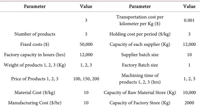
An example is assumed to verify the efficacy and efficiency of the model. The demands of all customers for all products in six periods are 550, 850, 450, 750, 350 and 850 units respectively. The beginning inventories of the three products are 50, 100, and 150 units with a total weight of 700 Kg (50 × 1 + 100 × 2 + 150 × 3) and the required ending inventories are 100, 150, and 200 respectively with a total weight of 1000 Kg (100 × 1 + 150 × 2 + 200 × 3). Other parameters are con-sidered as showing in Table 1.
The first objective is to maximize the profit; the second objective is to minimize the total cost, while the third objective is to maximize the OSL without any al-lowable deviation for the objectives to simplify the model verification process.
4.2. Model Outputs and Discussion
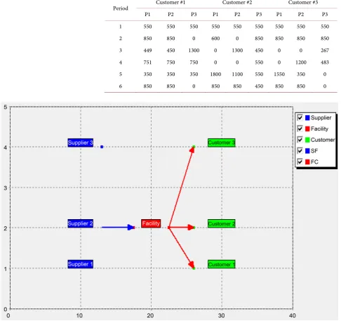
The optimal factory network is shown in Figure 2. The factory shall take its ma-terial only from the second supplier to reduce the transportation cost where it is the nearest one. The quantities of products delivered to each customer in all of the six periods are shown in Table 2.
The factory shall serve the three customers but with different service levels which are shown in Figure 3. It can be noticed that the CSL of the second cus-tomer is the highest one because of its closeness to the factory that maximizes the profit (first objective).
The optimal values of the three objectives; Profit, total cost, and Overall Ser-vice Level are $3,053,853.8, $1,496,146.2, and 87.28%.
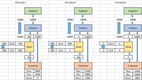
[image:7.595.209.538.554.732.2]The model results of flow are verified through this example as shown in Fig-ure 4 and Figure 5. Figure 4 represents the flow balancing of weights during the first three periods since it is noticed that, during the first period the factory re-ceived 10 tons of material and supply 9700 kg directly to the customer to satisfy some of their demand and store 300 in its store which had an initial inventory of
Table 1. Verification model parameters.
Parameter Value Parameter Value
3 Transportation cost per kilometer per Kg ($) 0.001
Number of products 3 Holding cost per period ($/kg) 3 Fixed costs ($) 50,000 Capacity of each supplier (Kg) 12,000 Factory capacity in hours (hrs) 12,000 Supplier batch size 10 Weight of products 1, 2, 3 (Kg) 1, 2, 3 Factory Batch size 1
Price of Products 1, 2, 3 100, 150, 200 products 1, 2, 3 (hrs) Machining time of 1, 2, 3
Table 2. Quantities of products delivered to each customer in all of the six periods.
Period Customer #1 Customer #2 Customer #3 P1 P2 P3 P1 P2 P3 P1 P2 P3 1 550 550 550 550 550 550 550 550 550 2 850 850 0 600 0 850 850 850 850 3 449 450 1300 0 1300 450 0 0 267 4 751 750 750 0 0 550 0 1200 483 5 350 350 350 1800 1100 550 1550 350 0 6 850 850 0 850 850 450 850 850 0
Figure 2. The optimal factory network.
700 kg to send 200 kg from its initial inventory (FIFO) to the customers to satis-fy the remaining demand without shortage. A shortage of 4500 kg can be noticed in the second where the demand of the second period requires 15,300 kg of raw material which exceeds the factory capacity of the material of 10,000 kg and stored quantity of 800 kg. This shortage increases the net accumulated demand of the third period to 12,600 which lead to reduce the accumulated shortage to 2600 kg.
Figure 3. The resulted CSL of the customers.
Figure 4. Flow balancing of weights during the first three periods.
enforced to fulfill the ending inventory of 1000 kg which increases the total shortage of the three customers to 8700 kg. So, the overall service level is lowered by (8700/68,400) × 100 = 12.72% to be 87.28% as mentioned above.
5. Computational Results and Analysis
Through this section, the effect of the deviation percentages on the different ob-jectives is discussed. The three obob-jectives percent deviation taken in this study are 0, 5, 10, and 15 that gave a combination of 64 for different values of the al-lowable percent deviation for each objective. The results of the 64 cases are pre-sented in Table 3 which is divided into three parts for the values of each objec-tive for each case. Through all cases, it may be noticed that the percent deviation of the last objective (OSL in these cases) almost have no effect on the results of
88.82% 94.74%
78.29%
C 1 C 2 C 3
CSL
10000 10000 10000
10000 300 9700 10000 0 10000 10000 0 10000
1000 Start 700 800 Start 800 0 Start 0
1000 End 800 800 End 0 0 End 0
200 800 0
Dem. 9900 Req. 15300 Req. 12600
Rec. 9900 Rec. 10800 Rec. 10000
Short. 0 Short. 4500 Short. 2600
Period # 1 Period # 2 Period # 3
Customer
Supplier
10000
Factory
Store
Customer Factory
Store
Supplier Supplier
10000 10000
Factory
[image:9.595.60.538.253.522.2]Figure 5. Flow balancing of weights during the last three periods.
Table 3. The resulted optimal objectives values of the 64 cases.
Profit Values
Profit Dev. % OSL Dev. % Total Cost Deviation %
0% 5% 10% 15%
0 0 - 15 3,053,854 3,053,854 3,053,854 3,053,854 5 0 - 15 2,901,186 3,013,381 2,911,892 2,916,762 10 0 - 15 2,748,476 3,009,926 2,965,211 2,856,811 15 0 - 15 2,595,779 3,005,124 2,990,731 2,856,811
Total Cost Values
Profit Dev. % OSL Dev. % Total Cost Deviation %
0% 5% 10% 15%
0 0 - 15 1,496,146 1,496,146 1,496,146 1,496,146 5 0 - 15 1,466,414 1,536,619 1,595,608 1,595,608 10 0 - 15 1,440,774 1,511,724 1,584,789 1,592,889 15 0 - 15 1,417,521 1,488,376 1,559,269 1,592,889
OSL Values
Profit Dev. % OSL Dev. % Total Cost Deviation %
0% 5% 10% 15%
0 0 - 15 87.3 87.3 87.3 87.3
5 0 - 15 83.6 87.3 87.3 87.3
10 0 - 15 80.0 87.3 87.3 87.3
15 0 - 15 76.9 87.0 87.3 87.3
10000 10000 10000
10000 0 10000 10000 0 10000 10000 1000 9000
0 Start 0 0 Start 0 1000 Start 0
0 End 0 0 End 0 1000 End 1000
0 0 0
Req. 16100 Req. 12400 Req. 17700
Rec. 10000 Rec. 10000 Rec. 9000
Short. 6100 Short. 2400 Short. 8700
10000
Factory Factory
Customer Customer
Supplier
10000
Period # 4 Period # 5 Period # 6
Factory
Store Store Store
Customer Supplier
10000
[image:10.595.209.538.377.737.2]the model. So, the effect of other deviation on the value of the objectives is dis-cussed and analyzed.
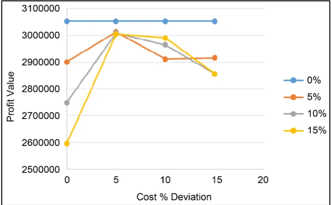
[image:11.595.206.538.235.440.2]The effect of the cost percent deviation and profit percent deviation on the profit (The first objective) values is depicted in Figure 6. It is clear to notice that, at zero profit percent deviation, the profit value does not change by changing the cost percent deviation which is logic where there is no possibility to reduce the achieved profit to get more optimal values for the total cost. Increasing of the profit percent deviation reduces its values.
[image:11.595.207.537.485.702.2]Figure 7 represents the effect of the cost percent deviation and profit percent deviation on the total cost (The second objective). It can be noticed that, at zero
Figure 6. The effect of the cost percent deviation and profit percent deviation on the profit values.
Figure 7. The effect of the cost percent deviation and profit percent deviation on the total cost values.
1400000 1420000 1440000 1460000 1480000 1500000 1520000 1540000 1560000 1580000 1600000 1620000
0 5 10 15 20
Tot
al
C
os
t V
al
ue
Cost % Deviation
profit percent deviation, the total cost value does not change by changing the cost percent deviation which is logic where there is no possibility to get more optimal values by reducing the achieved profit. Increasing of the profit percent deviation decreases the total cost values while increasing of the total cost percent deviation increases the total cost values as shown in Figure 7 and increases the profit values as shown in Figure 6.
Figure 8 represents the effect the cost percent deviation and profit percent deviation on the OSL (The third objective). It can be noticed that, at zero profit percent deviation, the OSL value does not change by changing the cost percent deviation which is logic for the same reasons mentioned before. Increasing of the profit percent deviation decreases the OSL values while increasing of the total cost percent deviation increases the OSL.
6. Conclusions and Future Recommendations
The developed model efficacy and efficiency are verified through a general ex-ample representing a general case of a factory with assumed initial and ending inventory values for all products. The model is a general one and may be customized easily to many real cases. The behaviour of the model is analysed and the logicality of its results are proved.
The developed model is capable of optimizing production planning for multi- objectives ordered according to their priorities to the planner.
The model is capable to solve larger problems as compared to the problems considered in the present work.
Figure 8. The effect of the cost percent deviation and profit percent deviation on the OSL values.
76.0 78.0 80.0 82.0 84.0 86.0 88.0
0 5 10 15 20
O
SL
Va
lu
e
Cost % Deviation
The performance of the factory is affected by the ordering of its objectives in addition to the allowable deviation of them.
The developed model dealt with deterministic demand and it is recommended to tackle the stochastic one. Also, it is recommended to solve the same problem using different methods and comparing the results to clarify the advantages and disadvantages of each one.
References
[1] http://www.fico.com/en/node/8140?file=5097
[2] Guillén, G., Mele, F.D., Bagajewicz, M.J., Espuña, A. and Puigjaner, L. (2005) Multi Objective Supply Chain Design under Uncertainty. Chemical Engineering Science, 60, 1535-1553.
[3] Altiparmak, F., Gen, M., Lin, L. and Paksoy, T. (2006) A Genetic Algorithm Ap-proach for Multi-Objective Optimization of Supply Chain Networks. Computers and Industrial Engineering, 51, 196-215.
[4] Liu, S. and Papageorgiou, L.G. (2013) Multi Objective Optimisation of Production, Distribution and Capacity Planning of Global Supply Chains in the Process Indus-try. Omega, 41, 369-382.
[5] Sawik, T. (2007) A Lexicographic Approach to Bi-Objective Scheduling of Single Period Orders in Make-to-Order Manufacturing. European Journal of Operational Research, 180, 1060-1075.
[6] Mavrotas, G. (2009) Effective Implementation of the E-Constraint Method in Mul-ti-Objective Mathematical Programming Problems. Applied Mathematics and Com-putation, 213, 455-465.
[7] Pishvaee, M.S., Razmi, J. and Torabi, S.A. (2012) Robust Possibilistic Programming for Socially Responsible Supply Chain Network Design: A New Approach. Fuzzy Sets and Systems, 206, 1-20.
[8] Vieira, G.E. and Favaretto, F. (2006) A New and Practical Heuristic for Master Production Scheduling Creation. International Journal of Production Research, 44, 18-19, 3607-3625.https://doi.org/10.1080/00207540600818187
[9] Chern, C.C. and Hsieh, J.S. (2007) A Heuristic Algorithm for Master Planning That Satisfies Multiple Objectives. Computers & Operations Research, 34, 3491-3513. [10] Wu, Z., Zhang, C. and Zhu, X. (2012) An Ant Colony Algorithm for Master
Pro-duction Scheduling Optimization. Proceedings of the 2012 IEEE 16th International Conference on Computer Supported Cooperative Work in Design(CSCWD), 23-25 May 2012, 775-779.
[11] Soares, M.M. and Vieira, G.E. (2009) A New Multi-Objective Optimization Method for Master Production Scheduling Problems Based on Genetic Algorithm. Interna-tional Journal Advanced Manufacturing Technology, 41, 549-567.
https://doi.org/10.1007/s00170-008-1481-x
[12] Zapfel, G., Braune, R. and Bogl, M. (2010) Metaheuristic Search Concepts: A Tu-torial with Applications to Production and Logistics. Springer, Heidelberg Dor-drecht London New York.
Submit or recommend next manuscript to SCIRP and we will provide best service for you:
Accepting pre-submission inquiries through Email, Facebook, LinkedIn, Twitter, etc. A wide selection of journals (inclusive of 9 subjects, more than 200 journals)
Providing 24-hour high-quality service User-friendly online submission system Fair and swift peer-review system
Efficient typesetting and proofreading procedure
Display of the result of downloads and visits, as well as the number of cited articles Maximum dissemination of your research work