An Improved Algorithm Based on the GVF-Snake for
Effective Concavity Edge Detection
*
Mengmeng Zhang, Qianqian Li, Lei Li, Peirui Bai
College of Information and Electrical Engineering, Shandong University of Science and Technology, Qingdao, China. Email: [email protected]
Received January 18th, 2013; revised February 12th, 2013; accepted February 21st, 2013
Copyright © 2013 Mengmeng Zhang et al. This is an open access article distributed under the Creative Commons Attribution Li-cense, which permits unrestricted use, distribution, and reproduction in any medium, provided the original work is properly cited.
ABSTRACT
Image segmentation is an important research area in Computer Vision and the GVF-snake is an effective segmentation algorithm presented in recent years. Traditional GVF-snake algorithm has a large capture range and can deal with boundary concavities. However, when interesting object has deep concavities, traditional GVF-snake algorithm can’t converge to true boundaries exactly. In this paper, a novel improved scheme was proposed based on the GVF-snake. The central idea is introduce dynamic balloon force and tangential force to strengthen the static GVF force. Experimen- tal results of synthetic image and real image all demonstrated that the improved algorithm can capture boundary con- cavities better and detect complex edges more accurately.
Keywords: Image Segmentation; the GVF-Snake; Boundary Concavities; Balloon Force; Tangential Force
1. Introduction
Active contours model, a tracking method using active curves or surfaces, has been proposed in recent years. It can integrate edge and region information and has been widely used in image segmentation field. The most widely used active contours model include snakes and level set [1]. Snakes were firstly introduced by Kass and its basic idea is to make the initial closed curve (i.e. a sequence of discrete points) converge to the desired edge by mini- mizing the energy functional [2]. However, the classical snakes have three main disadvantages. The first is topo- logical structure of the curves can’t change flexibly. Secondly, the initial curve only converges steadily when it lies close to the desired edge. Thirdly, it is not easy to handle boundary concavities. To solve the first problem, McInerney et al. proposed T-snake which not only main-tains strong interactivity of the classical snakes but also improves the changing ability of topological structure [3]. Sun et al. introduced adaptive filters to T-snake so that it can deal with several interlaced objects [4]. Zagorchev et al. proposed R-snake based on rotating Gaussian curve [5]. R-snake is capable of changing the curve’s rigidity,
so object’s shape could be reconstructed smoothly. To the second problem, Cohen et al. has proposed the bal- loon snake [6] and the distance snake [7]. Both of them increase the capture range of external force field and make the placing of initial curve easy. To the third prob- lem, Xu et al. has introduced the GVF-snake which not only enlarges capture range but also can deal with bound- ary concavities [8]. Luo et al. presented an additional balloon force to the GVF-snake to prevent the active curve from trapping into local minima [9]. Zhu proposed a nonlinear filtering on GVF force field to further enlarge capture range [10]. Although the GVF-snake has large capture range and considerable ability to handle bound- ary concavities, it is difficult to realize accurate segmen- tation when detecting complex shape object with deep concavities. Accordingly, we introduce dynamic balloon force and tangential force to strengthen the static GVF force, and it is found that the capability of capturing concave edges enhanced effectively.
2. Principles and Methods
2.1. The GVF-Snake
*Supported by Shandong Province Natural Science Foundation
(ZR2009CMO32), Project of Shandong Province Higher Educational Science and Technology Program (J09LG19) and Research Project of SUST “Spring Bud” (NO2009AZZ153).
1 2
0 1
d
2 ext
E
X s X s E X s s (1) where X s
and X s
denote the first and second derivatives of X(s) with respect to s, α and β are weight- ing parameters that control smoothness and tautness of the snake respectively. External energy Eext
X s
is used for moving the snake towards edges or other inter- esting features. To minimize the energy function, the energy Equation (1) can deduce to the force-balance equation using the calculus of variations, i.e. the Euler equation is as follows:
ext 0X s X s E
(2) The former two terms represent the internal force Fint
and the negative gradient of a potential function repre- sents the external force Fext. When the internal force and
the external force reach their balance, the energy func- tional converges to its minima.
The main difference between the GVF-snake and the classical snake model lies on the different external forces. For the GVF-snake, the external force Fext is replaced by
the gradient vector flowV x y
,
u x y v x y
,
, ,
, where V x y
, is achieved by minimizing the following energy function:
2 2 2 2
2 2d d
x y y y
u u u v f V f x y
(3) where, f denotes the gradient of edge map and μ is a weighting parameter. μ should choose a large value when the image is noisy. When f is small, the energy is dominated by the first partial derivatives, so it is a slowly-varying field. When f is large, the second term dominates the energy and energy minima can be achieved by setting V f .In order to minimize the energy of Equation (3), it must satisfy the following Euler equation:
2 2 0
x x y
u u f f f
2 (4)
2 2 0
y x y
v v f f f
2 (5) where is the Laplacian operator. In homogeneous regions, both fx and fy are zero. In this case, u and v are
dominated by Laplacian equation. Within the boundary regions, the snake mainly performs a “filling in” property. We can get from Equation (3) and set X as func- tion of time X(s,t), the dynamic equation is obtained as follows:
2
( , ) V x y
,
,
, 1t
X s t X s t X s t V (6) where V represents static GVF force, 1 is a weighting parameter. When
,t
X s t is equal to zero, stable solu- tion of the GVF-snake is achieved.
2.2. The Improved GVF-Snake
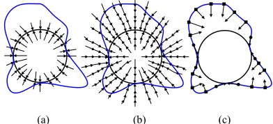
The GVF-snake can’t converge to deep boundary con- cavities accurately, so we propose to design dynamic balloon force and tangential force to strengthen the GVF force to improve the capture ability of desired edges. To demonstrate the effect of the additional forces, Figure 1
shows external forces field of the traditional snake, the GVF-snake and the improved GVF-snake, respectively.
In Figure 1, the circle denotes the desired edge and the
arrow denotes the force direction. The curve denotes the active contour and the point on the curve denotes control point. It can be seen that force field of the traditional snake is narrow and very close to the desired edge.
The force field of the GVF-snake showed in Figure 1(b) can effectively enlarge capture range throughout the
whole image. Therefore, the GVF-snake can overcome the initialization problem related to the traditional snake. The improved GVF-snake is considered to combine the static GVF force field and two kinds of dynamic forces which are showed in Figure 1(c). The balloon force is
used to increase capture range and converging speed of snake, and the tangential force is used to make the snake converge to boundary concavities better.
It is noted that the proposed balloon force and tangen- tial force can change their affect area adaptively. The value of each control point is replaced by the average value of its nine surrounding pixels. It indicates that the control point denoted by squared point is far away from the desired edge when the averaged value is smaller than the given threshold T. In this case, the balloon force pulls snake towards the edge. When the averaged value is big- ger than T, it means this control point is close to the edges. In this case, the tangential force is used to ap- proach the edge. At the same time, it can prevent the snake from breaking through weak edges.
If T is choose too large, the balloon force is still af- fecting nearby the desired edge while the capture range of the tangential force becomes smaller, and it is difficult to avoid boundary leakage. If T is too small, only the tangential force is affected near to the edges, and the snake is hard to converge to deep concave boundary. So the value of threshold T is advised to 0.2 ~ 0.5.
[image:2.595.325.521.608.697.2](a) (b) (c)
The force balance equation of the improved GVF- snake can be expressed as follows:
g n q 0
int ext ext ext
F F F F (7) where Fint represents the internal force, Fext g represents
the GVF force, n ext
F represents the balloon force, q ext
F represents the tangential force. They are defined respec- tively as follows:
1 2 3 , , , g ext n ext q extF V x y
F sign n N x y F sign q Q x y
(8)
where 1, 2 and 3 are weighting parameters of the GVF force, the balloon force and the tangential force respectively. N(x,y) represents outward unit normal vec- tor. When the active contour lies inward the desired edge,
sign(n) > 0 and the active contour inflates. When the ac- tive contour lies outward the desired edge, sign(n) < 0 and the active contour deflates.
,Q x y represents the unit tangential force. Sign(q) is obtained by computing the inner product of V x
,y and Q x y
, :
,
,
,
,
coq V x y Q x y V x y Q x y s (9) where θ is the angle between V x y
, and Q x y
, . Ifθ lies in
π 2,3π 2 ,
and it indicates the two vectors are inconsistent. It is necessary to negate the tan- gential vector to ensure the snake converging normally. If θ lies in0
q
0,π 2 or
3π 2, 2π
, q . It indicates that the two vectors are consistent and the direction of tangential vector needn’t change. Accordingly,0
q ext
F can be expressed as follows:
3
3
π 3π
, 0 or π
2 2
π 3π
,
2 2
q ext
Q x y F
Q x y
2
, (10)then, Equation (7) can be expressed as follows:
1 2 3 , , 0 intF V x y sign n N x y
sign q Q x y
(11)
Therefore, the improved GVF-snake is expressed as follows:
,
,
, 1 2 3t
X s t X s t X s t V N Q
t t t t (12)Equation (12) can be quantized and expressed using matrix formation as follows:
1 1 1 2 3 1 1 1 2 3 , , , , , ,t t x
x t t x t t
t t y
y t t y t t
x A I x V x y
N x y Q x y
y A I y V x y
N x y Q x y
(13)
where γ is temporal step-size.
3. Experiments and Results
Experiments were designed to compare segmentation performance of the GVF-snake and the improved GVF- snake. All computation is done under the environment of computer X42J (ASUS Inc.). CPU is 2.00 GHz and RAM is 2 GB. Operation system is Windows XP-SP3 and the programming tool is MATLAB 7.0.
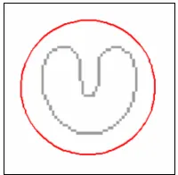
Figure 2 shows a U-shape test image U64.pgm along
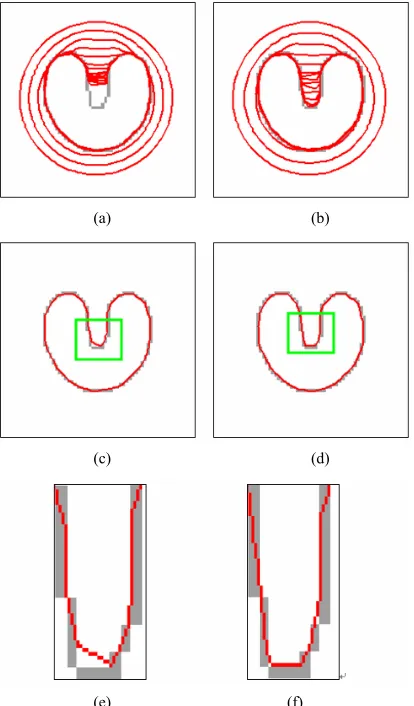
with an initial circle curve. Image size is 64 × 64. Figure 3(a) shows segmentation procedure of the GVF-snake
with maximum iteration number set as 80. Figure 3(b)
shows similar segmentation procedure of the improved GVF-snake with same computing parameters as in Fi- gure 3(a)i.e. α = 0.05, β = 0, γ = 1, μ = 0.2, κ1 = 0.6, κ2 =
−0.15, κ3 = 0.2, T = 0.3. It can be seen that the improved GVF-snake converge towards the boundary concavities faster than the GVF-snake with 80 iterations. The reason is that the GVF-snake is driven only by the GVF force, while the improved GVF-snake is driven by a combina-
tion of balloon force, tangential force and GVF force.
Figures 3(c) and (d) show the segmentation results of the
GVF-snake and the improved GVF-snake at 125 itera- tions respectively. For convenient comparison, the boun- dary concavities section denoted by the rectangle in Fi- gures 3(c) and (d) are zoomed in as shown in Figures 3(e) and (f). It can be seen clearly that the former snake
can’t converge to the deep boundary concavity well, while the latter snake converges to the deep boundary concavity more exactly. So, the improved GVF-snake proposed in this paper not only converges to boundary concavity faster than the GVF-snake but also its capture capacity of deep concave edges is also better than the classical GVF-snake.
Figure 4 shows a left clavicle image clavicle.bmp
along with an initial manual curve. Image size is 269 × 210. Figures 5(a) and (b) show the results of 200 itera-
tions of the GVF-snake and the improved GVF-snake respectively. The computing parameters are same i.e. α = 0.05, β = 0, γ = 1, μ = 0.2, κ1 = 0.6, κ2 = 0.25, κ3 = 0.5, T = 0.3. It can be seen from Figure 5(a) that the GVF-snake
didn’t converge to the thin concave boundary exactly at
[image:3.595.373.473.619.717.2](a) (b)
(c) (d)
[image:4.595.70.277.86.439.2](e) (f)
Figure 3. Segmentation results of U-shape image of the GVF-snake and the improved GVF-snake. ((a) 80 iterations of the GVF-snake; (b) 80 iterations of the improved GVF- snake; (c) 125 iterations of the GVF-snake; (d) 125 itera-tions of the improved GVF-snake; (e), (f) the zoom in view-point of boundary concavities section denoted by the rec-tangle as shown in Figures 3(c) and (d)).
Figure 4. Left clavicle image along with an initial manual curve.
three positions denoted by arrows. However, the seg-mentation result in Figure 5(b) indicates that obvious
[image:4.595.307.535.86.186.2] [image:4.595.307.539.285.370.2]improvement is achieved by the improved GVF-snake.
Table 1 lists a quantitative performance comparison of
the GVF-snake and the improved GVF-snake. Quantita-
(a) (b)
Figure 5. Segmentation results of left clavicle image of the GVF-snake and the improved GVF-snake. ((a) 200 itera-tions of the GVF-snake; (b) 200 iteraitera-tions of the improved GVF-snake).
Table 1. Quantitative comparison of segmentation per-formance between the GVF-snake and the improved GVF- snake.
MN/pixels T/s
Quantitative parameter Segmentation method
U-shape image
left clavicle image
U-shape image
left clavicle image
The GVF-snake 0.4528 4.9346 15.0160 33.2190 The improved
GVF-snake 0.4402 4.9093 15.0470 33.5940 tive parameters are MN (the mean error between active contour and the desired boundary with unit of pixel number) and T (the computation time with unit of sec-ond). The MN and T of U-shape image and left clavicle image using the GVF-snake and the improved GVF- snake are listed. As indicated in Table 1, the
computa-tion time of the improved GVF-snake is slightly longer than the GVF-snake, but its MN is much smaller than that of the GVF-snake. It means that the improved GVF- snake can achieve exciting segmentation accuracy than the GVF-snake at the little cost of computation time.
4. Conclusion
[image:4.595.106.239.532.635.2]REFERENCES
[1] L. He, Z. G. Peng, B. Everding, et al., “A Comparative Study of Deformable Contour Methods on Medical Image Segmentation,” Image and Vision Computing, Vol. 26, No. 2, 2008, pp. 141-163.
doi:10.1016/j.imavis.2007.07.010
[2] M. Kass, A. Witkin and D. Terzopoulos, “Snakes: Active Contour Models,” International Journal of Computer Vi-sion, Vol. 22, No. 1, 1988, pp. 321-331.
[3] T. McInerney and D. Terzopoulos, “T-Snakes: Topology Adaptive Snakes,” Medical Image Analysis, Vol. 4, No. 2, 2000, pp. 73-91. doi:10.1016/S1361-8415(00)00008-6 [4] F. R. Sun, Z. Liu, Y. L. Li, et al., “Improved T-Snake
Model Based Edge Detection of the Coronary Arterial Walls in Intravascular Ultrasound Images,” The 3rd In-ternational Conference on Bioinformatics and Biomedical Engineering (iCBBE2009), Beijing, June 2009, pp. 1-4. [5] L. Zagorchev, A. Goshtasby and M. Satter, “R-Snakes,”
Image and Vision Computing, Vol. 25, No. 6, 2007, pp. 945-959. doi:10.1016/j.imavis.2006.07.008
[6] L. D. Cohen, “On Active Contour Models and Balloons,” CVGIP: Image Understand, Vol. 53, No. 2, 1991, pp. 211- 218.
[7] L. D. Cohen and I. Cohen, “Finite-Element Methods for Active Contour Models and Balloons for 2D and 3D Im- ages,” IEEE Transaction on Pattern Analysis and Ma- chine Intelligence, Vol. 15, No. 11, 1993, pp. 1131-1147. doi:10.1109/34.244675
[8] C. Y. Xu and J. L. Prince, “Snakes, Shapes, and Gradient Vector Flow,” IEEE Transaction on Image Processing, Vol. 7, No. 3, 1998, pp. 359-369. doi:10.1109/83.661186 [9] S. Luo and R. Li, “A New Deformable Model Using
Dy-namic Gradient Vector Flow and Adaptive Balloon Forces,” APRS Workshop on Digital Image Computing, Brisbane, 2003, pp. 9-14.
[10] X. J. Zhu, P. F. Zhang, J. H. Shao, et al., “A Snake-Based Method for Segmentation of Intravascular Ultrasound Images and Its in Vivo Validation,” Ultrasonics, Vol. 51, No. 2, 2011, pp. 181-189.