The Riemannian Structure of the Three-Parameter
Gamma Distribution
William W. S. Chen1, Samuel Kotz2
1Department of Statistics, The George Washington University, Washington DC, USA
2Department of Engineering Management and Systems Engineering, The George Washington University, Washington DC, USA Email: [email protected]
Received October 24, 2012; revised January 11, 2013; accepted January 18, 2013
ABSTRACT
In this paper, we will utilize the results already known in differential geometry and provide an intuitive understanding of the Gamma Distribution. This approach leads to the definition of new concepts to provide new results of statistical importance. These new results could explain Chen [1-3] experienced difficulty when he attempts to simulate the sam- pling distribution and power function of Cox’s [4,5] test statistics of separate families of hypotheses. It may also help simplify and clarify some known statistical proofs or results. These results may be of particular interest to mathematical physicists. In general, it has been shown that the parameter space is not of constant curvature. In addition, we calculated some invariant quantities, such as Sectional curvature, Ricci curvature, mean curvature and scalar curvature.
Keywords: Mean Curvature; Gamma Distribution; Ricci Curvature; Riemannian Geometry; Scalar Curvature; Sectional Curvature
1. Introduction
This paper will cover the study of the geometrical struc- ture of the parameter space of the three parameter Gamma distribution. Rao [6] was one of the first to propose the differential-geometrical approach to parameter spaces, by introducing a Riemannian metric in terms of the Fisher Information matrix. The major objective of this paper is to utilize the results already known in differential geo- metry and provide an intuitive understanding of the three parameter Gamma Distribution. This approach leads to the definition of new concepts, which provide new re- sults of statistical importance. These points will be clear in the concluding remark. Pioneer work in this direction was done by Efron [7], who introduced the notion of the so called “statistical curvature” of a one-parameter stati- stical model. Later, he showed that the statistical cur- vature is closely related to Fisher and Rao’s theory of second-order efficiency. Recently, there have been some new developments in this area. Mitchel A.F.S. [8] studies alpha-curvature tensor and alpha-geodesics of the elliptic distribution. Burbea and Rao [9] also study distances be- tween distributions more particularly the multinomial and the normal distributions. Skovgaard [10] defines and provides some details on the geometry of the multivariate normal manifold. Sato et al. [11] has listed all the possi-
ble sectional curvatures of the bivariate normal distribu- tion. Kass R.E. and Vos P.W. [12,13] gave an organized
and through summary in this area. In Section 2, we de- fined the fundamental Riemannian metric tensor and its inverse tensor. In Section 3.1, we define and derive the sectional curvature. In Section 3.2, the definition and ori- gin of the Ricci curvature tensors will be given and then used to find the mean curvatures of each direction and the scalar curvature of the parameter space. In Section 4, we list all nonzero Riemannian tensors for reference pur- poses. In the concluding remarks we tabulate the three sectional curvature and mean curvature versus a function of shaped parameter. Finally, we plot on the vertical axis of these tabulated seven functional values against its shape parameter as horizontal axes. In this way we could clearly see the validity of the function and the points where functions are undefined. It is helpful to use the “REDUCE Programming Language” [14] to perform the needed computation.
2. The Parameter Space and Riemannian
Metric
Let us consider a family of gamma distribution with ran- dom variables x, such that a distribution is specified by a
set of 3 real parameters
1, ,2 3
3 R
1, ,2 3
. Then we can construct an 3-dimensional space of distributions with a coordinate system . Let f x
, denote the probability density function of x specified byfunctions exist and smooth in the space. A maximal smooth structure may be introduced making the family a 3-dimensional smooth manifold. A family of densities having a locally 3-dimensional Euclidean topology to- gether with a maximal smooth structure will be called a 3-dimensional manifold of densities.
When the parameter space is in a higher dimension, a certain coordinate system, that specifies a point p on the n-dimensional manifold, by
1, , ,2 n
is considered.The squared distance between two neighboring points p
and p+dp,
1, , ,2 n
, , ,
d d
,
1 1 2 2 ndn
, can be represented bythe quadratic form g d dij i j, where gij is the compo-
nent of Fisher’s Information matrix defined by
2 2
ln , ln ,
ln ,
, , 1, 2, ,
ij
i j
ij
f x f x
g E
f x
E i j
n
(2.1)
where E denotes the expectation with respect to the dis-
tribution f x
, .If these quadratic form is a symmetric positive definite metric tensor then the surface is said to form a Rieman- nian manifold.
A random variable x has a Gamma distribution if its
probability density function is:
1; , , 1
exp .
,0 ,0 .
0 otherwise.
f x
x x
x
(2.3)
The distribution is known as the Type III of Pearson’s system. This distribution depends on three parameters
, and
. They are known as the location, scale and shape parameters. This distribution has widely been em- ployed as a model for distributions of life span, reaction time, and related phenomena. The three-parameter Gam- ma distribution has shapes similar to the Weibull, Log- normal, and Inverse Gaussian Distribution. Balakrishnan N. and Chen W. [15] will publish a handbook that tabu- lates the coefficients of “BLUP” of the estimable func- tion for the location and scalar parameters for some com- monly used for given shape parameters. A list of 130 references in Johnson and Kotz [16] is located at the end of Chapter 17, pp. 200-206. An updated revised version by Johnson, Kotz and Balakrishnan [17] listed more than 310 references at the end of Chapter 17, pp. 397-414.
These are the most complete resources for this distribu- tion. In both editions the authors have suggested that maximum likelihood of estimating equations (MLE) should not be used unless the shape parameter is greater than 2.5. A detailed discussion of this observation will be given at the concluding remarks.
Gamma distribution contains three parameters:
, ,
. In some coordinate systems we can consider a three-dimensional parameter space where one point can be represented by the number
, ,
. 1 , 2 and
To simplify our notation it would be convenient to reparameterize our parameters as
. or , ,
3 1 2 3
.
Using the definition of (2.1), we can derive our Rie- mannian Metric Tensor of the three-parameter Gamma distribution in the following form:
2 2
3 2
3 2 2
3
2 2
2
2 2
3
3 2 2
1 1 1
1 2
1
1 1
1
ij
G g
1
(2.4)
In Equation (2.4), the distribution property (2.3) re- stricts 20
,and
. It is also clear that when the shape pa- rameter equals 1 or 2, the Riemannian Metric Tensors
11, 13 31
g g g do not exist. In fact, when 31, the distribution in (2.3) reduces to an exponential distribu- tion. Additionally, when 32 or when closing on either from left side or right side of 2, the g11-Tensor will become infinitely large. The concluding remarks will discuss this case in detail. Due to the commonly known distributional property of gamma, that digamma functions are only undefined at negative integers and at zero, the shape parameter 3 must be a positive real value in order to guarentee the existence of g33.
In the three parameters gamma distribution we can show the determinant G is rank 3 and hence can form an
3-dimensional smooth manifold. However, if the location parameter is fixed then scalar and shape parameters can form a 2-dimensional smooth maniforld only. In (2.4), each element of the matrix does not involve the location parameter. Hence the rank of matrix is full rank after the location parameter is fixed. This means the 2-manifold formed by scale and shape parameters is not a geodesic submanifold of the 3-manifold.
Again, to simplify our notation, we will set the nu- merator of determinant G equal to Δ. Hence,
23 3
2 2
3 3 3 2 3 2 3 3 2
2 2
3 2 2 3 2
1
2
3 3 2 3 2 3
2 2 1 2 1 2
2 2
1 2 1 1
2 2
1 2 1 2 1
ij
G g
(2.5)
where the inverse
ijg of the Riemannian Metric Ten- sor
gij will satisfy the relation .ik k
ij j
g g The
Kronecker Symbol
i en hen ;
k
j k j k j
1 1
for e e, s 1 wh
xampl
, and 0 w
1 2
1, 0
point in M. The Gaussian Curvature at a point p on the
surface, geodesic at p, and tangent to a plane in the
tangent space at p is called the sectional curvature at
p,
. If
,
is any basis for the plane , wewould use the notation K
,
for the sectional cur- vature and define it as follows:.
3. Structure of the Parameter Space
,
i j k l ijkl
i j k l ik jl jk il
R k
g g g g
(3.1)
3.1. Sectional Curvature
This section will give some geometrical quantitative in- terpretations to the curvature tensor in n-dimensional
space. Let M be a Riemannian n-manifold and let p be a
In the case of the three-parameter Gamma Distribution, we can apply Formula (3.1) to find the sectional curva- ture in the following form:
3 2
3 3 3 3 3 3 3
3
2
3 3
3
3 3 3 3
3 3
2 2
2 5 8 4 7 2 4 1 2
2 2 1
1, 2 , 1,3 ,
4 2 4 1 2
4 9 2 3 4 1
2,3 ,
4 2
d d
where ln , .
d d
k k
k
x x x x
x x
(3.2)
3.2. Ricci Tensor and Related Curvatures If M is a two-dimensional space, it is clear that the
sectional curvature coincides with the Gaussian Curva- ture. If the sectional curvature at every point of a Rie- mannian n-Manifold M does not depend on the two-di-
mensional section passing through the point, then it is constant over the manifold. Such a Riemannian n-Mani- fold is said to be of constant curvature. The Equation (3.2) show that all three sectional curvatures are functions of the shape parameter. Clearly, they are not of constant curvature. The detailed discussion about the vertical or horizontal asymptotic lines of these functions are given at the concluding remarks (See Figure 1).
The four dimensional Riemannian Tensors are compli- cated, it would be better to construct simpler tensors that summarize some of the information contained in the cur- vature tensor. The most important of such tensors is the Ricci curvature tensor, or simply, the Ricci tensor. De- noted Ricci, which is the covariant 2-tensor field defined as the trace of the curvature endomorphism, on its first and last indices. The components of Ricci are usually denoted Rjk, so that .
il
jk ijkl
R g R For the space of a three-parameter Gamma Distribution, the components of the Ricci Tensors are given by the following formulae:
3 2
2 2 2
2
2 3 2 3 3
2 2 2 2 2
2 2 3 2
2 2 2
2
2 3
2 3 3 3 3
1 2
2 2 4 1 2
1
2 2 2 4
4 2
4 1 2 4 1 2
a f
a e
b g c h
ij
a f c h d i
R R
2
3 2
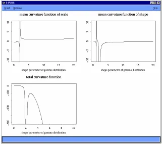
Figure 1. Location-scale, location-shape, scale-shape curvature function and mean curvature function of location.
4 3 2
3 3 3 3 3 3 3 3 3
5 4 3 2
3 3 3 3 3 3 3 3 3 3 3
4 3 2
3 3 3 3 3 3 3 3 3
where 2 10 18 14 4 ,
2 14 38 50 32 8 ,
4 18 28 18 4 4
a
b
c
3 3 3
3 2
3 3 3 3 3 3 3 3 3 3
2 2 2 2 2
3 3 3 3 3
2 2 2 2 2
3 3 3 3 3
4 ,
2 8 10 4 6 6 ,
4 4 5 2 8 8,
2 6 4 5 2 8 8,
d
e
f
2 3 2 2 2 2 3 2
3 3 3 3 3 3 3 3
2 2 2
3 3 3 3
2
3 3 3
4 4 5 6 2 12 24 16,
2 2 4 7 4 14 14,
2 5 2 2 1.
g
h
i
During the derivation of the Ricci curvature tensor, we applied the following four symmetric properties of the Riemannian Curvature Tensor:
a) ,
b) ,
c) ,
d) 0
ijkl jikl
ijkl ijlk
ijkl klij
ijkl jkil kijl
R R
R R
R R
R R R
(3.4)
Detailed proof of these four useful properties will not be given but left in references [18,19]. We will state these relations in terms of components with respect to
any basis. Relation c) states the first pair of indices and the second pair can be interchanged without altering the value of the components. Relations a) and b) state that the covariant curvature tensor is skew-symmetric with respect to the first two indices and the last two indices. The symmetry expressed in d) is called the “algebraic Bianchi identity”. Using a)-d), it is easy to show that a three-term sum obtained by cyclically permuting any three indices of R is also zero.
Let
h
1, 2, ,k
be a normal orthogonal base of tangent space TpM at a point p of the manifold M.
,
basis vectors h and h . Then, the mean curvatures
k in the direction h are defined by:
1
1 ,
1
1 1
k
i j
ij
i j
ij
k k
k
R h h
k g h h
(3.5)
In the three-parameter Gamma Distribution case, we obtain the mean curvatures for each direction of the bases.
2 2
3
2 2
3 3
2
3 3 3
1 ,
4 2
2 ,
4 2
3 .
8 1 2
where , , , , and are
defined the same as (3.3)
a e
b g
d i
a b d e g i
k
k
k
(3.6)
The scalar curvature, R, of the space is defined as the
trace of the Ricci Tensor: . As a result, the calculation discovered is the scalar curvature of our pa- rameter space:
ij ij
Rg R
3 3
3 3
6 5
3 3 3 3
4 3
3 3 3 3
2
3 3 3 3
8
3 3 3
7 6
3 3 3 3
5 4
3 3 3 3
3
3 3 3 3
.
2 1 2
where 4 32
104 176
164 80
16 4
44 208
552 900
924 584
totx toty
totx R
2
3 3 3
208 32 ,
(3.7)
3 4 3 3 3 2 3
3 3 3 3
3 2 3 2 2 2 2
3 3 3
5 4 3 2
3 3 3 3
6 5 4 3 2
3 3 3 3 3
3
2 14 36 40
16 10 8
4 28 72 80 32
4 40 164 352 416
256 64.
toty
3
[image:5.595.137.458.437.722.2]From Equations (3.6) and (3.7), notice that the mean and scalar curvatures are also a function of shape pa- rameter only. In the concluding remarks, we would like to tabulate and plot all the three sectional curvatures and mean curvatures together. In this way it would be very easy to see the common behavior of these six functions (See Figure 2).
4. List the Fundamental Tensor
4.1. This Section Shows the List for Christoffel Symbols of the First Kind of the Three-Parameter Gamma Distribution
3 2 2
3 2 3 2 3 2
2 2 2
3 2 3 2 3 2
3
3 3
2 2
2 2
3 2 2 3 2
1 1
11, 2 , 11,3 , 12,1 ,
2 2 2 2
1 1
12,3 , 13,1 , 13, 2 ,
2 1 2 2 2 1
2 3
22,1 , 22, 2 , 22,3 ,
2
1 1
23,1 , 23, 2 , 33,1 ,
2 1 2 1
3
2 2 2 2 1 1 1 (4.1)
33,3
3 . 2 4.2. This Is the List for Christoffel Symbols of the Second Kind
3 31 2 3 3
11 11 2 11 2 2
3 2 3 2 3 2
2
3 3 3
1 3 2 1
12 12 13
2 2 3 3
3 3
2 3 1
13 13 22
3 3 3 2 2
2 3
22
2 1 2 1 1
, , ,
2 2 2 2 2
2 5 4 2
1
, , ,
2 2 4 1 2
2 3 1 1 1 2
, , ,
4 1 2 2 2 2
4 1 2 3
3 33 3 1
22 2 23
2 2 3
3
3 3 3 3 3
3
2 3 1
23 23 33 2
3 2 3
3 3
3 3 3 2 3 3 3
2 3
33 2 33
3 3
2 1 2
1
, , ,
4 1
2 1
2 3 1 1
, ,
4 1 2 2 1
1 2 1 1 2
, . 1 2 1 2 2 , (4.2)
4.3. This Is the List for the Four Components Covariant Riemannian Curvature Tensor
3
3 3
1212 2 4 1213 2 3 1223
3 3
3 2 3 3 2
2 1 1
2 1 1
2 4 1
, , ,
4 1 2
2 2 4 1 2
R R R 3
2
3 23 3 3 3 3 3 3
1313 2 3 2
3 3 2
3 3
1323 2
3 3 2
2 5 8 4 7 2 4 1 2
,
8 1 2
1 1
,
4 1 2
R R
33 3 3 3
2323 2 2
3 2
3
3 3 3
2333 2
3 2
4 9 2 3 4 1
,
8 1
2 ( 1)
3
23 3
where 2 3 2 1 . While all the
other components are zero. three sectional curvature have a very flat and long tail or the horizontal axis as their common asympototic axis. This point of view could also apply to the three mean curvatures. Second, we observed that all six curvature graphs have a vertical asympototic line at either
5. Concluding Remarks
As the saying goes, a graph is worth a thousand words. After tabulating in 5.1 these seven important curvature functions as functions of the shape parameter 3, using both common values and extremes, the next step in the analysis is to plot these seven functions versus the shape parameter.
3 1 or 2
or both. For the location-scale, k(1,2), or the
scale-shape parameters, k(2,3), or sectional curvature and
mean curvature of scale parameter, k(2), there is an al-
most equilateral hyperbola. All of these three functions have a vertical asympototic line at 2 or 1. This could ex- plain Chen’s [1-3] attempts to simulate the sampling dis- tribution and power function of Cox’s [4,5] test statistics of separate families of hypotheses. He found that the Newton-Raphson iteration method could fail to converge to the required roots when real roots are close to 2 or 1. It clearly finds that the slope of the curve or surface will always switch between a very large positive and negative value. As we mention before, Johnson, Kotz and Balak- rishnan: Continuous Univariate Distributions Volume I both editions (p. 356 for second edition) has claimed that the shape parameter would be at least 2.5 or larger to avoid this nonconvergent problem. The location-shape,
k(1,3), behaves more differently for the sectional curva-
[image:7.595.56.539.394.736.2]Let us summarize the sectional and mean curvature graphs and enumerate their common phenomenona. First, we observe that there is a common result among the six functions when the shape parameter increases to positive infinity: the six functions all converge to zero, either from above or below the horizontal axes. It is a well- known fact that for shape parameters greater than or equal to 44.44, the gamma distribution nearly coincides with the normal distribution. Even if the shape parameter increase to 120, the gamma distribution would not devi- ate much from the normal distribution. Hence, we would expect to see one of two things: either the three sectional curvatures have identical values, or the graphs of the
Table 1. Shape parameter of three-parameter gamma distribution.
45 ~ 120 44.44 39.50 34.50 30.00 27.50 25.00 20.50
0.008 0.009 0.010 0.011 0.013 0.014 0.017
(1, 2) 0.268 ~ 0.256 0.268 0.270 0.273 0.277 0.280 0.283 0.291
(1,3) 0.213 ~ 0.237 0.212 0.207 0.201 0.193 0.187 0.180 0.162
(2,3) 0.254 ~ k
k k
0.260 0.260 0.261 0.263 0.265 0.266 0.268 0.272
(1) 1.838 ~ 1.782 1.840 1.852 1.868 1.887 1.901 1.917 1.959
(2) 1.234 ~ 1.244 1.234 1.232 1.229 1.226 1.224 1.221 1.215
(3) 0.271 ~ 0.258 0.271 0.274 0.278 0.282 0.285 0.2
k k k
89 0.299
766668 ~ 15166443 737767 513612 338371 219513 167499 124428 66747 R
16.00 13.50 11.00 8.50 6.50 5.50 4.00 3.50
0.022 0.027 0.033 0.044 0.060 0.073 0.109 0.129 (1, 2) 0.304 0.316 0.335 0.368 0.423 0.474 0.649 0.787 (1,3) 0.133 0.107 0.065 0.012 0.142 0.269 0.759 1.205 (2,3) 0.279 0.285 0.2
k k k
95 0.311 0.336 0.358 0.422 0.463 (1) 2.029 2.093 2.195 2.382 2.699 3.014 4.225 5.329 (2) 1.207 1.199 1.190 1.176 1.161 1.155 1.163 1.191 (3) 0.316 0.331 0.355 0.400 0.476 0.553 0.848 1.117
30388 17592 9014 3812 1
k k k R
514 838 267 170
3.00 2.50 2.10 2.01 1.99 1.10 1.01 0.99 0.01
0.159 0.207 0.269 0.287 0.292 0.829 0.980 1.020 19608
(1, 2) 1.068 1.920 8.808 86.426 86.067 0.835 0.758 0.743 0.500
(1,3) 2.279 7.009 128 11749 11509 0.352 0.258 0.24
k k
3 0.003
(2,3) 0.526 0.638 0.808 0.867 0.881 7.806 77.578 77.478 0.514
(1) 7.965 19.312 296 26234 25517 0.973 0.768 0.733 0.251
(2) 1.276 1.626 4.985 43.771 42.480 0.232 0.248 0.253 0.504
(3) 1.756 4.468 68 5914
k k k k
5715 1.648 15.352 15.040 0.001
114 123 1254 105466 101566 1.91 1.53 1.48 1
R
ture and mean curvature of location. However, while they both have asympototic lines at 2, and both converge to zero above or below the horizontal axis as the shape parameter increased to infinity. Finally, the mean curva- ture of shape parameter, k(3), has two asympototic lines
at 1 and 2, with a point of inflection near 1.44 where it switches from the positive curvature to the negative one. As the shape parameter graduately increase from 2 to in- finity, the curvature tends to zero below the axis.
The question why the “magic number 2.5” is picked. Based on Table 1 and first six graphs we draw the an- swer has appeared to be trivial. We would like to
1) For the shape parameter greater than 2.5 it is safe zone in term of slope;
2) For the shape parameter between 0 and 2.5 all the six curvature functions behaves very unstably. We found all six curvature functions except scale-shape curvature function have a dramatically changed value when the shape parameter is around to 2.01, 1.99, 1.01 or 0.99 [18- 20].
REFERENCES
[1] W.W. S. Chen, “Testing Gamma and Weibull Distribu- tion: A Comparative Study,” Estadistica, Vol. 39, 1987,
pp. 1-26.
[2] W. W. S. Chen, “Evaluation of the First 12 Derivatives of the Digamma PSI Functions with Applications,” Pro- ceeding of Statistical Computing Section, 1982, pp. 293-
298.
[3] W. W. S. Chen, “Curvature Gaussian or Riemann,” In-ternational Conference (IISA), McMaster University, Ha-
milton, 10-11 October 1998.
[4] D. R. Cox, “Tests of Separate Families of Hypotheses,”
Proceedings of 4th Berkeley Symposium, Vol. 1, 1961, pp.
105-123.
[5] D. R. Cox, “Further Results on Tests of Separate Families of Hypotheses,” Society B, Vol. 24, 1962, pp. 406-424.
[6] C. R. Rao, “Information and Accuracy Attainable in the Estimation of Statistical Parameters,” Bulletin of Calcutta Mathematical Society, Vol. 37, 1945, pp. 81-89.
[7] B. Efron, “Defining the Curvature of a Statistical Problem (with Applications to Second Order Efficiency),” Annals of Statistics, Vol. 3, No. 6, 1975, pp. 1189-1217.
doi:10.1214/aos/1176343282
[8] A. F. S. Mitchell, “Statistical Manifolds of Univariate Elliptic Distributions,” International Statistical Review, Vol. 56, No. 1, 1988, pp. 1-16. doi:10.2307/1403358
[9] J. Burbea and C. R. Rao, “Entropy Differential Metric, Distance and Divergence Measures in Probability Spaces: A Unified Approach,” Journal Multivariate Analysis, Vol.
12, No. 4, 1982, pp. 575-596.
doi:10.1016/0047-259X(82)90065-3
[10] L. T. Skovgaard, “A Riemannian Geometry of the Multi- variate Normal Model,” Scandinavian Journal of Statis- tics, Vol. 11, No. 4, 1984, pp. 211-223.
[11] Y. Sato, K. Sugawa and M. Kawaguchi, “The Geometri- cal Structure of the Parameter Space of the Two-Dimen- sional Normal Distribution,” Reports on Mathematical Physics, Vol. 16, No. 1, 1979, pp. 111-119.
doi:10.1016/0034-4877(79)90043-0
[12] R. E. Kass, “The Geometry of Asymptotic Inference,”
Statistical Science, Vol. 4, No. 3, 1989, pp. 188-234.
[13] R. E. Kass and P. W. Vos, “Geometrical Foundations of Asymptotic Inference,” John Wiley & Sons, Inc., New York, 1997.
[14] A. C. Hearn, “REDUCE User’s and Contributed Pack- ages Manual,” Version 3.7.
[15] N. Balakrishnan and W. Chen, “Handbook of Tables for Order Statistics from Gamma Distributions with Applica- tions,” Kluwer Academic Publishers, Not Publish yet. [16] N. L. Johnson and S. Kotz, “Continuous Univariate Dis-
tributions-1,” Houghton Mifflin Company, Boston, 1970. [17] N. L. Johnson, S. Kotz and N. Balakrishnan, “Continuous Univariate Distributions,” 2nd Edition, John Wiley & Sons, Inc., New York, 1994.
[18] D. J. Struik, “Lectures on Classical Differential Geome- try,” 2nd Edition, Dover Publications, Inc., New York, 1998.
[19] S. I. Goldberg, “Curvature and Homology,” Revised Edi- tion, Dover Publications, Inc., New York, 1998.
APPENDIX
The definition of the Christoffel Symbols of the first kind, in terms of the first partial derivatives of the components of the Riemannian metric tensor:
,
12
jh kh jk k j h
g g g
jk h
x x x
.
The Christoffel Symbols, of the second kind, are de- fined as the inner product of the inverse of the Rieman- nian metric tensor with the Christoffel Symbols of the first kind:
, , sum on .
i ih
jk g jk h h
The Mixed Riemann curvature tensor is defined by:
, sum on .
h h
jk
h ik h m h m
ijk im jk jm ik
i j
R m
x x
The inner product of the Mixed Riemann curvature tensor and Riemannian metric tensor,
, sum on ,
h
ijkl ijk hl
R R g h is called the Covariant Rie-
mann curvature tensor. It is a covariant tensor of the fourth order. The components are also re- spectively known as Riemannian Symbols of the first and second kind. All listed formulae can be found in the fol-lowing reference books Struik, D.J. [18] or Goldberg, S.I. [19].
and
h
ijk ijkl