An Address Based Routing Scheme for Static Applications of Wireless Sensor Networks

(1)

An Address-Based Routing Scheme for

Static Applications of Wireless Sensor

Networks

Weibo Li

A thesis submitted in partial fulfilment of the requirements for the degree of

Master of Engineering in

Electrical and Computer Engineering at the

University of Canterbury, Christchurch, New Zealand.

(2)

ABSTRACT

Wireless sensor networks (WSNs), being a relatively new technology, largely employ protocols designed for other ad hoc networks, especially mobile ad hoc networks (MANETs). However, on the basis of applications, there are many differences between WSNs and other types of ad hoc network and so WSNs would benefit from protocols which take into account their specific properties, especially in routing. Bhatti and Yue (2006) pro-posed an addressing scheme for multi-hop networks. It provides a systematic address structure for WSNs and allows network topology to avoid the fatal node failure problem which could occur with theZigBee tree structure. In this work, a new routing strategy is developed based on Bhatti and Yue’s addressing scheme. The new approach is to im-plement a hybrid flooding scheme that combines flooding with shortest-path methods to yield a more practical routing protocol for static WSN applications. The primary idea is to set a flooding counterK as an overhead parameter of control messages which are used to discover routes between any arbitrary nodes. These route request messages are flooded forK hops and then oriented by shortest-path routing from multiple nodes in the edge of the flooding area to the destination. The simulation results show that this protocol under certain wireless circumstances is more energy conscious and produces less redundancy than reactive ZigBee routing protocol. Another advantage is that the routing protocol can adapt any dynamic environment in various WSN applications to achieve a satisfactory data delivery ratio in exchange for redundancy.

Keywords - Wireless Sensor Networks; ZigBee; Ad hoc networks; Routing Protocol;

(3)

(4)

ACKNOWLEDGEMENT

Intelligent people are everywhere, but a wise man is hard to meet. I am lucky to know two wise men at one time, Professor Harsha Sirisena and Professor Krys Pawlikowski. I would like to start by thanking Professor Harsha Sirisena, my supervisor and mentor. Harsha has been a wonderful mentor in the past two years. I prefer to call him a ”Guru” who not only teaches me sciences but also influences me with wisdom. He is such a kind person who really understands and cares the students from overseas like me. I thank him for providing me many opportunities, support, encouragement and guidance. What I leant from him will be of great benefit to the rest of my life. I would also like to thank Professor Krys Pawlikowski, my joint supervisor and good friend. Krys is always energic and optimistic, which makes him a good mentor for every young man. I thank him for his energy and time invested into my research and our Networking Research Group. Krys is also my good friend. My first river rafting experience was shared with him, which was a wonderful time.

I would also like to thank my colleagues. I can always get help and new ideas from them. It was really a good time to work with them for two years.

I am indebted to my parents, Li Shigui and Shi yanhua, for everything I own now. They gave me a heart and a soul, taught me the meaning of life, the importance of family. I would like to thank them for their understanding and support, they gave me their wings and made me fly in pursuit of my dreams. They did what the best parents in the world could do.

(5)

iv ACKNOWLEDGEMENT

(6)

LIST OF FIGURES

1.1 ZigBee Network Topologies 2

1.2 ZigBee Protocol Stack Architecture 3

1.3 IEEE 802 Family 3

1.4 Vineyard Monitoring and Irrigation System 5

1.5 ZigBee Applications 6

1.6 Sensor Web 1.0 Pod 9

1.7 Hierarchical and Flat Address Spaces 14

2.1 Basic ZigBee Route Discovery Algorithm 20

2.2 Receipt of Route Request 22

2.3 Receipt of Route Reply 24

2.4 3-dimensional Hypercube Structure 26

2.5 Addressing Process in A 2-dimensional Address Grid 28

2.6 An Example of A Chain Address Structure 29

2.7 Disordered Address Assignment 31

(9)

viii LIST OF FIGURES

3.2 Implementation of Bhatti and Yue’s Addressing Scheme 37

3.3 The ABAF Network Model 38

3.4 A network section utilized for analysis 39

3.5 Shortest-path Routing 41

3.6 Partial Flooding 43

3.7 Guaranteed Message Delivery 44

3.8 The Route Discovery Process of The ABAF Routing Protocol in a

reg-ular (N+1)×(N+1) grid 47

3.9 Basic ABAF Route Discovery Algorithm 53

3.10 Receipt of Route Request in ABAF 55

4.1 Simulators for Different Application Domains 60

4.2 The Simulation Topology and The Host Internal Structure of Ad hoc Sim 63

4.3 The Connection between PHY Modules of Two Nodes 65

4.4 The Input Dialog Boxes for The Number of Columns and Rows 71

4.5 A 4×3 Static model Generated by FAS 72

4.6 The Topology with Dynamic Links Generated by The Transmitter Module 75

4.7 Delivery Ratio in A 5×5 Network with A Link Failure Probability of 0.05 83

4.8 Delivery Ratio in A 20×20 Network with A Link Failure Probability of

0.05 84

(10)

LIST OF FIGURES ix

4.10 Delivery Ratio in A 20×20 Network with A Link Failure Probability of

0.20 85

4.11 Redundancy in A 5×5 Network with A Link Failure Probability of 0.05 86

4.15 Received DATA in A 20×20 Network with A Link Failure Probability of

(11)

(12)

LIST OF TABLES

2.1 Comparison of Addressing Schemes 32

3.1 Neighbor Table Entry 57

3.2 Routing Table 57

3.3 Routing Table Entry for The Four Valid Links 57

4.1 Algorithm 1: The class setPos 71

4.2 Algorithm 2: The Modified Network Moduleworld.ned 72

4.3 Algorithm 3: The Modified PHY Module 72

4.4 Algorithm 4: The Transmitter Module 75

4.5 Algorithm 5: PHY Handles a Message from Transmitter 76

4.6 Algorithm 6: ABAF algorithm 78

4.7 Algorithm 7: The class getNexthop 79

4.8 The Old Setting of The Key Parameters 80

(13)

(14)

Chapter 1 INTRODUCTION

1.1 WIRELESS SENSOR NETWORKS AND ZIGBEE

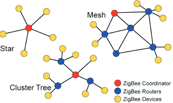
Wireless networks enable us to communicate with each other anytime and anyplace. The wireless networks commonly used are known as infrastructured networks. This type of network always employs central devices known as base stations to exchange data with mobile handsets within the transmission range. When a mobile handset moves out of coverage of a base station, a handoff process occurs to ensure the communication continues via a new base station. The other type of network is infrastructureless, called ad hoc networks. Ad hoc networks have no fixed base station: all nodes connect to each other dynamically. As defined by ZigBee Alliance, each node functions as a router to discover and maintain routes, as shown in Figure 1.1. When network components work in a mobile manner, the network is called Mobile Ad Hoc Network (MANET). MANETs focus on End-to-End communication, while the devices in static networks cooperate to accomplish some tasks. Typical examples of an ad hoc network are Bluetooth and Wireless Sensor Networks [1].

(15)

[image:15.612.109.448.61.264.2]

2 CHAPTER 1 INTRODUCTION

Figure 1.1 ZigBee Network Topologies

ZigBee is a suite of up-level communication protocols based on the IEEE 802.15.4 standard for Wireless Sensor Network, see Figure 1.2 [3]. IEEE 802.15.4 provides the base layers which includes a physical (PHY) layer and a medium access control (MAC) layer, while ZigBee defines protocols from the network (NWK) layer to a part of the application (APP) layer. The top application layer is reserved to end users.

Compared with its brother, the well-known Bluetooth which employs IEEE 802.15.1 standard, ZigBee has the properties of a long transmission range, low bandwidth, low cost, low power consumption, high flexibility and high scalability [1]. The distinctive properties of ZigBee just meet the exact requirements of particular applications and therefore make ZigBee a popular research area. Figure 1.3 illustrates the position of ZigBee in IEEE wireless space [4].

1.2 WIRELESS SENSOR NETWORK APPLICATIONS

(16)

def-1.2 WIRELESS SENSOR NETWORK APPLICATIONS 3

IEEE 802.15.4

defined

ZigBee TM_Alliance

defined End manufacturer defined Layer function Layer interface

Physical (PHY) Layer Medium Access Control (MAC) Layer

Network (NWK) Layer

-Application Support Sublayer (APS)

APS Message Broker ASL Security Management APS Security Management Reflector Management Application Object 240 Application Object 1 …

Application (APL) Layer

ZigBee Device Object (ZDO) Endpoint 240 APSDE-SAP Endpoint 1 APSDE-SAP Endpoint 0 APSDE-SAP NLDE-SAP MLDE-SAP _MLME-SAP PD-SAP PLME-SAP NWK Security Management NWK Message Broker Routing Management Network Management

2.4 GHz Radio 868/915 MHz Radio

Security Service Provider Z D O P u b li c In te rf a c e s Application Framework Z D O M a n a g e m e n t P la n e A P S M E -S A P N L M E -S A P

[image:16.612.203.538.108.333.2]

Figure 1.2 ZigBee Protocol Stack Architecture

(17)

inition of Wireless Sensor Networks, which ”consist of individual nodes that are able to interact with their environment by sensing or controlling physical parameters; these

nodes have to collaborate in order to fulfill their tasks as, usually, a single node is

in-capable of doing so; and they use wireless communication to enable this collaboration”

(pp.2). The unique characteristics of sensor nodes make WSNs highly flexible; there-fore, the range of application is very wide. Due to the immaturity of Wireless Sensor Network standards, many related protocols and technologies are currently used in WSN architecture and produces many possible WSN application scenarios. The following ex-amples are a brief overview of WSN application cases which indicate the scope of WSN applications, which are also categorized in [5] into anear-term commercial applications list according to research and application interests in the US.

• Auto Meter Reading (AMR) Wireless sensor nodes are embedded in

meter-ing devices to record and transmit data periodically. It can be often found in gas or electricity metering within a residential community range. The metering data of the whole area can be read by a handset device, without moving around. The handset device can even be mounted in a station to collect and transmit data automatically through a telephone line or the Internet.

• Environment and Agriculture Monitoring Wireless sensor nodes can be

distributed in woods, vineyards or marine farms to monitor the environmental conditions and report details. Furthermore, the sensor nodes can act as an actu-ator connected to irrigating machines to achieve automatic irrigation.

• Intelligent Buildings In complex buildings, energy is actually wasted by

(18)

1.2 WIRELESS SENSOR NETWORK APPLICATIONS 5

• Industrial Detection and Control Sensors play an important role in industry.

Wireless sensors can be dropped or fixed to areas that are unreachable or hard to access, in order to monitor industrial metrics and detect mechanical faults. Moreover some dangerous operations can be done by remote control through WSNs.

• Stock Management In supermarkets or docks, electronic labels can be attached

to shelves and containers. Warehouse managers can easily upload and download freight information by a handset or monitor and track freights by a security system based on a WSN.

Figure 1.4 Vineyard Monitoring and Irrigation System. The deployed wireless device is a node of Camalie Net which is a soil moisture monitoring system developed by UC Berkeley in collaboration with Intel Corp and commercialized by Crossbow Inc.

The potential forms of WSN are almost unlimited. Figure 1.4 gives an illustration of WSN application in a vineyard [7]. A good summary of general WSN applications can be found in Bob Heile’s tutorial [4], also see Figure 1.5.

Most of these applications share similar characteristics so that they are taxonomized into the following types in [8, 2].

• Event Monitoring and Detection Sensor nodes are required to report

(19)

Figure 1.5 ZigBee Applications

• Measurement and Actuation In this scenario, both one-to-many and

many-to-one models are involved. Nodes usually function on demand. For measurement applications, data processing is sometimes required.

• Tracking WSNs could work in MANET fashion, which means wireless sensor

nodes are mobile in particular applications. On the other hand, the sources of information can also roam around within the area monitored by a group of static wireless sensor nodes.

However, we would like to classify WSN applications according to the specific purposes of them, for we think this taxonomy matches the design goals of WSN protocols.

• Data Oriented Applications In the large scale implementations of WSNs

(20)

1.3 GENERAL DESIGN PRINCIPLES AND CHALLENGES 7

can present an intuitional result and improve the accuracy of monitoring and measurement.

• Data Source Oriented Applications For WSN applications like AMR, office

automation and stock management, each single node has its own task. Collected data need to be identified by the identity of sources. In addition, sensor nodes might act as actuators. End-to-end communication is the basis of the data traffic in this type of application.

1.3 GENERAL DESIGN PRINCIPLES AND CHALLENGES

It is evident from the last section that the design of WSNs is highly application-specific; however, the common traits of applications can lead to general challenges of WSNs design.

• Topology Control Most of current WSN applications show that sensor nodes

are stationary after they are dropped or deployed in the target area. This is an attribute that distinguishes WSNs from other ad hoc networks. The pre-configured deployment requires topology management to improve the WSNs effi-ciency according to the characteristics of applications; on the other hand, auto-configuration is crucial for the wireless sensor nodes that are randomly dropped in the field. As wireless channel interference, power availability and nodes dam-age exist all the time, topology control appears to be indispensable for WSNs to operate in the highly dynamic environment.

• Life Span In many scenarios, the energy storage of a sensor node is very limited,

(21)

to accomplish expectant missions. Rechargeable batteries can extend the life-time of sensor nodes by obtaining energy supplement from the environment (sun, vibration and wind), but it requires a backup battery and an additional power converting circuit to provide consistent power supplies [2], which will apparently lead to the increase in both the size and the cost of sensor nodes. Hence, in this scenario, the improvement of energy efficiency and lifespan of WSNs becomes the primary design goal in this scenario; in addition, power-aware protocols and mechanisms are needed, and the trade-offs against quality of service (QoS) shall be considered [5].

• Fault Tolerance Sensor nodes failure might happen due to hardware damage or

software errors. Running out of batteries and interruption of communication can also cut off sensor nodes from the whole network. Both increasing deployment density of sensor nodes and topology control can help a WSN as a whole to function correctly regardless of nodes failure.

• Cost of Wireless Sensor devices [5] To commercialize WSNs, the price of

individual sensor nodes is the key concern. The target cost of a single sensor node is generally expected to be less than $1, while the cost of a wireless sensor device based on Bluetooth technology is currently around $10. Meanwhile, the size of sensor nodes tends to be smaller: four key components of sensor devices,

a power unit, a sensing unit, aprocessor and a transceiver have to be fitted into

a 2×5×1cm3

module, as shown in Figure 1.6 [9].

• Standardization As the development of WSNs, another issue, standardization,

begins to attract people’s attention due to its direct influence on the cost and the commercialization of WSNs. In fact, the cost-effective commercial applications are being encumbered with highly application-specific protocols. A straightfor-ward design goal of WSNs is clearly given by Kazem, Daniel and Taieb (2007):

”The goal of WSN engineers is to develop a cost-effective standards-based wireless

networking solution that supports low-to-medium data rates, has low power

(22)

1.4 WIRELESS SENSOR NETWORK ROUTING PROTOCOLS 9

Figure 1.6 Sensor Web 1.0 pod, circa 1998 which includes antenna, battery, and sensors.

being implemented in the lower layers of WSNs: IEEE 802.15.4/ZigBee tend to be used in an indoor environment, while IEEE 802.11x and WiMax (IEEE 802.16) might be suitable for outdoor deployments. Since the networking layer is the characteristic that differs WSNs from traditional networks [5], WSN researchers are mainly focusing on the standardization of the routing protocols. Further-more, standardization also covers various other issues that include the protocol stack design, cross-layer design, middlewares, on-board operating systems (OS) and operation softwares in remote sinks.

The large diversity of the applications always pushes the design of WSNs to a higher level. Quality of service (QoS), energy efficiency, scalability, robustness, self-configuration and data processing capacity are all expected to be optimized; however, none of current protocol cluster is capable enough to satisfy all of these requirements.

1.4 WIRELESS SENSOR NETWORK ROUTING PROTOCOLS

(23)

wire-10 CHAPTER 1 INTRODUCTION

less networks, in which data needs to travel via a multi-hop path from a source to a destination; therefore, communication in WSNs involves more path discovery and determination. Secondly, the energy limitation of sensor nodes is the primary issue: sensing, actuator functions, data processing and communication are all accompanied by power consumption, among which the communication via wireless is the most power consumptive operation for a wireless sensor node [2, 10, 11]. Therefore a simple, robust, energy aware routing protocol should be the design goal.

1.4.1 Taxonomy of Ad Hoc Routing Protocols

Ad hoc routing protocols are mostly being developed in mobile manner, known as mobile ad hoc networks (MANETs). There are obvious differences between WSNs and MANETs. A WSN is generally composed of a group of sensor nodes, whose main task is to collect and exchange information. The communication between nodes works in three basic manners: one-to-many, many-to-one and any-to-any [8]. On the other side, the development of MANETs focuses on handling the mobility of handsets and the limited wireless transmission range. Therefore the routing protocol design should treat WSNs as a whole system to achieve certain tasks, while MANETs routing should deal with the problems of communication between any two or more mobile users [2].

As the basis of WSNs routing, ad hoc routing technologies have attracted researchers for years, and a large amount of protocols have been developed. One of taxonomy categorizes ad hoc routing protocols into Table-driven schemes and Source-initiated

schemes [12].

• Table-driven Protocols Available paths across the networks are maintained

at all times; however, such a benefit requires not only the constant broadcasting of routing information to update relative tables, but also much memory space to maintain the tables. This feature consequently leads to substantial data flooding and power consumption.

(24)

1.4 WIRELESS SENSOR NETWORK ROUTING PROTOCOLS 11

discovery process initiated by source nodes on demand. This kind of protocols are more energy efficient, because they released the resources used to broadcast and record various tables in table-driven protocols. However, a disadvantage is that a sender must wait until a path is discovered and built, which increases the latency. Furthermore, the route discovery involves messages flooding throughout the networks as well.

In addition, some hybrid routing strategies, combining table-driven protocols and on-demand protocols, are used in WSNs with cluster structures, where table-driven pro-tocols are used for local communication within a cluster, and routes across clusters are discovered by on-demand strategies [5]. The range of ad hoc routing protocols is too wide to be fully covered here. A detailed overview of existing ad hoc routing protocols can be found in the survey papers [12, 13, 14].

1.4.2 Taxonomy of WSN Routing Protocols

The general ad hoc routing protocols with mass data flooding are obviously not ideal for WSNs. Under the push by WSN applications, the categories of WSNs are not ambiguous any longer, which requires the considerations on various system architecture issues, as listed below, when designing a WSN routing protocol.

• Environment Dynamics Most of WSN applications assume that sensor nodes

are stationary after deployment, but the wireless environment itself is highly dynamic: links between nodes can be interfered easily, and sensor nodes could fail for various reasons and recover again after a while. The topologies in the

near-term commercial applications, mentioned in the last section, are mostly

predetermined; however, the structured topologies could still be fragmentized in dynamic wireless environment. Therefore, routing protocols should be robust enough to against the environment dynamics.

(25)

the WSN routing design. All routing strategies are trying to consume less energy on the basis of respective scenarios. Since transceiving is the most power con-sumptive operation in WSNs communication, improving data delivery efficiency and reducing retransmissions are the essential issues for WSN routing research.

• Data Traffic and Delivery Models The data traffic and delivery in WSNs

highly depends on applications. The traffic is convergent in most scenarios, while some are any-to-any or many-to-one (e.g. in the near-term commercial applica-tions). Data can be delivered to sinks in three ways: continuous, event-driven or query-driven [15]. Routing strategies can be optimized to suit the three data delivery models to achieve energy saving.

To address these design requirements, besides ad hoc routing, many routing schemes have been proposed specifically for WSNs, which are generally classified as data-centric, hierarchical, location-based and hybrid routing strategies offering multiple paths for flat network architecture [5, 16].

• Data-centric Routing When data is delivered through multiple paths, or

mul-tiple sensors generate same data from same monitored targets, redundancy thus to become significant; therefore, routing protocols are expected to implement data aggregation among a group of sensor nodes during data collection and delivery in a target area. The first routing protocol that reduces redundant data and power consumption by negotiation among nodes is SPIN, whose data advertisement mechanism prevents redundant data from being sent repeatedly, but does not guarantee the data delivery [17, 16]. Another milestone in the data-centric rout-ing research is Directed Diffusion, which inspired many later routrout-ing protocols despite the limitation of the only query-driven data delivery model [18, 16].

• Hierarchical Routing In the networks with flat structures, some ”gateway”

(26)

1.5 ADDRESSING SCHEMES 13

structures. They perform data aggregation and fusion by network clustering in order to decrease unnecessary transmission to the sink. LEACH [11] is one of the first and the most popular hierarchical routing protocol, whose idea of selecting and cycling the duty of cluster heads inspired many later hierarchical protocols. Its mechanism of delivering data along the cluster heads to the sink achieves a great reduction in energy consumption; however, the single-hop routing within the clusters limits the scalability of the protocol, and the duty cycling of cluster heads brings extra overhead [16].

• Location-based Routing Location-based routing protocols are primarily

de-veloped for MANETs to deal with end-to-end communication using geographical information. Since the proposal of the structured addressing scheme [19], ad-dresses could be used to identify and locate sensor nodes in a network. However, location-based routing can still be applicable in some mobile WSN applications. For instance, the sink could be a fixed Base Station (BS) with a large transmis-sion range, where sensor nodes roam in and out. The sensor nodes within the coverage of the BS can receive the location information of both themselves and their neighbors, and then they can use location-based protocols to communicate with the BS [20, 21].

1.5 ADDRESSING SCHEMES

When discussing routing technologies, the address structure and the naming system of networks can not be ignored, which are the fundamental components used to denote and find end users or messages in networking.

(27)

• Flat Addressing The majority of MANET routing protocols employ a flat

ad-dressing mechanism. In a flat network, addresses are randomly assigned to nodes; therefore, the distribution of addresses is unrelated to the network topology. Al-though the addressing process is easy, a flat address structure always makes it hard to build a path between two arbitrary nodes.

• Hierarchical Addressing A hierarchical addressing scheme can make the path

[image:27.612.109.445.437.671.2]

discovery process easier due to its systematic structure. The distribution of hi-erarchical addresses also does not need a central coordinator; however, it causes the waste of address resources if the network grows irregularly. The ZigBee tree structure is such an example that is commonly used in WSNs. In addition, net-works do not reserve addresses for the nodes roaming out of range. This feature makes hierarchical addressing more adaptable for static networks rather than for mobile networks.

Figure 1.7 illustrates the difference between hierarchical and flat address spaces [23].

(28)

1.6 DISSERTATION OVERVIEW 15

1.6 DISSERTATION OVERVIEW

As a member of ad hoc networks family, WSN technologies are largely derived from MANETs, especially routing protocols, many of them take into account specific prop-erties of WSNs. The literature review on the WSN routing protocols in this work shows that addressing and naming are usually treated as unavailable resources in the WSN routing protocols, efficient data delivery thus to become the focus of routing research instead of robust path discovery and maintenance. Bhatti and Yue (2006) proposed an addressing scheme for multi-hop networks, which provides a systematic address struc-ture for WSNs and can avoid the fatal node failure problem that could occur with the ZigBee tree structure [19]. This inspired our work in this thesis to utilize the system-atic address structure to develop a new path discovery strategy for the WSN routing protocols.

The main contributions of this work are the following:

• We have studied various routing protocols proposed in past literatures for WSNs and the respective advantages and drawbacks. We defined the problem, and then addressed the research topic of this thesis.

• We studied and analyzed the structured addressing scheme proposed by Bhatti and Yue and applied the scheme to a network model of practical WSN applica-tions.

• We proposed an adaptive flooding scheme that takes advantages of the systematic address structure, and applied our path discovery strategy in ZigBee routing protocol, thus, yielded a new routing protocol for static WSN applications.

(29)

routing protocols, the newly proposed routing protocol improves message delivery ratio by adaptively increasing redundancy in the presence of link failures.

(30)

Chapter 2 PRIOR AND RELATED WORKS

As we discussed in the previous chapter, standardization is one of the necessary con-ditions for the commercialization of Wireless Sensor Networks. ZigBee is currently the most specific and well-maintained technical standard for low-cost low-power wireless networking. A simplified version of Ad-hoc On-demand Distance Vector (AODV) al-gorithm is employed by ZigBee Specification in the path discovery, maintenance and repair process [24]; therefore, it is also used as the benchmark in this work. Moreover, the new routing protocol is built on the structured addressing scheme proposed by Bhatti and Yue. Therefore, for this chapter, we are going to study and analyze the ZigBee routing [3] and the new addressing strategy [19] in detail.

2.1 ZIGBEE ROUTING DISCOVERY AND MAINTENANCE ALGORITHMS

2.1.1 Route discovery

In ZigBee specification 2007, both multicast and broadcast are included in the routing strategies; therefore, the route discovery is performed for three situations in a ZigBee network.

• Unicast Route Discovery To find and establish a route between a particular

source node and a particular destination node.

(31)

partic-18 CHAPTER 2 PRIOR AND RELATED WORKS

ular source node and a multicast group with a common multicast group ID, for example, a cluster.

• Many-to-one Route Discovery To find and establish routes between a sink

device to all ZigBee routers and ZigBee coordinators within a given radius.

Here in the thesis, only the content of basic unicast routing in the original ZigBee specification is considered; furthermore, we also neglect the routing along the ZigBee tree structure applied while possible in ZigBee specification, because it does not adapt general network topologies.

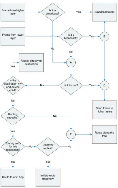
Initiation of Route Discovery

The Path Discovery process (see Figure 2.1) shall be initiated by the NWK layer of

a ZigBee router or a ZigBee coordinator, either on receipt of a ROUTE DISCOVERY request generated by the higher layer, for which there is no routing table entry corre-sponding to the destination address, or when a frame is passed in by the MAC sub-layer, for which the destination address in the routing header is not the address of the current node, the address of a valid one-hop neighbor or a broadcast address, and there is also no routing table entry corresponding to the destination of the frame. The path discov-ery is initiated by broadcasting a route request (RREQ) message to neighbor nodes. The following important fields are contained in the route request overhead:

• Source Device Address

• Destination Device Address

• Route Request ID

• Source Sequence Number

• Destination Sequence Number

(32)

2.1 ZIGBEE ROUTING DISCOVERY AND MAINTENANCE ALGORITHMS 19

In either case above, a corresponding routing table entry shall be established and set to DISCOVERY UNDERWAY. If the corresponding routing table entry exists, but the status is not ACTIVE, then the entry shall be set to DISCOVERY UNDERWAY as well.

Meanwhile, the nodes that generate route requests shall maintain a request counter as route request identifiers. The counter is incremented as a new route request is created.

A route request identifier and a source device address are used as an unique

identifi-cation (ID) of each route request frame. An intermediate node shall drop redundant request frame with the same ID. Each route request item in routing table is set with an expire timer. The expired request entries with the status of DISCOVERY UNDERWAY shall be deleted. Once a route discovery request entry is created, the route request com-mand frame is passed to the MAC sub-layer for broadcast. A route discovery request is allowed to be retried by the NWK layer for nwkcInitialRREQRetries times after the initial broadcast of the route request frame.

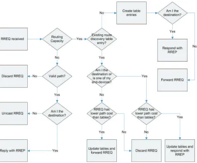
On Receipt of a Route Request

A node shall drop the route request frame if it is the destination; otherwise, it is an intermediate node and shall determine if it has routing capacity.

• Definition 2.1: Routing Capacity - A ZigBee router or ZigBee coordinator

main-tains a routing table as well as a route discovery table. Routing table entries are long-lived, while route discovery table entries last only as long as the duration of a single route discovery operation and may be reused. Routing capacity means both routing table capacity and route discovery table capacity.

In ZigBee specification 2007, the intermediate node without routing capacity proceeds the route request according to ZigBee tree routing.

(33)

[image:33.612.77.478.51.689.2]

20 CHAPTER 2 PRIOR AND RELATED WORKS

(34)

shall be created and set to expire in nwkcRouteDiscoveryTime milliseconds. Then, the node shall check the corresponding routing table entry with same destination address. If the routing table entry is not ACTIVE or does not exist, one shall be created and set to DISCOVERY UNDERWAY. The route request shall then be rebroadcasted. Other-wise, the destination sequence number in the routing table entry and the route request respectively shall be compared. If the route request has a greater destination sequence number, it shall be forwarded. If either the node is the intended destination or the destination sequence number in the current routing table entry is greater, aroute reply

(RREP) command frame shall be generated and replied along the reverse path. The route reply frame shall contain the following information:

• Source Device Address

• Destination Device Address

• Expire Timer

• Hop Counter

• Destination Sequence Number

The reverse path is automatically set up by the route request. As the route request message travels from a source to a destination, each node on the path records the address of its upstream neighbor node, from which the first copy of the route request was received. Each reverse path entry maintains an expire timer, which shall be set at least long enough for a corresponding reply message is generated and reaches the source device.

(35)

[image:35.612.83.474.210.533.2]

(36)

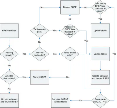
On Receipt of a Route Reply

In ZigBee specification 2007, the intermediate node without routing capacity proceeds the route reply according to ZigBee tree routing.

If the intermediate node has routing capacity, it shall check whether it is the destina-tion of the route reply frame. If positive, it shall search its route discovery table for the entry corresponding to the route request ID in the route reply frame header. The route reply frame shall be dropped, if a route discovery table entry does not exist. Oth-erwise, the node shall search its routing table for an entry with a destination address same as the responder address in the route reply command frame. If no such routing table entry exists, the route reply shall be discarded, as well as the corresponding route discovery table entry. If the routing table entry exists and has the status of DISCOV-ERY UNDERWAY, it shall be set to VALIDATION UNDERWAY. The last hop of the route reply frame shall be set in the next hop field in the routing table entry. The path cost recorded in the route reply frame shall be inserted in the routing table entry. If the status of the routing table entry has been ACTIVE or VALIDATION UNDERWAY, the node shall compare the path cost in the route reply command frame and the routing table entry, then, either update the routing table entry by the smaller one in the route reply frame or discard the route reply with a larger path cost.

If the device is not the destination of the route reply, it shall repeat comparison process above and update corresponding information field. If the route entry is updated, the node shall search the route discovery table for the next hop address corresponding to the route reply, compute the link cost, update the route reply frame and forward the route reply to the destination. Figure 2.3 illustrates how to process a route reply

2.1.2 Route Maintenance

(37)

[image:37.612.78.477.188.556.2]

(38)

2.2 A STRUCTURED ADDRESSING SCHEME 25

a time-windowed scheme shall be employed. Repair operations are highly unrecom-mended, because they may flood the network and cause traffic disruptions.

If a link failure happens while the node is transmitting a message via an unicast route, the node upstream of the broken link shall send a message with a network status frame back to the source to indicate the reason for the failure, and a NLME NWK STATUS indication shall be passed to the next higher layer to indicate the link failure at the same time. On receipt of a network status command frame indicating a link failure, the node shall remove the routing table entry corresponding to the original destination of the forwarded messages, and also inform the next higher layer of the failure using the same NLME NWK STATUS indication. Upon receipt of a link failure notification, the original node shall restart a path discovery process if the path is still required.

2.2 A STRUCTURED ADDRESSING SCHEME

(39)

between devices, so it happens that one parent node exhausts its address pool while other parents have addresses unused. A new device will not be able to join the network if no parent node with spare addresses is within its transmission range [3]; in addition, the waste of address space still exists in the irregularly growing networks [19].

2.2.1 Scheme Description

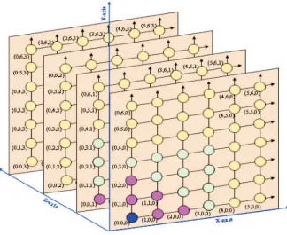
[image:39.612.115.439.290.555.2]

Bhatti and Yue have recently proposed a new addressing scheme [19]. This scheme treats the entire address space as a n-dimensional hyper-cube. Figure 2.4 shows a 3-dimensional address cube.

Figure 2.4 3-dimensional Hypercube Structure

The following annotations should be aware:

• Hyper-Cube The regular shaped cube, for example the 3-dimensional cube

(40)

• n_-dimensional _{In the} _n_{-dimensional structure, each intersection represents a}

node that has a Cartesian coordinate as its address. n is also the number of address components that is a pre-configured parameter. For example, if n is 3, the address will be (x, y, z); hence, a node in then-dimensional cube can have a max ofn child nodes, which are (x+1, y, z), (x, y+1, z) and (x, y, z+1) for the given example, also see Figure 2.4.

• Address Structure The new address assigning scheme provides hierarchical

systematic address patterns.

The newly proposed addressing scheme states such advantages and advancements:

1) Addresses are allocated in a systematic manner. The address space is regular and hierarchical.

2) The waste of address resource is reduced. Even if the physical location of nodes was not uniformly distributed, the mechanism would still try to assign addresses in a regularn-dimensional pattern.

3) No flooding of notification of assigned addresses throughout the networks, and no flooding of address tables.

4) The robustness against network partitioning due to parent nodes failure is en-hanced.

5) The restriction on the depth of address hierarchy in ZigBee Tree structure is removed.

(41)

in the first case is 28_{; hence, the address range is from (}_{00, 00}_{) to (}_{FF, FF}_{). A network}

[image:41.612.134.416.129.369.2]

starts at the origin point of the Cartesian coordinates, (0, 0), and grows along any axis corresponding to the physical distribution of the nodes.

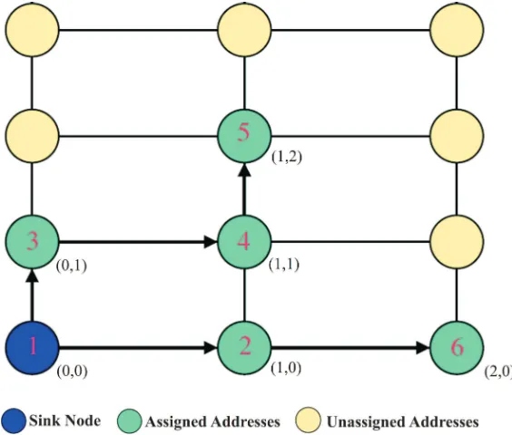
Figure 2.5 Addressing Process in A 2-dimensional Address Grid. The numbers in nodes denote the order that nodes join in the network, while the arrows represent the successive relationship of addresses.

The addressing process is illustrated in Figure 2.5 and works by following the steps below:

Step 1) We assume both of the address components are 8 bits long. The origin node, sayN0, could be not only (00, 00) but also any of the other three corners of the

grid, (00, FF), (FF, 00) and (FF, FF). (00, 00) is used here for convenience.

Step 2) A parent node only has the addresses, which are adjacent to its own address, available. The corresponding address components of the new address are either greater or equal to the parent address. For example, the first node N0

has a new child nodeN1 joined the network. The addresses available to assign

to N1 are (00, 01) and (01, 00).

(42)

y) by node A (x-1, y), the new node is now responsible for sending a message to the other potential parent node B (x, y-1) to claim that the address (x, y) has been occupied. In general, a new node in an-dimensional address space theoretically hasn potential parent nodes, but only one is going to build the actual relationship with it, and then the other n-1 potential parent nodes need to be notified. In Figure 2.5, when node 4 joins in the network, both node 2 and node 3 could be its parent node. If node 4 is assigned an address (1, 1) by node 3, it must send a message to node 2 to claim the occupation of the address (1, 1).

The address pattern would grow irregularly into a chain or a random shape, if addresses were assigned along a single axis. Figure 2.6 gives an illustration.

1 2

3 4

(0, 0)

(1, 0) (2, 0) (3, 0)

(0, 0)

(1, 0) (2, 0) (3, 0)

1 2 3 4

1 2

3 4

(1, 0) (1, 1) (0, 1)

(0, 0)

(1) Physical topology of a network (2) The chain shape address pattern of the network (3) The expected address pattern

Figure 2.6 An Example of A Chain Address Structure. The number denotes the order that nodes join in the network. The dash lines indicate possible links between nodes. As we can see, although the physical locations of nodes are in a grid pattern, the address structure grows in a chain by assigning addresses improperly.

A simple strategy is suggested by the authors to ensure a more uniform address dis-tribution. If both address components are either even or odd, the next address to be assigned should be along one available axis; otherwise, the address should be assigned along the other axis. For example, node(2, 2)and node(3, 5)will try to assign(3, 2)

and (4, 5) to their child nodes respectively, and node (1, 2) and node (2, 3) will try

(43)

2.2.2 Discussion

Despite all the advantages, problems and defects still exist in the new addressing scheme. Some issues arose while we applied it. Because these issues do not cause much impact on this work, we are not going to discuss them in detail in this thesis. They are listed below.

• The scheme claims to be able to adapt any forms of ad hoc networks; however, the practical implementation shows that it is not flexible and even not feasible in highly dynamic environment like MANET, where nodes join in and roam out randomly, see Figure 2.7. It would work well if addresses were allocated after the deployment of nodes.

• The scheme does not advice whether addresses will be reserved for nodes parti-tioned from parents, and how to reserve the addresses if the answer is positive.

• The method to prevent networks from growing irregularly was proposed by the authors; however, applying it in a n-dimensional structure could be a problem when the number of address components,n, is bigger than 2.

• Both the pre-configured n and the start points on the corners of an address structure have a negative impact on the flexibility of the addressing scheme.

(44)

1 2

3

4

5

6

7

(0, 0) (0, 1)

(1, 0)

(Null)/(3, 0)

(1, 1)

(2, 0)

(Null)

Actual Link between Parent Node and Child Node

Unsuccessful Link due to The Lack of Address

The Order That Nodes Join in the Network

[image:44.612.178.465.217.482.2]

3

(45)

[image:45.612.83.471.139.416.2]

deployment is done before the addressing; hence, the addressing scheme primarily suits our scenario for static WSNs applications.

Table 2.1 Comparison of Addressing Schemes

Flat Addressing

Schemes

Hierarchical (Binary Split)

Hierarchical (ZigBee Tree)

The New Scheme

Addressing

Process Easy Medium Medium Medium

Flooding

Overhead High High High Low

Address

Structure Irregular

Irregular if addresses borrow among

nodes

Systematic Systematic

Waste of

Addresses Low

Reduced by addresses

borrow

High in irregularly

growing networks

Low

Robustness against Network

Fragmen-tation

(46)

Chapter 3 ADDRESS-BASED ADAPTIVE FLOODING (ABAF)

ROUTING PROTOCOL

3.1 MOTIVATION AND PROBLEM DEFINITION

The state of art in WSN routing protocol research was briefly introduced in the first chapter. The traditional routing algorithms for ad hoc networks are usually categorized into PROACTIVE and REACTIVE; meanwhile, protocols specialized for WSNs are proposed in terms of data centric, direct diffusion, hierarchical, geographical routing. Although some of them are Internet Engineering Task Force (IETF) protocols, to the best of our knowledge, none of them are employed by the near-term commercial WSN applications as an industrial standard. The routing algorithm specified in the ZigBee specification is a simplified AODV combined with a table-driven strategy and tree-structural routing [3].

(47)

34 CHAPTER 3 ADDRESS-BASED ADAPTIVE FLOODING (ABAF) ROUTING PROTOCOL

failures and channel interferences, routing is no mere a ”checker game” with a clearly visible ”chessboard”, but a more complicated ”labyrinth game”. To survive in this tough environment, the scenarios of most WSN routing schemes require much extra information that is exchanged by flooding throughout the network. The information like node locations, device status (e.g. power level) are all acquired at the cost of overhead or other energy consumptive options (e.g. GPS in geographical routing). Some massive flooding could cause traffic congestions, for example, the synchronization of routing tables and address tables.

Known links to the parent node and neighbors

Unknown links across the network to the destination

Source Device

Destination Device Parent Node

Neighbor Node

Figure 3.1 A new joining node knows nothing about the network except its parent node and neigh-bors. The routing protocol design should be from the point of view of a node not an observer.

(48)

3.2 SCHEME SCENARIO 35

cost of maintenance can be low in a comparatively constant wireless channel, but the robustness decreases in an dynamic environment where link failure and node failure exist. Flooding and single-path routing are two extreme cases of routing methods. Although they are simple, their performances in terms of energy efficiency, delay and success ratio are likely to be poor.

On all accounts, nodes have to consider how to find a balance between performance and energy-efficiency [2]; therefore, new routing strategies are required to be capable of effectively managing the trade-off between optimality and efficiency [5]. Based on this standpoint, a preparatory strategy is proposed, which generates a partial flooding targeting the direction of the destination, and then takes advantage of shortest-path algorithms to reduce the redundancy in path discovery phase. The partial flooding and the shortest-path algorithms are developed based on the systematic address pattern. A parameter is set to control the partial flooding by changing the number of hops of flooded packets so that the whole route discovery process can be adjustable and flexible to adapt various wireless environments and achieve a satisfied balance between performance and energy efficiency.

3.2 SCHEME SCENARIO

3.2.1 Network Model

Fornear-term WSN applications, the sensor nodes are stationary after deployment, for

example, a vineyard irrigation and monitoring system, a stock or dock management system. when containers can be moved and the irrigation devices in the field might be damaged, the network environment can be dynamic. The network model of our Address-Based Adaptive Flooding ABAF routing protocol is such a static network operating in a dynamic wireless environment.

• Definition 3.1: Static Network - A static network is a network that all its

(49)

with each other.

• Definition 3.2: Dynamic Network - A Dynamic network is a network with link

failure and node failure that can cause local topological changes.

A single node failure makes all its incoming and outgoing links disconnected; therefore, for the convenience of analysis, only link failure is considered in the scenario.

In the near-term WSN applications, data delivery modes are usually event-driven or query-driven , and data traffic is mainly one-to-one and many-to-one (one-to-many). To improve the end-to-end route discovery efficiency, data traffic runs in the one-to-one mode in the scenario.

• Definition 3.3: Event-driven - Data transmission is triggered by local events,

for example, the temperature or humidity level in soil.

• Definition 3.4: Query-driven - Data transmission is triggered by a query from

sink(s). For instance, A sink can send a command to execute irrigation or a request for a report of freight information of the corresponding containers.

• Definition 3.5: One-to-one- Communications between any two arbitrary nodes.

The process of message delivery could involve the aid of intermediate nodes.

• Definition 3.6: Many-to-one - The many-to-one mode is assumed to be

com-posed of many one-to-one communications. Data aggregation is not considered in many-to-one mode in the route discovery phase.

Bhatti and Yue’s structural addressing scheme is employed in the ABAF routing pro-tocol as the basis of the network model. The address model follows the assumption below:

• Assumption 1: The address pattern of the network model is a 2-dimensional

(50)

grid has an unique Cartesian coordinates. The address space starts from the origin (0, 0) that can be any of four corners of the Cartesian coordinates grid. The size of the address space is(N+1)×(N+1).

In WSNs, sensor nodes are usually deployed in a certain density to ensure system reliability. The redundant deployment also makes it possible that nodes can always be divided into a group of four neighbor nodes to form a quadrangular grid in any cases, see an example shown in Figure 3.2. It can be deduced that Bhatti and Yue’s structural addressing scheme can fit in any random 2-dimensional topology. What needs to be emphasized here is that the address pattern is a logical image, while the topology of the network model is a physical structure. Based on the conclusion above, to generalize the network graphs of various applications, the following practical assumption on the physical topology of the network model is made.

• Assumption 2: The physical topology of the network model follows exactly the

same shape as the logical pattern of the address space.

(0, 0) (0, 1)

(1, 0) (2, 0) (2, 1)

(1, 1) (1, 2)

(0, 2)

a) A random sensor nodes deployment _{b) The address assignment by Bhatti and Yue's scheme}

Figure 3.2 Implementing Bhatti and Yue’s Addressing Scheme in an arbitrary topology

(51)

[image:51.612.137.420.60.350.2]

Figure 3.3 The ABAF Network Model. The topology of ABAF network model, as well as the address structure.

As noted above, the work focuses on investigating the communication between any two arbitrary nodes, assumed to be the origin(0, 0)and the end point(N, N). The network model can actually be an arbitrary section extracted from a larger network, as shown in Figure 3.4.

3.2.2 Network Configuration

The deployment and addresses assignment of sensor nodes are pre-configured following the network model shown in Figure 3.3. Miscellaneous Network Configuration

Assumptions are summarized as below:

Assumption 3:

(52)

A Larger Network

The section that we use for analysis

Figure 3.4 We can utilize an arbitrary section in a network for our analysis.

probability is considered, which is given byp.

2) The network model is composed of (N+1)×(N+1) sensor nodes as shown in Figure 3.3. No more nodes roam in or out during the simulation.

3) The density of sensor nodes deployment is high enough so that the transmission range of each node can cover all of its one-hop neighbors.

4) The distance between neighbor nodes are same due to the pre-configured topology; thus, every hop takes same time.

5) Direct communications can only occur between nodes that are directly linked, which is for the convenience of simulation.

6) All events happen in a time order in the simulation; Therefore, the wireless en-vironment shall be kept still once a message exchange begins, which means the transmission power shall not be changed and no more nodes or links fail during a message travels to the next hop.

7) An end-to-end routing discovery process from (0, 0) to (N, N) is investigated in this work.

(53)

9) The energy dissipation of transmitting and receiving are approximately assumed to be equal, although the latter is higher in many practical WSNs [2].

3.3 SCHEME DESCRIPTION

AODV has a redundant route discovery process of flooding RREQ, which ”overkills” static WSNs, while shortest-path routing is obviously less robust in a dynamic envi-ronment. The description of the ABAF routing protocol starts from implementing shortest-path routing and flooding in the defined network model. Thereafter, the im-pacts on shortest-path routing by flooding in the presence of link failure is investigated. A hybrid adaptive approach for static WSN applications is eventually proposed.

We state the following four main merits of the new proposed theABAF routing scheme.

1) Fit WSNs with a systematic address space. Addresses become practically available resources for the WSN routing.

2) The path discovery process is adaptive. A controllable parameter is employed to keep the balance between energy efficiency and QoS. Less redundancy is generated while achieving the same latency as AODV.

3) Lower redundancy. For no extra information like nodes locations or the duty of cluster heads is needed, much less broadcast of exchanged information is involved; in addition, the size of overheads is also kept small.

4) Lower cost of route maintenance. Due to the merit of the systematic address struc-ture, the size of routing tables and address tables can be reduced dramatically.

3.3.1 Shortest Path Phase

(54)

3.3 SCHEME DESCRIPTION 41

Step SP1) A message from a source node (0, 0) arrives at an intermediate node(x,

y), for example. The destination of the message is (x+n, y+n).

Step SP2) The intermediate node shall compare each corresponding address

compo-nent of the destination with its own address. Here, the compared pairs shall be respectively x and x+n,y and y+n.

Step SP3) The result of the comparison shall lead to a decision on the next hop to

the destination(x+n, y+n). In this case, three choices are available,(x+1,

y),(x, y+1) and a random choice among these two.

The repeat of the path decision process will finally lead to three simple routing methods, all of which produce a shortest path, see Figure 3.5.

• X-Y Routing A message from the source node(0, 0)is forwarded alongX-axis

orY-axis until it arrives at the edge(x+n, y)or(x, y+n); thereafter, it will reach the destination node (x+n, y+n) along the other axis.

• Zigzag Routing Messages travel in a zigzag pattern. When they can not go in

zigzag fashion any longer, they go along the appropriate axis to the destination.

• Random Walk Messages choose their next hop along X or Y direction

ran-domly. If they reach an edge ahead of time, they are routed to the destination along the appropriate axis as above.

(0, 0)

( ,N N)

(0, 0)

( ,N N)

(0, 0)

( ,N N)

X-Y Routing Zigzag Routing Random Walk

(55)

3.3.2 Partial Flooding

As we stated, the shortest-path routing algorithms are based on the scenario in the absence of link failure. It obviously consumes the least resource to deliver data between two nodes; on the other side, it has the lowest robustness against network dynamics. In the systematic address structure, the three shortest-path routing methods orient messages according to the addresses, so does flooding.

Step PF1) A message to the destination(N, N) is generated by the APP layer of the

source node (0, 0) and passed to the NWK layer for broadcasting.

Step PF2) Upon receipt of the message, the NWK layer shall compare each

corre-sponding address component of the destination with the source address

(0, 0). Here, both of the compared pairs shall be0 andN.

Step PF3) The result of the comparison shall lead to a decision on the direction

of flooding. As each node has maximum four links along x and y axis. Broadcasting from a node (x, y) thus to be divided into four multicast sections, (x+, y+), (x+, y-), (x-, y+) and (x-, y-). In this case, the message shall be set as a multicast packet with the multicast address(x+, y+), and flooded to the next hop neighbors, both (0, 1) and (1, 0).

The multicast messages shall be flooded within the configured section and finally reach the array where the destination node (N, N) is. The partial flooding is illustrated in Figure 3.6.

The partial flooding fills the triangle area in between (0, 0),(0, 2N) and (2N, 0). All nodes on the border of(0, 2N) to(2N, 0), where the destination node(N, N)is, satisfy the equation below.

(56)

(0, 0)

( ,N N)

(0, 2 )N

(2N,0)

Flooded area

bypartial flooding

[image:56.612.201.432.55.277.2]

Flooded area by full flooding

Figure 3.6 Partial Flooding. Partial flooding based on the systematic address structure

The large square is the area that a normal flooding would fill in; the small one is the (N + 1)×(N + 1) section employed for analysis in our work.

Figure 3.6 shows the message arrives at the node (N,N) in the absence of link failure. If the two links, which are in the incoming direction of the message, failed, a further flooding would still be able to ensure the message delivery from the other two links of the destination node (N,N).

Proposition 3.1: In the absence of link failure, the distance of partial flooding from a

source node (xs,ys) to a destination (xd,yd) is (xd−xs) + (yd−ys)

hops. According to the network configuration assumption 4, flooded messages shall arrive at the nodes that have equidistance to the source, the flooded area thus to be the triangle in between (xs,ys),

(0, (xd−xs)+(yd−ys)) and ((xd−xs)+(yd−ys), 0). In the presence

of link failure, (xd−xs) + (yd−ys) + 2 hops flooding can guarantee

the message delivery.

Proof: In the absence of link failure, messages can reach the destination node via

(57)

incoming links are broken at worst. Then (xd−xs) + (yd−ys) + 1 hops can

reach all four neighbors of the destination node, and one more hop can deliver messages to the destination via any of the other two links if the node is still accessible. Figure 3.7 gives an illustration.

(0, 0)

( , )1 1 ( , )2 1

( , )1 2

( , )0 1

( , )1 0

S

D

[image:57.612.194.355.177.363.2]

S Source Node D Destination Node

Figure 3.7 Guaranteed Message Delivery. To avoid confusion, the arrows only denote the route of the messages to the destination instead of the whole flooding routes. Since the links from (0, 1) and (1, 0) are unavailable, messages are flooded to (1, 1) via (1, 2) or (2, 1).

As we can see in Figure 3.6, because messages are forwarded by multicast instead of broadcast, even if we would not implement any other algorithms to make futher im-provement, the redundancy produced by the partial flooding has already been reduced to a quarter of the full flooding in AODV path discovery process.

As in ZigBee routing, redundant identical messages shall be dropped. If a message with the same ID and source address has been received before, the link cost field shall be compared. The one with lower link cost shall stay in the route discovery table, the other one shall be discarded.

(58)

3.3.3 Hybrid Adaptive Flooding

In our scenario, the partial flooding floods only a quarter area as a full flooding, which means redundancy and energy consumption are also reduced to a quarter; however, in a WSN with a steady wireless channel, the partial flooding still appears excessive; in addition, in the case that a source and a destination are respectively located on the opposite corners of a network, the partial flooding does not differ from a full flooding. In this section, we are going to discuss a hybrid approach which implements the par-tial flooding with the cooperation of the shortest-path routing to reduce routing cost further. Whereafter an adjustable parameter of flooding hops is used to control the partial flooding and make it adaptive.

For the shortest-path routing, a single hop failure means that the whole path fails. In a WSN with a single-hop failure probability p, the probability of path failureP over n

hops can be easily obtained as below.

P = 1−(1−p)n (3.2)

It is clear that, to reduce theP, either messages are delivered over less hops, or mul-tiple individual routes are provided accessible to the destination. The probability of a successful delivery via muncoupling paths thus to be

Ps= 1−Pm = 1−[1−(1−p)n]m (3.3)

(59)

To have a control on the flooding, we define a key parameter in the route request frame:

• Definition 3.7: Flooding Counter K - K is configured at a source node as an

overhead parameter of a route request command frame to control the range of flooding. K decreases by 1 after each hop, and counts down to 0 after K-hop, and then flooding is consequently over.

• Definition 3.8: Tier K - At the end of theK-hop partial flooding, route request

messages reach an array ofK+1 nodes, which is calledTier K, as shown in Figure 3.8. All K+1 nodes on theTier K have the following common property.

|XK−xs|+|YK−ys|=K (3.4)

Where (xs, ys) is the source address, and (XK, YK) is the address of a node on

theTier K.

For the flooding counter K is applied to the partial flooding, the proposed

Address-Based Adaptive Flooding (ABAF) routing protocol is accomplished. In the ABAF

routing protocol, route requests are flooded forK hops to the tierK, and then routed by the shortest-path routing fromK+1 nodes at the edge of the flooding area to the des-tination, see Figure 3.8. The redundancy involved in the path discovery is controllable so as to adapt the wireless environment. As mentioned in the previous section, fol-lowing the partial flooding, three optional shortest-path strategies are available. They show different properties while a common destination is accessed via multiple paths in the systematic topology.

• X-Y routing The load obviously gathers on the edge of the topology.

• Random Walk Two paths originating from two adjoining nodes on the tier K

(60)

• Zigzag Compared with the other two routings, it provides the minimum number

of overlapped hops, which ensures the diversity of the multi-paths.

L

3

L

1

[image:60.612.148.490.115.461.2]

L

2

Figure 3.8 The Route Discovery Process of TheABAFRouting Protocol in a regular (N+1)×(N+1)

grid

For what is supposed to be investigated is how the partial flooding and the shortest-path routing interact, it actually does not matter which shortest-path method is employed after the partial flooding. Among the three shortest-path strategies, Zigzag strategy creates routes with the least overlaps and the highest robustness, but it is the most difficult to be generalized to a mathematical model; whereas, X-Y routing produces simpler and more regular paths for analysis, as shown in Figure 3.8; hence, X-Y rout-ing is used for the analysis of the successful message delivery ratio. The followrout-ing proposition is made.

(61)

disconnected. Since X-Y routing gathers the load on the edge of the section, one link failure on the edge will break all the routes over it, while having no impact on the routes behind it. This concludes that each different link failure circumstance on the edge shall be considered and summed up to calculate the successful delivery ratio, i.e., in Figure 3.8, the failures of paths overL1,L2 andL3 shall all

be counted.

In addition, due to the inherent redundancies in flooding, a reasonable assumption is made here.

• Assumption 4: In the partial flooding stage of the path discovery process, link

failures are not considered.

Consequently, to deduce the successful delivery ratio of a route request message, only the multiple shortest paths between the tierK and the destination (N,N) need to be considered.

An example is given here, both to prove the proposition 3.2 and to explain the following derivation.

Example: In an given 8×8ABAF network model with the link failure probabilityp,

the source node (0, 0) needs to communicate with the destination node (7, 7). While the route request message is transmitted for different distance by the partial flooding, what is the corresponding successful delivery ratio

Ps?

Derivation:

The different distance that the route request is flooded for means the different value of the flooding counter K; therefore, the corresponding successful delivery ratio can be expressed as the following formulas of the link failure probability p.

(62)

successfully only if each single hop was successful.

Ps= (1−p)14 (3.5)

When K=1, the path is actually a Y pattern. The whole path would failed if the overlapping links failed or both of the non-overlapping parts failed; consequently, the formula shall be

Ps= 1− {[1−(1−p)6] + (1−p)6[1−(1−p)7][1−(1−p)7]} (3.6)

When K=2, referring Figure 3.8, route request messages are unicasted from three intermediate nodes. On the edge, both the failure of the path over L2 and the failure

of the path over L3 shall be calculated.

Ps = 1− {[1−(1−p)5] + (1−p)5p[1−(1−p)7]

+(1−p)6[1−(1−p)7][1−(1−p)6][1−(1−p)6]} (3.7)