Two topics in the theory of optimal trajectory analysis

TWO TOPICD I:N '1'HE THJi:ORY Olil OPTIMAL TH,A,JE:C'J.lOHY J\NJ\INSIS

by

G.H .. IJ\WDEN

Two 11_{opi.cs in the ~:}1_{heory of Optimal Trajectory .Analysis} By

G .. H.. I.~awden

P.ART I ~ Review of Basic Theory. 1 .. Introduction ..

2, The Mayer Problem.

PART II - Trajectory Optimization f'or a Rocket with a Generalized Thrust Characteristic.

1 .. Introduction .. 2. General ~rheo:ry.

3 .. 'rh.e Constant Pield.

J.~ .. ~rhe One Dimensional Case ..

5 .. Sounding Rocket ..

6., The Constant Power Case ..

7. Further Consid.erations ..

PAR'l' III ... Optimal 'l'raj ector•ies f'or ·a Solar Sail Vehicle .. 1 .. Introduction.,

2 .. It'orce on a Reflecting Surf'ace.,

3 .. It'light in a Unif'orm Field ..

!.~., Inverse ~1quare Ii'ield . ., The gquations of Motion ..

5.. Boundary Condit ions"

6., MinimtUn Time ].flight ..

7• 'rhe Weierstrass Condition.

B.. Zero Order Solutitin.

9. An Approximate Solution Satisfyi!l{:S the Bound.ary Conditions .. 10" General Conic Solution.

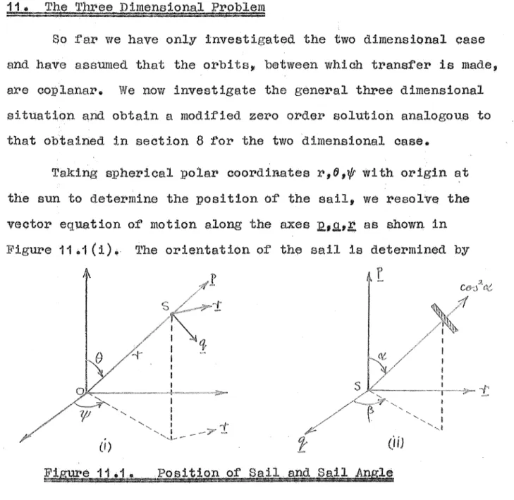
11 .. The Three Dimensional Pr•oblem. 12., Some Numerical Results ..

P.ART I

1 • Introd.uct ion

The work pl:lesented in this thesis is conoevned with

certain problems in the domain of optimal trajectory analysis. The general problem in this field is to determine the 'best' way to use a certain travel vehicle to carry out some

particular mission. Thus our vehicle may be a rocket which is designed to operate with constant exhaust velocity or at

constant powei'. Our mission may be to ef'teot a transfer f'rom the orbit of' the Earth to the orbit of some destination planet within the solar system. And our criterion, for judging which manner of' utilizing our travel vehicle is 'best' may be the requirement that the fuel consumption oJ:l the tr•ansit .time be ·minimized,

The work which follows consists basically of' thvee parts. In Part I the well kn.Own problem in the Calculus. of Variations known as the Mayer Problem is outlined, since this is the basic mathematical tool which will be used in Parts II and III. In Part II an investigation ia made of' the thrust programmes

obtained when the t:b.rust characteristic o£ a rocket is of' a more general nature than the constant exhaust velocity thrust charac•

te~istic which, for instance, is assumed throUghout in [1]. It ie shown how well known results for the case of' a rocket

operating at constant exhaust velocity may be obtained as limits of the more general results obtained in that part. Also, the

the one dimensional case. In Part III- the travel vehicle considered· is the so-called • solar' sail • • The thrust tor this vehicle is derived from the radiation pressure of the solar radiation reflected from the sail sur:f'ace. For a vehicle of this type, the question of minimizing f'uel consumption does not aro once the vehicle has been assembled in epace1 so that the

payoff criterion of most interest will be minimization of transit time. A more detailed conspectus of' the problems considered and the results obtained is presented in the separate introduotions to Parts !I and III.

A basic tool used in tackling problems of trajectory

optimization is the solution to the Mayer Problem in the

Calculus of' Variations. Following section 1.3 of [1], we out-line first a forornuletion of the Ma;ye:f:l problem wh:tch is

also anothel:' formulation of the Mayev :pvoblem which will be au.ff'iciently general to meet the requirements of' section 1 0 of

Part III.

The .first :eo:~Jmulation of' the May~~ pl~oblem :pro<~~'iH!Ids as follows. We are given n first order dH'ferential equations

(1 )

to be satisfied by thf.} n function .tt

1(t) (i=1,e, ... ,n), known as the §,..t!!ll,te Vftltia,bJ.,9i1 e.nd m :C'Wlotions aj ( t) ( j

=

1 12, .. •., ,m), known

i~atives with respect to an independent va.riable t. i.£lhese equations are ·to be valid.

f'o:r- t0

<

t

<

t1 and the

'\J

are de:f'ined throughout thiiJ iut.Gx·val as continuous functions apart f':c-om a f'inite number of finite continuities., The initial values of the xi at t

=

t ₀ are

specified by the equations

x:i

_..

=

;xio • The :J;'unctions O''j (t) and x

1 ( t) are req'ttil"ed to satisf'y certain constraining equations

(2)

(3)

where k

=

1 ,2~ •~> • •P < m and the gk a:re continuous and :possess continuous pa.r·tial cler:Lvati vee of su:ff'iciently high ovder in all their arguments. The of certain

and g

<

n. The control functions are arbitrary within the

limits impo~ed by equations

(3),(4).

The existence of control f'unotiona satis.fying the constraints

(3),(4)

will be assumed.

Let '~q+

1

_{, 1} ,:x;q+:a

,i ; "•.

,xn₁ be the values

crt:

the ~i

at

t

=

t₁ not fiXed by the constraints (4). TJJ.en our problem is to find (lGrtt:r,>ol .functions «j determining the xi so that the constraints (3), (4) are satisfied and also so that a given functional

is minimized, where t ₁ ma;v o:P may not be pre specified. J is supposed to be continuous in all its variables and to possess continuous pal'tial derivatives of' auf.ficiently high order.

We

introduce cel'tain auxiliary functions A

₁

(t), ~k(t) known as Last&nge mult}J2lier.s and a quantity F known as the Lagrapg~

eXJ.?;reasipp. defined by the equation

where we have adopted the 1J.SUal smnmation conventions indices

repeated in a produot imply summation o~er the range of the

ind~x. We are now able to state first necessary, conditions fo:tl

a minimum of J.

At poin;ts whe~e the aj are continuous, the Le.g:t•ange

multipliers ~ ,JJ.k must satisfy the dif'terential· equations

and the equationa

For the so-called no:rmaf.. ,l2~oble~ we e,lso have boun.dal'y

conditions of the fo~m

a

=

q+1,. •. ,n

Equntiona (1 ), (3)1 (7), {8) :provide a set of 2n+ m+ p

(8)

(9) (1 0)

equa:t:i.ons be isf':i.ed by the same number of :runotions xi (t),

aj(t),A1 (t),JJ.k(t)., Eq_uations (2), (4), (9), (10) provide 2n+1 end co:ruli tiona which ser·v~ to determine the n constants "io, the n

constants of integration associated with the differential

equations ( 1 ) and the end point \ •

At a. col;lnen:- on an opt~.mal trajectory~ where some or all of' the a~ discontinuous, we may apply the Weierstrass•

Elrd:mann Corner Conditions •. These state that at a corner, the

Lagrange multipliers ?\i and the expression "i*i must all be

continuous.

A first integral of equations (1

),(7)

exists when the

functions :ri,gk are not explicitly dependent upon t. !t is given by the equation

1\i:X:i

=

constant. (11)

that :ror• a minimmn of' J, the inequality

must be satisfied a.t every point on the minimal t!'ajeotory, J:n this inequality, the quantities "-:t,xi ttef'er to the minimal

•

trajectory., while the quantities

Xr

al"'e any set ot values of tll.e

x

_{1 obtainable :f'rom equatiQns (1)} by substitution of the minimal

values of' the xi and any set of values Aj of' the cxj consistent

with the constraints

(3).

The second formulation of' the Mayer problem which we give

dif'f'ers f'rom the first mainly in treating more general boundary conditions,. Also, an explicit distinction between state

variables and control vBPiables is not made. We consider rl

unknown f'unctions x

1(t) (i= 1,2, ••• ,n) of an independent variable

t, which are to be def'ined for values

ot:

t

extt:md:i.ng over• the range t₀ ~. t

<

t_{1 •} 'l'hese functions have to sat:i.s:Cy the ill f'irst order dif':f'erential equations

(13)

where the Kk {k ::: 1 ,2,."' .. ,q) nr•e q par•ameters whose valUes a~e

also l;tn.known~~ The ve.lues taken by the function x1 (t) at the end

( 1 ~)

It is ~equi~ed to choose the funotiona xi, aubjeot to the

oonet:rainte ( 13) and ( 14) , the end points t_{0 ,} t_{1 ,} and the. values

ot the ~ek₁₁ so that J is minim12:ed.

tset "₁ ,'A_{2 , • •} "''"m denote Lagl!'ange multiplie:re depending upon t and to be dete:rmined subsequently. Let F be the function defined by the equation

(16)

I"""t

v,

;V:a, •• , ,vp be oonat.ant multiplie:ra, al.so to ·be deter-m:i.ned

late:r and define H bY the equai;i.ont

( 17)

'.Phen, the f'\l.nct;tona ~:" _), which minimize <1 necessarily aatisf'y the

s<:Joond order d:t:f'f'e>:erd;:tal equation$

(18)

Also, at the end points t :111 t_{0 ,} t :::::: t

1 ,

:t

t is necessary

that

1$

o,

( 19)

=

o,

(20)

( 21)

(2.'3)

Togethe~ with the m constraints

(1,)

1 then Euler

equations ₁₁ (equations( 1.8)), wh:Loh are of the second orde~ 11

dete~mine the m+n functions

x

₁

,A

_{1 ,} apart. from 2(m+n) constants

of :tn.teg:ration. The ( 2n+q+2) equations ( 19) ... {23), togethe:r with the p constraints (14) and the 2m equations obtained by

setti:P..g t ;rt till• t =! t₁ in equtJticms ( 13), c:l.etermine the p oon•

stante v₁₁ the end point~ t ₀,t_{1 11} the parameters ~·and the

2(m+n) constants of integration~

. The Weierstrasa-Exodmann o<>:rmer conditions state that the

following expressions shall be contin.uc,ue at ~Zt o.iscon·c;i.nuity in

*i

~

(24)

Lastly, . writing

(25)

it may be shown tha~;' it' the

rpj

are not explicitly dependent upon t ₁ we have a first integral given by

K lt;:i constant .. (26)

Gonneated wi'th ·the above reaul ts there are, of' cou:rse,

cer>tain analytioal conditions which nruE.rt be satisfied by the

:f'unct:tol'lS ~j etc .. in ordel" that the z~eault~ quoted oan be

These matte~s a~e considered in detail by Bliss

[3].

REFERENCES

1. Le1wden• :P.F .. 'Optimal 'J':t"'a.jeoto!"iea :f'ox~ Spe~.ce Navigation'.

~. .

Butterwor·ths Mathematical 'J:exts •' 1963.

2. Lawdon, D .111. • In·tarpl~nettl,t'Y ncoket Tr•ajectr:>ries t.,

Adyancas ,,Jn,. !ilJ21Q.§ S..QJ._e:(l.Wlt Vo1.1, New Yottk1 Aoadem.io Press"

3 • Bliss, G .. A. 'Leotures on the Calculus o'f: Yl'£,riations•.

P.ART II

9:'RAJ]i~QTORY OPTIMIZNriON FOR A ROClillT WITH .A

t j s developed in some 1 El r•o

chtu:-acterist:tc

f =

sm.

_M

,

( 1 .1 )

:f is the on of' the to motor

thx•us t , e :l a t ll.e t velo ty (an constant)~ is

mass of' the ro m is the of'

d.ef' by

( 1 .. 2)

that of' arc OCCUJ:•

an optimal tx•ansf'e:t~ pro blern;

i .,'!:.) arcs. t D.

corne:r• :necerH3

cm:ldi t sitione of

culty,.

ch to tldn thig t,

is ic is

f'

=

krnV/M,

k v H.re cortstants o~pt

trajectory consists eit I.. • ar•c (

bomlded) and there ar•e no corner•s, or it consiet of' .r,,,

that the imal trajectory cone ts o:t' a I .. ~e arc

v

is in 0 < v < 1., The to

the unif'or·m tat i.on

values o:r v ly le8s tha.n

unj.ty .. _exact solution obt v

in 0 < v < 1 the case ro

obtaln he

:i.B :ir:1 that on 11 t;v co on

at COI:;;t i

istic

In a unil'orm lonal time

arc ty:pe1C.:> ic (1 .. 1)

:roesultn .. ionn.l 0

the order of' the !':H"'CS jo . u not

sit ions of' C0l'Xl01'8 f'Ol' thE) i

( 1 .. 1 ) inc1i co. by lett v -i> ₁ :tn the ~~olut

.more t ic (1 .. 3) ..

f.' as clef'ined. by t (1 .. 3) as our

clta:PHctex•i stj. c not t be w!• ten j.n the

if'

to eguat

:v

icular,

v ~ _'£if .l \'16 may

thrrt ·

to

ttcn

tion ( 1 .. 3)

s

v ;::: 1

e

V -1

c = km ..

the

i+

ion ( 1 .. 2) •

cquatic)n

+ - 1

=

o ..

city s

ct

s of"'

ro

..

(2.1 )

velocity

(2.2)

..

t

cona

rnotion

(2 .. 3)

JGhe _{ro t} an

COt:l _a <"

,

xi a1•e the

is cnnvenie:nt ce i it :t• )

- "'a ~ :::.: 0

.

(2.7)

we s contx•ol

i

in t

[3], is

1? - ". _l (:t•-e.. _l ) +

+

(r-to characte:t• c :lo:ru::.:;

(2 11) (2 .. 12) (2 .. 13)

),

It follows f'rom eguation (2.,13) that the tht•uet must always igned with a vector having components 7\_{1 which,}

llowing [3], v1e shall to as the prime:t:• This

sati the ion

(2.17)

as can be seen by elimint:-lt (2 .. 11 ).

gquat (2.16) s that a or• 11

3 must vanish .. 0: s, the ar·c under consideration be one null

or thru.E>t.. If' Jl

3 , the arc may be one of'

inter-mediate

But; :f'rom

and. equation (2 .. 15) will clef'ine /l

2 ..

IL between (2.12)

r-,,

~

on (1.2), this may be written

upon inte,gration, this y1elda

whei"e A is a constant.

(2,,18)

(2.19)

(2.20)

In t.he eciaJ. case the problem is to transf'el" the

M ₌ ~-n

l\11 at the f'inal time

·c

=

min.imizlng M1 f'o:t:• either v<1 or in [3), we :t'ind that this leads

at

t1 • This

v>1.

to the end

t ;::::: t .,

1

is equ:lvalent to

equation (1 .46)

condition

(2.22)

Compa.ring equations (2o20) and. (2. ) we see that

(2. )

, since all 'A

1 are continuous em

the oornei' condition, we see :from equaticms (2., ) and (2,. )

that the equation

is true over the whole jectory.

I:f' v

=

1, equation (2 .. 21) om1.n.ot apply and we I~inimize

instead

(2 .. 25)

1

This also yield.s A

=

1. Hence we can assume A

=

1 under all

(2,.26) e the starred quantities are trary values of the control vari e.bles sat i the constrairfu ( 1 .3) ant!. ( 2.

7),

and the corresponding u:nstarred quantities are optimum values ..

But frtlm aqua t ion ( 2. 20)

which from ion (1.3) gives

(2.27) examine icularly the case minilnizat ion of propellant expencli ture for which, by ion (2. }, we may take A= 1 .. Substituting equation (2,27) into condition

Since the vectors A.₁

,-e

₁ a:t•e aligned

~~

~oJ:• varh:tble i when the vec;tol."'B Ai ,-ei al:'e aligned, we see that this iniJ.?lies

p:t'• k-(1/V):f'1/V ) pf*""' k-(1/V (1/V)

where p is the magn:i.tude of' the prirne:t• vecto1• 'A₁ .. now def':tne a :t'unc·tion

~~· (:r)

=

p- .L (f/k)(t-v)/v

· kv '

T" (f')

=

_P'V2 V-1 (f'/k) ( 1 -2V )/v _{• ( 31)}

The behaviour of' function T (f') dif'i'erent of' v easily deduced f'rom these equations ..

rl'(O) ::: 0 (2.32)

T9 ₍₀₎

= ...

oo; v > 1;

=

p .... 1/kt ( c:.a f') )

=

p,

By considering the behe.viotlt' of' T" (:f'), we can now t

the the f'u!lction T(f'). 1 the of

T (f') dif'f'e1•ent t•anges of' v.

Now i ticn:t (2 .. 28) may written

""'~

(2 .. 34) •r (f') ~ •r(:r" )

,

so that optimal o:f' f' is that ch a maximum

-'<,.l

of' T (:r'· ) .. _{cons dif'f'erent x•anges v ..}

a) v > 1

]1rom liligure 1 we see

=

terms of' pr:i.mer magnitucle .P; re may be ten

p > (:f/k) ( 1 -v )/v _{'I'., arc ..}

p _<

1

('F/k) ( 1 -v )/v

N" '1'" arc ..

k

p :::: ('F/k) (1 -v )/v T .. ox-- T .. _arc• in no case can acceleration

-assume any intermecUate between :f'

=

0 :r = f'.. There are no I" 'I' .. a:t:•cs ..

b) v =:: 1

p _{> 1/k} ax• c .. p _< 1/k N,/l:., arc ..

p

₌

_{1/k places no re} iction on f' ..

I.T. B.rcs are accordingly not excluded in this case ..

c) 0<V<1

From 1 we see that for opt

conditions

But 1"y is dete:t>mined by equating T + (f') to zero. 'J'hus :f'rom equation (2 .. 30) we

and the imal ion is by

(2 .. 37)

·which yields a unique acceleration programme terms of' p., = oo₁ then E11:'CS are

r.T

t:U•cs.. Clearly!! in

null-thrt.tst arcs are not an optirnal jectory

( in the exti•eme case p identically zero ov·er a

:t'i:ni te period time) ..

by ion (2, ) be put in a more convenient f'orm by introd.ucirl[~ the able

so that

s - .,JL_

Equa.t (2 .. 36) may row

where

we have vvdtten f'

v

=

_+S

tton s

:r

=

krJ(kp) ,

( )

(2"h0)

(2 .. 4.1)

we that fiB

s -+ +

co,

v -+ 'I 0 ?]-+

1/e..

1Ne can therefore the

the case, v::::: 1~ by the limit:i.ng

beha.v:loul~ _case 0 < v < 1 ..

th:'i.s l3ection; ·we exe.mine: corner condition

and a appropriate to th.is It EJhown

[3] that at a corne:t• connect

the qus.r1t it From equation

,

(2 .. 10), we see that this that • and /\₇ are inuous so that vector is a continuously quantity ..

remaininft; s-Er•dmann corne1• condition states that

continuous at B. corner.. Bubstituting the ivatives

f':t•om equations (1 .. 2), (2 .. 3), (2 ..

id

and remembering that /\₁,

1\ are continuous

i+;s

be continuous

a corner, we Bee that

ever•yvvhere111 In par•ticular, when I' is clei'ineu. by equation (2,L~0)111

we see that f' must be continuous everyvifhere so that there ar•e no corr.1.ers on an optimal tra;jectory.. rrhe continuity of' T(f') accordingly yields nothiil,g new..,

It :t•emains to consider the f'omn taken by the f'irst integral

l~'

=

constant (2 .. !1.4)

which in [3] is shown to exist when the g:t•avi tat:i.onal f'ield ·is time invariant .. Bubstitut J:'m:• the derivatives f'rorn equations (1 .. 2),(2.3),(2 .. LJ.) and using equations (2 .. 10), (2,27) and (2.29), 1.Ne :rind that thi8 yielchJ

+ T(f') = constant.

On an inter•mecHate th:r•ust arc I'o:p 0 < v <1, the accele:t•a-tion is given by equation (2 .. 1.~0)., Substituting this value of'

:r into equation (2 .. 1!5) and using equation (2.,29), the :first integ:Pal becomes

11 ( )S·I-1

+

stf

kp

=

constant,

which is the :fir~st integral expr•essed entirely in terms of' the magnitude of' the primer"' vector ll•

will no'\v r•estrict ouT•selves to the case

to values of' H in the

F1_{or a constant gx•avltational , all the f':leld}

nents g

1 are constant and n (2 .. 17) the solution

s. ~rhe locus thez•

a 111 b 1 are

straight we can choose axea that primer vector

of'

can

plane. In vector

at mo , one m:i.nimum,.

ar•e intere steel by the equatj.on

the case

assuming that :f' it::~ not bounded above.o

tude

then

the ion

equations of' motion :f'or the genei•al s•case are too It

complex to solve licitly; however the case a

=

1 d•)es admit

an cit solution. rrhis corresponclfJ to flight constant

It of interest to examine the behaviour of' :f' as s~ o'J;

since this approaches the case v

=

1 <~~

(3 .. 5)

the of a

1,b1 upon s will be decided by the boundar•y concii tio:ns.. Suppose that

'rhen

{:3 .. 6)

as s ~ oo; and, for certain behaviour :r(t)

s of' P, we can d.~;:duce the limi t•

equation (3.h),

(i) P < 1 /k, f' ( t ) -+ 0 as s ~ oo ,

( :i.i) P:>1/k, f'(t)-+oo as s-+oo ..

Clearly, we cannot an :inf'ini acceleration e.

time; we asswne t

p ~ 1/k .. (3 .. 8)

Sutrpor:~e that the primm;• vector tendrJ the limit

(3 .. 9)

\*there

o ..

a segment a sirt"light

line ins a cir whose is at and

whose radius is 1/k. Only if' the segment has an end int

an i limi

ial boundary conditions, we may have only one impulse o~

even no impulses all.

We must now examine the case where

We see that

as a-+ oo S.!ld hence p ..-. B, a constant. It' B > 1/k, this would :imply int'inite aqoele:ration everywhere • If B < 1/k; the whole

arc would be one ~f null thrust. Hence, in general

By equation· (,3.,!~) the limiting acceleration programme takes the form

where t -tF as s ..+ oo.

Now

(1)00 _{is an indeterminate form. Its value will depend}

upon the manner in which p-+1/k. Suppose that, in tact, equation

(3•1.3) yields a definite limit prog,amme l!'( t),. Then; from

i•

(3•11), we see that the thrust isi'Oonstant in direction through• [;

out the manoE;n.tvre • Because

ot

this, there will be an in:fini te

number of' other progreunmes which will lead to the same values of'

,lv

values of u close

to

1.

The results obtained above correspond with the known results tor the case

v

=

1 as obtained in

[3).

4,

441

Ope .... D:Lmen[Bigru;l Oaae

For the case of rectilinear motion along an x•axis, the primer possesses but one component given by

The sign Of

A

detevmines the sense of the thrust along ox. The

primer magnitude is now simply

Using equation (2 .. 40) the equation of motion (2.3) becomes

(4.3)

We Will oonsidev the sequence of oases where s is of the form

Equation

(4.3)

becomes

Write

a

=

kat, b II: kb9 ,.

(4.7)

We will study the optimization problem

:eor

a rocket \'Jhose motor charaoter:tst:to is approximately normal, i.e, we shall

assume n to be large.

We take as our general boundary conditions

X :::: _Xo; v ₌

_vo,

at

t _{= to,}

(4.8)

X IIi::

x'l •

v

m v1

,

at t =

t

1

•

l:t will be convenient also to introduce the notation

-

x=J!;-x₀ ,

....

v

=

v

₁ ...

v

0 ,

We tind, on integrating equation

(4•

7) twiQe and inserting

the given boundary conditions,

that

and

These are the equations determining the constants a and b. We define the parameter ~ by the equation

from which we will :r;-eg.uire the l'esults

(4.14)

(4.15)

Substituting for at + b. from equation (1.~.12) into equation

'I

(4.10), we obtain

(4.16)

where we have used equation ( L1 ... 1;)).

Similarly• substituting from equation

(4 ..

12) into equa-l!

(4.11), we ha:v·e

-

x- v₀

(4.17)

We may now eliminate (at

0

+b)~n+1 bet\veen equations (4.16), (4.d 7) to obtain an equation tor f3, nameiy

- · Vi''"", g~ tiJ.n+.~ ... ·· .. c. 2 ... lH3)fJ + 2n+ ... 2.

i ...

v.₀ t - ~gt2 = · - - - - -- --- •

2n+3 {(32_{n+~ ... 1 ) (t:J•1) ·} (4.18)

A

:;= ( n+

f)<r+1) ... 1 ,

B =:

(n+

i-)(Y•1),

L(p) ~ ~2n+2{A(~1)-1

1,

R(f3) :; B(f:l""1 ) ...,. 1 ,

(4.~0)

(4.21)

(4.23)

(4.24)

which era the left and :t'ight hand members respectively of'

equation (4.19) may IlOW be sketched in ordETJr to locate the

roots

oi

equfiit;Lon (4 .• 19).. The nature of' the

roots varies

according

to

the value

of

the function y

of the

boundary oondi•

tiona. l~ all oases, however, it is easily shown that L(f3) and

n

(;3) are tangential

at

(9

=

1.

We will treat two distinct oases

to

show the

two types o:r

limiting behaviour which oan occur as n-+oo• We will then

summarize the 'behaviour :f'or all oases.. We :f'ivst note, however,

that y can be e~pressed in terms of

two

functions of the

boundary condition which have a clear physical interpretation

and Which determine in a e:hnple mannev the types of roots ot

equation (4•19) which are encounteJ:>ed.. We define two pal"ameters

4

0

=

i~ (v0 1+igt 2

) , (4.2~)

A is the difference between the distance whiCh is required

0

to be covetoed in the set titne and the distance which the

J?Ock:et

would

travel without motor thrust in the set time start ....

tng

with the given initial velocity. A₁ has a similar

:i.n.terpretation.,

We note

that

(L~. 27)

(4.29)

Case It y > 1

This corresponds to two separA,te classes of boundary

conditions, viz.

( i ) A₀

>

A₁

>

0,

( ii) A₀ < 6₁ < O,

We see rrom Figure 2 one real root for /3, other than double root at Q( 1"-1 ) eor:reepond1ng to

the value f3

=

1 which we have excluded in deriving equation

(3.1·9). (This case will be considered later; it can only oeow under special boundary _{' ' .} conditions ... ) The unique valid root has abscissa -1+ e, where e: is small and positive when n is large •

.Asswning fJ can be expanded thus,

(4.30}

ituting into equation (4.19) and equating terms of O(n)

both members~ we obtain

whence

which gives an estimate £ to 0(1/n).

t'rom equations (4.31 ),(4.30).(4.28) and (4.16), we get to O(n).,

Thus, f'rom equation ( 4.7) we

whe~e

is a dimensionless time te~m which va~ies £~om T ~ 0 at t ~ to

to

r

=

1 at t.

=

t1 •

Certain properties o:f.' the accelerat5.on. pl .. og~amme f'or large n can be deduced from equation (4.34). li'irstly,

and

The last .result follows f'rom equation (L~ .• 31). Also, for 0 < T < 1,

i.e. intermediate values of' t, V-+g as n-+o:>.

Thus, f'or large n, we ten.d to a situAtion where we have !~pulses at eaoh boundary and a null thrust arc in between. The impulses at t

=

t₀ and t

=

t₁ are proportional to the quantities

ll₀ and LA₁ l:.lespectively,.

The velocity; obtained by integ~ating equation (4.34), may

be written

giving, ·to zero order,

an.d

v = v_{0 ,} at t

=

t0 ,

(4.39)

Integrating equation (4 .. 39) with respect t~ t :f'rom t ₀ to t₁ and putting x

=

x₀ at t

=

t₀ we can verify that, with this velocity programme, attain at t = t ₀,. It clear:, therefore, that

the initial impulse adjusts the velocity such that the !locket subsequently coasts to x

=

x₁ in the preassigned time interval

.,. wherE-' it receives a second impulse suf'tieient to give it the preassigned boundary velocity v1 •

The programme clearly tends to the we11-known double impulse

Case II: 1 > y > 0

This corresponds to two separate classes of boundary conditions

(1) 6₀ > il_{1 ,}

{ii) il

0

<t\

1

A1 < 0 < il1 + il0 ,

A >O>il +A 0.,

1 1 '

From ],j't:f.g~e 311 we see that the oruy- root. other than the

excluded double root at {3 = 1• may- be vtri tten

whe:re

e

.·is small and positive.

and s'Ubstitut:1ng in equation (4.19 ), we , working to zero

o.rder in· that

Now,

:an )

(1·~ /n) """exp(-2a1 ,

Thuth to zero order, equation (4.42) becomes

•

(4.44)

By sketching the graphs of the two members of' eqtiation

(4.Lt4), . we find that there is

a

zero root and a positive l"oot

for a ₁c. Now the 'Value of the root of equation (4.19) lies

between two other 'Values ot: fJ which are easily estimated, namely, the value for which R.(/3) vanishes and the value which L(/3) has a point of' in:f:lect1on. From this observation, and working

to 0(1/n), we can arrive at the inequalities

zero in the r'ange of y consider'ed. We there:fol"e diseard the zero root of ion (,3.44) and take the positive root.

Using equations (l+eLt.1 ) , (4.42), we find that working to

zero oztder in n, equation (4.d6) gives

Now, using ions (4.46), (4.44}, (4.14).(4.15); we find .the

acceler-ation, as gi,ren by equation (4.,. 7);. may be written

, lm"'ge n, the optimal aecele.ration proJ:Iramme is

given by equation

(4.44).

As n..,. co, the optimal programme will tend exactly to equation

(4 .. 47)~ Hov.rever, in the limit, when 11

=

1; the pPogramme (4.47)

will only be one of' an inf'ini te number of equally optimal progra1tm1es satisfying the boundary oon£litione. a unique optimal p:r«<gramme :ro.v the case v = 1, the progx>arnme (4.47) is

theref'ore spurious.

In equations

(4.5)-(4.7)

of Ref'. [.3] we have conditions the existence of an I.T. are the case V

=

1 in a uniform

field• Using the notation established in this section. these

6.₀ =

keJ"'

1log dt, (4 .. 49)

to

vthere

e

±1 along the entire trajectory. Equation {4.48) may be written

A0 -A,

=

uJ;

log

t

Q.t

0

(4.50) and now; from equations (4.,49), (4.50} 1 we have

A₁

=

k-t

Jt,

log • dt. (4.51) to

The integrands in equations (4.49), {4. 51) are always

positive and negative respectively. Hence, .for an !.T. arc to

be possible~ the boundary conditions must satisfy the following inequalities:

These are pJ:oecisel;v the conditions obtained in this section f'or the .existence, for large n. o:r an I.T. a:rc of exponential

variation. shown in Figure Lj.₁ these conditions correspond to

Jyf

< 1.

Case III: Other values of' y

Cases I and Il descr1bed above eXhibit the two main

behavioural types emcountered. The excluded, case:t fi3 = 11 {3

=

•1

The results obtained :for all the cases have been

summarized below. The dependence of' y on the bou:ndary condi-tione is shown in Figure 1+-. 6,

1

r~

'

0 '{'

(i) y

=

0

This correspond.s to the case fJ

=

1 and the boundary conditions b.₀ + Ll₁ =

o;

6.₀

,i

6._{1 "'} The accelel?'ation due to the motor thrust is given by

(4.53)

:t.e. a constant acceleration programme. _I

(ii) 1>

hd>o

In this case

or according as y is positive o~

negative~ Thus for y aitive, the progli'aznme is one

ponential decayg whil~ for y negativo, the programme is one of

exponential growth., Moreover, as Jy).-.1 1

lct

₁

I...,

oo so that the

approaches an by a null thrust arc.

( 111 )

I Yl

=: 1

at one

a) y IZI 1, (A:p=O, 8ofi.O) r,

f

=

4nA

(1~(2~~)T)an+1

,

where

e

given by

:f'ollowed by a

(1-{2+e)T):l!n+

1_;

e

is given by

followed (or preceded)

(4.57)

at 'J~ 1 ..

(iv)

h'l

> 1

f ·given by equation (3.51 ), wheve " is given b7

n.o+ oo the programme tend.s to a non ... zero impulee at

T ~ O and T

=

1 , aonneoted by a null thvust

arc.

(v)

IYI

= o&

This spends to the ease (3 :.::; "".1 "' t

equation (.3.51)- € put equal to

zero.

to two · ili\PUlses

T = 1, connected by a null thrust arc~

(vi) y == 0/0

given by

n.,. oo the

rr

0 and

This is the ioo.eterminate case :r>epresented by the

boundary conditions

In

this conditions are such that the rocket may

coast between the boundaries and satist'y both sets of conditions.

No expenditure of' :f'uel :le neceu~aar;sr ..

We may apply the previous theory to investigate the

p:t'oblem of' programming the thrust o:r a aound:b:tg rocket whose

launch the rocket f~om rest at the surface the earth

the thrust optimally with respect to eA~endi•

twe ao that it reaches a given height with zero velocity-.. I'Qtation the earth the variat

the g:vavi tational. will be neslected* problem is now

equivalent tq the one dimensional treated in the previous section except that the final time, tt , not specified.

impose a

tatiorwl

conditions

ot magnitude g acting downwards.

gravi-boundary , in the notation

ot

.xo =

o,

v() :::::t

o,

:::::t 0

,

~1 = h,

_"1

=

o,

t1 ::::: _{t1 •}

General theory yields a condition for timization

rasp eot to the t inal t and this expressed by equation ( 1 .. 47) in [3) • This implies that the in

equat ( 46), so that from conditions (!h·J)

we may te

It that the only choice of values which can satisfy the boundary conditions

and

But

have

g-

.Jm....

(ki\)8 ;;: 0 at t

=

o.

a+1

(5•5)

equation

(4.3)

taking g negat and X po tive, we

(5.7)

Equations

(5.4), (5.5), (5•7)

now yield

at, + b

=

0 •

~he acceleration function for the rocket now follows from equations

(5.6)-(5.9)•

We obtain

where

the t (5c.13)

initial impulse

by

can

optimal

· equat

right

eque.t

t

ve.r•1

root

by a. null

t

=

:eunotion time

1 cfbtt~ined by subet

n we

in

te~m~

equations

ions (!3.12), p~oblem

the behaviour

a time of

compute iture

obtain

ie

i¢n (1.3) which

equation (

15)

(!5.16)

il!Ubstituting

to give

~

At1

+

i)m{a<a+sly

/a "'

~i e:g~ (M~

1/s-

M;

•Ia).

whe~e we have used equation (2e39) to exp~eas

v

in te~ms of s.

As,$-+oo,

(M~

1

/s.,..M;

1

/

61

}-+0

and it may be verified that

F~om q.,:mctttione (5~~17), (5.18) the fuel expenditure as a-+(X) is

given by

.it

:tue

QoQ;:tuaijj .l?91fer

oag;

. It was pointed out at the beginning of section 2 that if

the powev index

v

in equation (1.3) is given by the equation

( 6.1)

then flight is carried out at constant power. From equations

(2.38),

(6,1)

we

~ind that the value of the parameter e corresponding

to

constant power flight is given

by

(6.2)

and hence, from equation ( 2.41); "' is given in this case by

(6 .. 3)

of motion for one dimensional problem, take$ the parti..,.

We will assume, as before, that the bOunda~y conditions are given by equations

(4.8),

and we will define new variables "'•

~.c by the equations

variables t If X

(4.8)

become

't .. 1 =

+1;}

e

₁ t= +1•

(6.8)

where the zePo subscript denotes initial values and the unit subsol"'ipt demotes final valuea.t All essentially different boundary conditions may now be by the two parameters

(

0 and (1, the scaled boundary velocities. The appropz.iate sealing factor given by the equation

-, -, r= ~ V; (6.9)

wh:l,oh easily deduced from equations (6.5) .... (6.

7),

and Where

terms

equation \vt-itten

(6.10)

A == kaP/1 (6.11 )

:B

=

i;z{k(a(to+t,. )+2b)+ 4gJ/1

are constants to the boundary conditions.,

Integrating equation (6.,10) twice with respect to '1: and

inae:t"ting the boundary oo:nd1t1ons

(6.6)

we obtain

which we

( 1 .,. (

0 "= 2B ,

2''₀ • 1- 2B+

A • ~(C

0

+(i•1} ~

B

=

:/c((~

""''oh

(6.13)

(6.14}

(6.15)

(6.16)

The equat1.on of mot:t.on, ec;t,uation (6.10)* may thus be wttitten finally

• aocele~ation in the T

interval

the velocity ino~ement

demanded by the boundal"y conditions. Ther-e is also a te:t-m

t((

such a way as to satisfy the

variable

Equation (6e17) may be written

on the

(6.18)

where

:t

and y :ttespectively the acoelex~at:1on due to motol:' thrust and the acceleration due to both sui tabl;v

Thus

From equations (6.17), (6.18) we to motor thrust is given by

T~e aocele~ation the power

oase (VIllll

!),

exhibit features those in the

acceleration programmes !Obtained in section

4

for · n, (i.e.

11 slightly leas than 1 ) • Two eypical of acceleration

In programme 1, :t'

0 and f1 have the same sign and f

increases monotonically with 'f so that

ltl

has a minimum at the

f'irst bounda:roy and a maximum at the other., In progr•amme 2, f 0 and f ₁ have opposite signs and

ltl

has relative maxima at both boundaries. I11 this case the dir$ction of thrust alters du:r:-:lng the flight.

The functions of C ₀ and (₁ !occuning in the right hand member of equation

(6.20)

are ea$ily related to the parameters A

0,A1 defined

by

equations

(4.27), (4.28).

It is found, using

i

equatio~

(6.9),

that

' + ' ... _{0 . 1} 1 =: -(4 +6 )/2'i, _{1 0} {6.21)

If F is the unsealed acceleration due to motor thrust, then

(6.23)

and after substitutir~ from equations

{6.21)•(6.23)

into equation (6.20) we obtain

(6.24)

so that the nature of' the motor thrust acceleration program is, as before, determined by the position of the point (6₀₁A_{1 )}

{1) '}1 =

o.

< 11 >

o

<

I

-r

I

~ 1/3.

The th:~:•ust is always in the eam.e direction and i$

positive or negative according

as

A0

is

~eater

than or

th~n A_{1 •}

(iii)

IYI

> 1/3.

These results are very simila:t: to. those obtained at the end of' section

4

tor

the case of n.

However,

the

critical value

of y for the constant power case is omthird,

whereas tor

the

the critical valu~ of 'Y was tmity.

Lastly, it may be observed that by substituting the value

s ~ 11 (from equation (6.2)) into the appropriate equations

in

the acceleration due to

motor thrust :ror the SoUt.lding · Rocke.t problem proposed in that

section may be dea:uoed tor the constant power

equation (5,12) becomes

(6. )

(6.26)

valt1es ot'

v

in the range

v

>

o.

Fo~ eompleten~as we now consider the behaViour

ot

the Weie:vstl'aea fttnot :t~or•

v

the

11 "

o.

Subetitut:J.ng

v

= 0 into equa.tdon (2.1) we see that

me::;:; k

a constant. Equation (7.1) if}; eon~unotion with eq,uation (1.1)

$11ow:a that

Thus tlle acaele:t:"ation cannot be vax-ied. by c when v

=

o.

Clearly, the g:l:1eatest economy of :el'.el attained by max:::tmizir,.g ~; the exhaust

velocitY•

!:r

v

< 0₁ then the function T (t') the t'orm shown in

F:Lgtlre es~

T(f) is a monotonicallY increaaJing f'tmction o:e f' so tha.t to

maximize

T(f)

we

choose

(7.3)

This result is obvious~ also, t'rrom simpler considerations,

for equation (1.3) may be written

(7.4)

Where

v

is negative the exponent in the right hand member of

equation (7 .. L~) is poai tive so that as the acceleration f increaaea,.

the fuel expenditure m decreases. For"a hypothetical rocket

motor of the type considered, it will clearlY be moat efficient to run the rocket at maximum· thrust when the motor is operative

at all.

1 .. o. r~

..

Ch .. odl?l ovsky ~ Y .. N.. !vanoV', and V • V • T okarev • On the Mot 1 on of' a. Body of Vax,iable Mass with Constant Power- Consumption in a Gx~avitational Field• Doklady AN U88R 137, No, 5 ( 1961) .. 2. G.,L., Grodzovsk;Y; Y.N. Ivanov, and

v.v.

Toka:rev, On the Mo·tion

of a Body of Variable Mass with Constant Power Consumption in a G:ravitatiGnal Wield. ~IIth International Astronautical

Congress, Washington,

D.O.,

1961, Proceedings, Vol.

1.

Wien;

Springer,..Ve:~?lag; New York and London# Academic Preas, 196,3.

3,.

:o ..

F. Lawden, Optimal Tr1_{ajeoto~:tes for Space Navigation.}

PART III

OPTIMJ\I.~ TRAJECTORIES FOR A

The possibility of' using the force exerted by a stt*eam o:f radiation on a reflecting aurtace a means of propulsion within the solar system was investigated by Garwin [1] who

concluded that •solar sailing' offered a practical propulsion system. Tau [2] consi.dered the eduationa of' motion ot a solar sail and by considering cases where the magnitude of the radial acceleration· co\lld be neglected11 obtained a.pprosd.mate solutions

in the form of 1Pga:tiithrnic irals fov the path a sail

vehicle• assuming that the angle of' incidence of radiation on the sail Waf;! constant. He also computed the constant sail angie, a function of strength, minlimizing the time o:f transit betweem points on a logarithmic spiral trajectory distant

r

₀ and

r

reapeotively :rx-om the sun. London [_;] ahow~d that

logarithmic spil'al trajectories could, in f'aot, be obtained from

th~ exact equations with constant sail setting, However, if one

wishes to util:i.ze the full potentiality of a solar sa;i.l vehicle to carry out some transfer manoeuvre in an optimal manner, one

cannot assume that the sail angle will be constant during flight. The problem arises of finding the optimal way of programming

the sail angle as a function of time, Kelley

[4]

used solar sailing as an example to illustrate the •graclient• method of calculating optimal trajectories. In the present work, the

optimal solar sailing problem is treated as a Meyer P:roblem., In section 2, the question of the optimal foi•m

ot

the sail

area of sail, a planar sail delivers maximum thrust in any

required (possible) direction.. ]'light :i.:n. a Ullif'o:t•m g:ravi ta-tional and radiation field is considered in section 3. Special

solutions, involving cons·tant angle sail settings with the

possibil:t ty of' a corner·, are obtained f'or the problem of'

minimum time flight.. The equationsof motion for the inve~se

square field case are set out in section

4

and are put into a

dimensionless f'ol;'m., In section

5

the boundary conditions

applicable to departure from and arrival at specified conic

orbits are stated,. It is shown that a solar sail vehicle can

only arrive at a conic orbit 'from outside' that orbit.. In

section 6g the differential equations to be satisfied by the

Lagrange variables for minimum time flight in the inverse sqUt:\re

case are obtained. The question of optimal progra~ning of ~,

the sail strength, is also oonside:r.*ed in section 7., An amb~.gui ty

of s:l.gn tor <J, the sail nngle, encountered in section 6 is resolved in section 7, in which the Weierstrass condition is

applied., A separate formula is deduced for calculating

o,

when

0 is small., In section 8 the differential equations for the

Lagrange variables are solved analytically from zero o:t:>der terms

for the case of' departure from circular orbit after expanding

the appropriate functions in powers of iT, the sail strength,

which is assumed to be small. Fo~ cases in which 0 is

approxi-mately constant the bolxndary conditions are applied in section 9

to the solution found in section 8.. An exact solution of' the

type predicted was computed (Table A .. 6) and compared with the

case of departuro from a general conic orbit are considered in section

9.

Some sample families of 6-progvammes were computed from these solutions. The optimal solar sailing problem in

three dimensions is considered in section 11 and zero order solutions tor the case of departure from circular orbit are derived. Some numerical results were also computed for the three dimensional case. In section 12, the convergence tech-nique used for obtaining optimal 8-programmes from the exact equations is explained. A n1~ber of solutions satisfying the boundary conditions for transfer between circular orbits were obtained by this method. Lastly, the computer programmes used

to carry out the va~ious calculations are collected in an

2. Force

op

e, Ref'l.eotipp; Surface

F

Consider the force on a plane, perfectly reflecting, surface due to incident radiation 1, making an angle ~ with the normal to the surface, The rate of change of momentum of the photons in the beam due to reflection is proportional to cos8, Also, a unit area of the surface will be subject to the 'radiation contained in a beam of cross section cos8. Thus, the force dF acting on a given plane element of surface area dA will be given by

where~ is a measure of the intensity of radiation. In equation (2.1)

e

must satisfy the inequality

In developing the theoray whi.oh follows, pe~feot speoulat<> reflection is assumed.

The equation (2.1) for the force due to incident radiation is analogous to that assumed by Newton for the

resistance encountered by a body moving through the air. Thus, if a stream of particles moving with uniform velocity

V

are

incident at an angle tl on a plane awfaoe and are reflected in

a perfectly elastic manner, we obtain equation (2.1) again fo:r the force developed due to the reflection of the particles, where ~ is given by

and p the density of the stream.

The well-known problem of Newton in the Calculus of Variations seeks to determine the particular surface of

. '

revolution, formed by rotating a curve about an axis parallel to the direction of motion of the incident paratioles, Which minimizes the force on the surface due to the particle stream. The equations (2.1) and

(2.3)

do not, in practice, give a good characterization of the force on a surface placed in a dense stream of gas, but they may be expected to apply more

min~ the pertwbing f'orce

o:ue

to radil!ltion encountered when

I thel '\tehiole is symmetrically placed with X'espect to the

ttadiation stream. The detai

ot

the solution are given in aeatlona

9.14,

9.15

at

[6].

·w:tth regard

to the

solar sail, however, wt! are not

interested in minimizing the radiation :t'oroe; welwish, indeed, to maximize it. The quest;ton theref'ore ses as to what space oontiguration of' a solar sail of given suvtace area will

maximize the th.rust de"treloped :tn a direction making a specified angle

1

with the direction of radiation.

The most obvious form of a sail giving a thrust in a otion

making

a:n angle

71

with the direction

of

radiation

a plane sail whose normal is aligned with the required direction of thrust. But it is not immediately obvious that this

necessarily the optimal configuration. Indeed, it is certainly not the configuration giving the maximum component of force in the ~equired direction.

Let

the normal to a plane sail of' unit area make an angle

Thus, dit't:e:rentiating equation ( 2.Lt.) with respect to fJ we have

To f'ind the value of fJ maximizing F(fJ), we equate F•(fJ) to

' ''

zero aoo, upon discarding the solution cosfJ

=

0, which

minimizes F(fJ)~ we obtain the condition

tan{'

=

2tanfJ where

This leads to the following solution for fJ in terms ot

1;

(2.8)

where

Equation (2•8) yields two solutions in the range

-ttn'

< fJ <

tff,

one of Which corresponds to a minimum

o:r

F(fJ) while the other corresponds to a maximum. The maximizing value is determined by noting that (} and

0

have the same s:tgn, .A typical solution is shown in Figure 2.2.

Because fJ is not iden.tioal with '8~ 1 t might be thought that a great~r thrust in the direot1.on ;St. would be obta:Lna.ble

by suitably deform1.ng the plane s~J.l eo as to take advantage of the greater thrust Gomponente along ~ obtainable at

reduced angles. Let us consider the erfect of bending a plane, square sail along a line near the middle of the sail, ao that the situation is ae shown in Figure 2.3.. The resultant force vector must still make an angle fJ with the axis

ox

eo that we

have the overriding condition

(2.10) where Fx,F

1 are the resultant components of force along the

axes Ox,Oy respectively. Without loss of generality we may assume that fJ and

o

₂ are positive. :B'rom equation (2.1 ), we see that a unit; square, plane sail, with normal making an angle

e

with the Ox axis, would deliver a thrust

We now proceed to determine the thrust delivered by a comparison sail of the form shown in Figure 2.3 subject to the condition

Assuming ~₁ .~₂,~r are small and expanding the

tri-gonometric functions to second order, we obtain the following expressions for Fx and Fy;

Fx;: <ro3{1 ...

~(~

+<5'₂ )+!(2t2_-1

_)(&;

2_{+d':) ... 3td'r(d'2-6'}

1 ) }, (2.12)

Fy

=

cro

2

s{1

+(~t

t

)<8

1 +<f2)+·k(t2

4)

(~

2

+~

2

)+2(~t

t

)~r(~

2

-o\)

},

(2.13)

where

o

.!l:i: cosO tt

and

t = tane' • (2 .. 16)

Substituting for Fx am FY :rrom equations (2.12), (2.13), the condition (2.10) becomes

(2.17)

We see from equation (2.17) that 6'₁ +0'2 must be of the

second order of small quantities. We therefore write

where k is a constant of' zero order and

From equations (2.18), (2.19) we have

Now, ,ubstituting f'or

&'

₁ p6'₂ f:t"om equation@ (2.19), (2.20) .into equation (2.17), we obtain .the following expression for

or=

6'

v

= (

t ....

'l:k

)6'. (2. 21 )

Equations (2.19)•(2.21) now express 8₁ ,8₂,6'r in terms of' 6' and

k.

Substituting f'o:t> these quantities into equations

(2.12),

(2.13) we obtain

Thus, the ef'f'ect of' making a bend

o:r

the type considered is to reduce both Fx and Fy and hence also the magnitude of' the

resultant thrust F, No advantage, theret:o:t;"e, is to be gained by bending the sail slightly and we will, from now on; consider

will consid.e1• the two dimenoio :l'lie;ht o:r a :plane

a gr>uvi tatio radiation , both.

direct the tud.e of the t:lonnl

ce on the gail be g and t it be dir-ect at an

angle ex to an axiD Ox, axeu such

that tho radiation is d cted jJo:::ii t 1 vul;y along Ox,. 'l'he

g:t:'o.vitntional :Co1~oe components alone the x aml y axes ar-e tlmfl given by

:::: g _COB CX

,

(3 .. 1)

Hy :::: g sin ex

,

( 7 .J .. ' ) ) L

ively., Let. f'o:r;•ee on tho ::w due to :ion n.t

normal :i.nc:i.dence be the radiation force according to equation (~~ .. ·1) we have following ions motion:

• (7. 7)

X ~- u ,.:;;

..

";

• _C3,.Lt.)

y ₌ v

"

.

_cos3_{fJ (3 .. 5)}

u :::l +erg

co (} sinO , (3 .. 6)

·where u anc'l v are the components of' trw fW.il' velocity

the x ctively• and (} is by the

nox•mal to tho plo.ne the sail th the d ction of r iation,

C1S cated. in

sion the JJl'oblem is

character•isti.c •{

"x ::::

o '

~ = 0

y

~ :::; - A n

U XJ

•

"v

= ...

"Y "

1\

~;~"~.~~ :::: ~

..

v

co (}

r:J.re

Equations

(3 ..

8)~(3.11) are ioonediately integrable to ~ive

"x

::: a _ff

"-y

::: b _II

"-u

= c

-

at

'

"v

=

d

-

bt

,

to be (.3 .. 8) (3 .. 9)

(3 .. 10) (3 .. 11)

(3 .. 1 2)

(3 .. 13)

(3 .. il~.)

(3 .. 15)

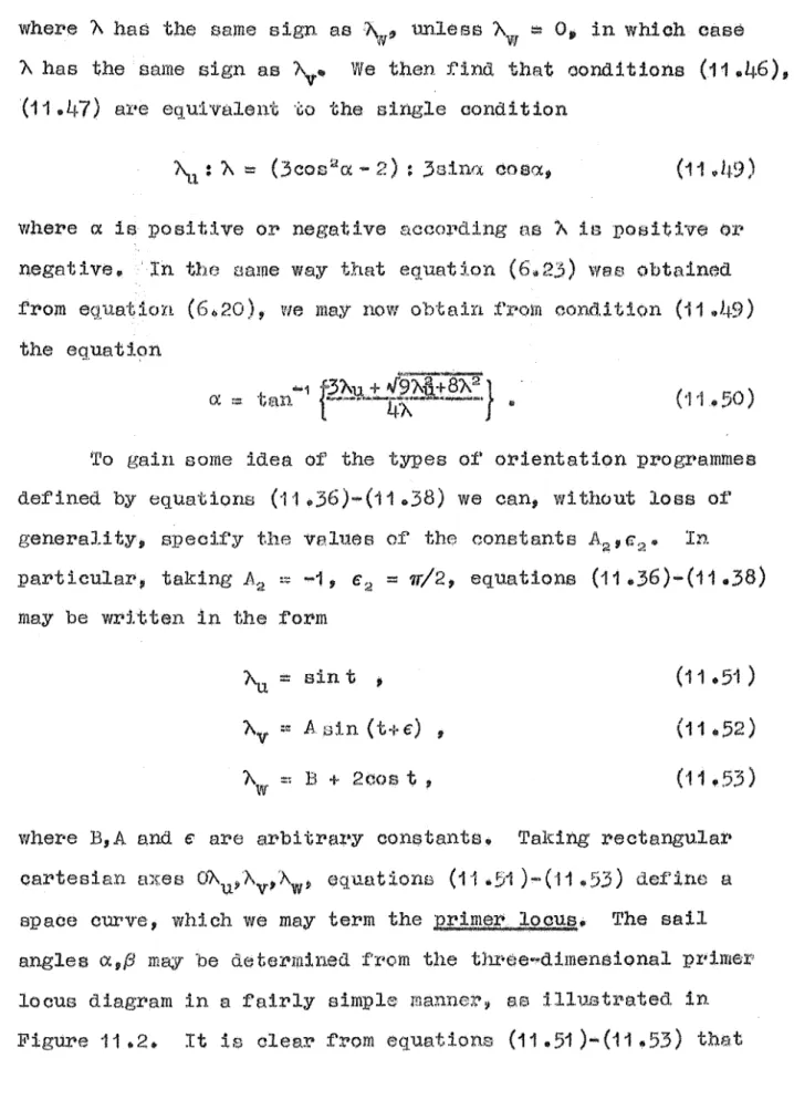
(3 .. 16) a,b,c,cl are constants. 'rhur;; f'rom ions ( 3 .1 2 ) , ( 3 .. 1 5 ) and (3.16) ₁₁ 0 is clotermined according to the ions

use o:e f'amil concept the' imer locus• we may int equat (3.17) pictorially.. Thtus we suppose 'Au, 'Av to be the components of' a vect.o:t• primer vector, so

that es linearly with ct to time, in accordance with ions

(3 .. 15),(3.16) ..

The tip of' the mer• vector moves

a stra line with constant velocity. This line is

called~ the ime1~ locuB and shown in t UB now

resolve the prime:t• vector along axes 0/\ti_/\~ obtained !'rom the axes OAu'Av by l"Otation th:r•ough an 0,.

see that

'A~

=

'AucosB + /\vsinB , (3 .. 1 B) )\; = -'AusinB + 'A..,coc:,() ..

Then, st'tbstj:tut :from equntJon (3.,12) into the quotient of' equations (3 .. 1 B), (3 .. 19) we

'A'

v

that

If' we clef'j.ne thtj (3 by the equation

then equation (3.20) be written

te.n/3

=

2 fJ ..

In , equation (3.. ) will have two solutions :tn. the

interval [ ... 7T/~~, +7T/2] , as indicated. in the f'igure.. One of' ther:Je will be eliminHted by the eondi t:l on ..

ier•ntr•am;: eo:ndi tion iB considered in il in

section 7 vw may decJuce :f'rom the presented there that

fJ is c.itive or• ive 5.ve oP

OJ.)timizing

l~quation (3.. ) is f'amiliaPo~ In J':'act, it is icle:nti with equation ( 2 .. 6). 'I'hc cation is that

e

is r:;o as to maxhrtize force component in the d ction of' the primer ve cto:r·.,

the ion p1•ovi by the We s

condition we may UBe

ded-uot about 0-pr•ogr•amrne to

v1e notice -~hat () o1wnges .Crom -rr/2 to +·rr/2 (o:r;• vice versa), "-u being ive., '.rhis clEmJonstx•ates

fHJlbili a corner be trajec

the co:nrli tio:n :Cor· this is, f':r•om _ions

_{(3.15),(3.16),}

also note tJ:mt, with the possible exception of' a Bingle int dlscontinu.it;y, 0 is either monotonically inCl"'easing or

mono-tonically _{creaE:1ing.. 'J'he general :Co:t•m of the 0-I:n~ogramme is} shown 5.n

The time origin is t _{to be the point at which '"Ay vani} Othe:r- possi'ble gcnel'al progr•ammes m~e obtainable from f 3 .. 3 .. (1) and 3 .. 3 .. (ii) by _{the time axis..}

.M1 t ~ ± co :.l.t

will _{noticed tht"l.t 0 tendB to two 1imi tin1_.; values denoted by}

consist of some section t _{f':t'om the gene:r•al p:r•og:r•amrner3 3(j.)} or {3( ii) taken between two time limi tu tb

While _{3 .. 3., shovts the most}

behaviour of fJ ns a f'unction o:r time, we must also _{aome ecial case:;;..}

will be convenient in th~.s Part to distingu1eh. quantities which

are

to O(i!i ealculated

at

the departure and arrival

terminals by subscripts b and t respectively.

The 0-programme is particularly simple if' the primer locus

B throu.gh the ortgin.. •rhe belu:IViour in thJ.s cam:; is

il:Lustr•atecl :ln

If' direction o:C of~ _int p _i f:J flS by the

ar-:t•ow in !I th.e (:J ste initially ot' a corwtant negative angle

-

~['his s to a constant

po ti ve angle (:J

1 I:HJ P pa.t:H3es thr•oue;h the origin. '.L'he act;ual

magnitude of' the is determined by the gradient the line OP,. ]j'rom equat:i.ons (3,.15), (3 .. 16) we find that the

condi-t pr•imer locus pass throu,gh the ori is a

c1 = 0 ~

It is also possible for primer locus to d(;'lgenerate to a po:tnt.. Thie occurs wh.en a and b both sh. In this case 0

lr~ constB.nt :Cor

In to illustrate above theor-y we will consi<ler a PEJ.r>ti culal"' t ation problem, namely maxhnization of

I,et V(:x:,y) be the gravitatj.onal :potential so that

cr ::;:

-av/. ay ..

""'y

(3. 25) (3.. )

a vehicle o:t' 'l:tn:i.t mass the kinetic e:nert;ry is given by

We may, without loso generality, tial values

at an initial time

t :::=

o ..

The rinal time will then be

..

Denoting the the subGcr t fi we see thB.t the :t'inal net

(3 .. 27)

(3 .. 28)

values by

by

(3 .. 29) Thus we .mHy clef'ine ,J ₁ the pnyof'f' f'unct ion to be minimi , by the equation

.J ::::

..

~:l ince at•e not prescr•ibed.2 we have the bou:ndru•y conditions

the t i 8 f'ol» any the VfJ:t""i

"

=

-

II

:X{ (:'> .. 32)

"

Y:i

...

p;y

'

( 7. .)

..

)

"u ::::::: uf 1

(3.34)

"

= _v1

..

V{

Equations

(3.13)-(3 .. 16),(3 ..

)-(3.35)

lee to determine the constants a,b, c,d., T'he£;e are

,

'b =

-c

=

'llf- ,

d ::::: Vt - gy t! 11

a:nd , f'rom equnt:l.ons ( .. 15L ( .. 16), the pr•imer~ v·ector cornponenta :a.:r:e r':iven by

"' _{"u -}- U t -_:~.

(3 .. 37)

(3~38)

( _{. ) •} "7- )

(3 .. }+0)

(3~41 )

will clearly be thc'!t j:'o:t' I'Jh:i ch ld vanishes. In this case we have

:::::::

=

₀

::md cH.runtions (3 .. liO), (3 ..

4.1 )

combine to give

the p:r•imer vector is constant VJi th Pe ect to t and coincides with the final velocity. Since is no