Progressive Randomization of a Deck of Playing Cards: Experimental Tests and Statistical Analysis of the Riffle Shuffle

(1)

http://www.scirp.org/journal/ojs ISSN Online: 2161-7198

ISSN Print: 2161-718X

DOI: 10.4236/ojs.2019.92020 Apr. 28, 2019 268 Open Journal of Statistics

Progressive Randomization of a Deck of Playing

Cards: Experimental Tests and Statistical

Analysis of the Riffle Shuffle

M. P. Silverman

Department of Physics, Trinity College, Hartford, CT, USA

Abstract

The question of how many shuffles are required to randomize an initially or-dered deck of cards is a problem that has fascinated mathematicians, scien-tists, and the general public. The two principal theoretical approaches to the problem, which differed in how each defined randomness, has led to statisti-cally different threshold numbers of shuffles. This paper reports a compre-hensive experimental analysis of the card randomization problem for the purposes of determining 1) which of the two theoretical approaches made the more accurate prediction, 2) whether different statistical tests yield different threshold numbers of randomizing shuffles, and 3) whether manual or me-chanical shuffling randomizes a deck more effectively for a given number of shuffles. Permutations of 52-card decks, each subjected to sets of 19 succes-sive riffle shuffles executed manually and by an auto-shuffling device were recorded sequentially and analyzed in respect to 1) the theory of runs, 2) rank ordering, 3) serial correlation, 4) theory of rising sequences, and 5) entropy and information theory. Among the outcomes, it was found that: 1) different statistical tests were sensitive to different patterns indicative of residual order; 2) as a consequence, the threshold number of randomizing shuffles could vary widely among tests; 3) in general, manual shuffling randomized a deck better than mechanical shuffling for a given number of shuffles; and 4) the mean number of rising sequences as a function of number of manual shuffles matched very closely the theoretical predictions based on the Gilbert-Shannon-Reed (GSR) model of riffle shuffles, whereas mechanical shuffling resulted in sig-nificantly fewer rising sequences than predicted.

Keywords

Randomization of Cards, Number of Riffle Shuffles, Rising Sequences, GSR Model, Entropy and Information

How to cite this paper: Silverman, M.P. (2019) Progressive Randomization of a Deck of Playing Cards: Experimental Tests and Statistical Analysis of the Riffle Shuffle. Open Journal of Statistics, 9, 268-298. https://doi.org/10.4236/ojs.2019.92020

Received: March 22, 2019 Accepted: April 25, 2019 Published: April 28, 2019

http://creativecommons.org/licenses/by/4.0/

(2)

DOI: 10.4236/ojs.2019.92020 269 Open Journal of Statistics

1. Introduction: The Card Randomization Problem

Proposed solutions to the problem of determining the number of shuffles re-quired to randomize a deck of cards have drawn upon concepts from probability theory, statistics, combinatorial analysis, group theory, and communication theory [1] [2]. The methods employed transcend pure mathematics, and have implications for statistical physics (e.g. random walk; diffusion theory; theory of phase transitions) [3] [4], quantum physics [5], computer science [6] [7], and other fields in which randomly generated data sequences are investigated. Not only mathematicians and scientists, but the general public as well have shown much interest in the card randomization problem, as reported in popular science periodicals and major news media [8] [9] [10] [11]. This paper reports what the author believes to be the most thorough experimental examination to date of the randomization of shuffled cards, using statistical tests previously employed in nuclear physics to search for violations of physical laws by testing different ra-dioactive decay processes for non-randomness [12] [13] [14] [15].

1.1. Background

Probability as a coherent mathematical theory is said to have been “born in the gaming rooms of the seventeenth century” in attempts to solve one or another betting problem [16]. Among the most ancient forms of gambling are card games, which developed initially in Asia but became popular in Europe after the invention of printing [17]. Depending on what one considers a distinct game, experts in the subject estimate the number of card games to be between 1000 and 10,000 [18] [19]. Most card games are conducted under the assumption that the deck in play has been initially randomized. From a practical standpoint, a deck is considered random if players are unable to predict any sequence of cards fol-lowing a revealed card. (Mathematically, there is on average 1 chance in n of guessing correctly the value of any unrevealed card in a deck of n randomly dis-tributed cards).

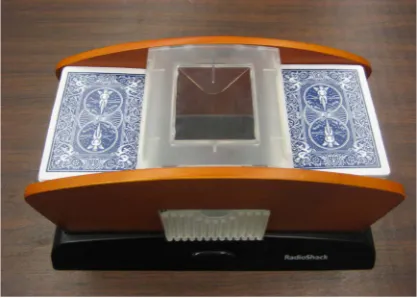
The standard way to mix a deck of cards randomly is to shuffle it, for which purpose the riffle shuffle is perhaps the most widely studied form. To execute a riffle shuffle, one separates (“cuts”) the deck into two piles, then interleaves the cards by dropping them alternately from each pile to reform a single deck. The process can be performed either by hand or mechanically by an auto shuffler, like the device shown in Figure 1 used to acquire some of the data reported in this paper. Clearly, a single riffle shuffle cannot randomize an ordered deck be-cause the order of cards from each pile is maintained. Indeed, in a perfect riffle shuffle of an even-numbered deck, whereby the deck is cut exactly in half and 1 card is dropped alternately from each pile, there would be no randomization at all. Instead, the sequences of cards resulting from a series of perfect riffle shuffles cycle through a fixed number of permutations leading back to the original card order. For example, a pack of 52 cards recycles after only 8 perfect “out-shuffles” (i.e.

(3)

[image:3.595.269.478.72.221.2]

Figure 1. Motor-driven mechanical card shuffler used to generate auto-shuffled card se-quences. Two piles of cards placed as shown are displaced from below by rotating wheels so as to drop sequentially into the central chamber.

where shuffles are not perfect, the order of the cards from each pile is degraded with each successive riffle shuffle.

The central question comprising the card randomization problem is this: How many riffle shuffles are required to randomize a deck of cards? More accurately stated: After how many shuffles can one detect no evidence of non-randomness? Various researchers have studied this question theoretically and arrived at statis-tically different answers, depending on the adopted measure of randomness. In the analysis of Bayer and Diaconis [1], the measure of randomness of the deck is the so-called variation distance (VD) [4] [21] between the probability density

,

n m

Q of n cards shuffled m times and the uniform density Un=1 !n of the permutation group Sn of n distinct objects. In the limit of large n, the VD

analysis predicted that

( )

VD 2

3 log 2

m n ≈ n (1)

shuffles should adequately randomize a deck of n cards. Thus mVD

( )

52 is

about 8 - 9. According to [1], VD quantifies the mean rate at which a gambler could expect to win against a fair house by exploiting any residual pattern of the cards. The researchers also showed that the VD between Qn m, and Un takes

the form

2

1 4 3 2 ,

2

1 e d 0.115

2π

t

n m n

Q U − − t

−∞

− = −

_∫

≈ ₍₂₎ for large n with m given by Equation (1). For complete randomness, the VD would equal 0.

In a numerical analysis by Trefethen and Trefethen [2], the adopted measure of randomness was based on the Shannon entropy of the deck in the sense of in-formation theory [22] [23]. If pj

(

j=1,, !n

)

is the probability of the j

th

permutation of Sn, then the Shannon entropy of the deck is given by !

2 1

log

n

j j

j

H p p

=

(4)

where, by completeness,

!

1

n

j j

p

= =

∑

, (4) and the information associated with the set of probabilities

{ }

pj was defined as

( )

2

log !

n

I = n −H. (5)

According to [2] In in Equation (5) quantifies the rate at which an ideally

competent coder could expect to transmit information if the signals were en-coded in shuffled decks of cards. In the limit of large n, the information theoretic (IT) calculation predicted that

( )

IT log2

m n ≈ n (6)

shuffles should adequately randomize a deck of n cards. Thus mIT

( )

52 is about

5 - 6, in contrast to mVD

( )

52 . The numerically obtained results of [2] were

sub-sequently proved theoretically by another research group [24].

The structure of relation (5) provides a mathematical definition of the word “information” consistent with its general vernacular use. If there is no uncer-tainty in the communication of any n-symbol message based on card sequence, then p_j =1 for each permutation j. In that case H =0 and the information

2

log !

n

I = n is maximum. If, however, every message received is completely

uncertain as to card order, then p_j=1 !n for each permutation j,and therefore,

by use of Equation (4), the information In =0. Alternatively [25], physicists and other scientists usually associate the concept of information with entropy H, Equation (3). The rationale is that the greater the uncertainty (i.e.H) of a mes-sage or physical system, the more information one gains by a binary decision (or measurement) that reduces the uncertainty. In a system with perfect order, H = 0; the outcome of any measurement or decision is completely predictable, and therefore no new information is to be gained. Both definitions of information prove useful later in the paper (Section 3.4).

Although the two analyses [1] and [2] led to statistically different distributions of randomness as a function of shuffle number, they both started from the same mathematical model of shuffling, referred to as the GSR shuffle, named for Gil-bert and Shannon [26] and, independently, for Reeds [27]. The GSR shuffle in-volves the following steps. The deck is cut roughly in half according to a binomi-al distribution in which the probability that a pile contains k out of n cards is

2 n n k

C

− _where

(

!

)

! !

n k

n C

k n k

≡

− (7) is the binomial combinatorial coefficient. The two halves are then riffled togeth-er such that the probability of a card being dropped from a pile is proportional to the number of cards in the pile.

1.2. Outline of Paper

(5)

extensive list of references that survey the development of the problem, of which virtually all papers are theoretical analyses or numerical modeling by computer simulation, can be found in [28]. To the best of the author’s knowledge, there has been no comprehensive, systematic experimental examination of the card ordering and patterns produced by manual shuffling to test whether the results conform to the GSR model or support the published theoretical predictions.

This paper reports on an extensive set of tests by which was measured the progression toward randomness of card sequences produced in multiple riffle shuffles manually and, for comparison, by a mechanical auto shuffler.

The basic theory and experimental outcomes of the following measures of randomness are discussed in Section 2: 1) runs with respect to the mean, 2) runs up/down, 3) rank ordering, 4) serial correlation (lag 1), and 5) theory of rising sequences.

Analysis of the data by information theory is discussed in Section 3. Conclusions are presented in Section 4.

2. Experiment and Statistical Tests

Experiments were undertaken to examine the permutations of card order in a deck of n = 52 cards as a function of shuffle number m for m=0,1,,M

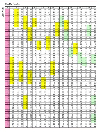
im-plemented N times. For the experiments reported here, the number of shuffles per set is M = 19 and the number of sets is N = 12. In addition to manual shuffles, the experiments were also carried out with the mechanical auto shuffler of Figure 1. The cards used in manual shuffling were not new, but had already been flexed many times previously in play and were therefore more pliant than stiff new cards. This requirement was irrelevant for auto shuffling, since the cards were flat, not flexed, when distributed by the machine into two piles. A sample of the data obtained from one set of M shuffles is shown in Table 1.

The experiment began with an ordered deck (column m = 0, highlighted in red), with card values increasing from 1 (top card) to 52 (bottom card). Permu-tations of card order for each shuffle m=1, 2,,M are recorded sequentially

in columns from left to right. A cursory examination of the table immediately reveals patterns of ascending sequences (highlighted in yellow) and descending sequences (highlighted in green) that extend across all the columns. Each of the

N sets of card shuffles was subject to a variety of statistical tests to quantify the non-randomness of the permuted orderings indicated by these and other pat-terns.

2.1. Theory of Runs

A run is defined as a succession of similar events preceded and succeeded by a different event. For example, the sequence of 12 symbols

b b a a a b b b a b a b

(6)

[image:6.595.211.537.85.527.2]

Table 1. Card sequences after 19 riffle shuffles of an initially ordered deck.

2 runs of of length 1 2 runs of of length 1 1 run of of length 2 1 run of of length 3 1 run of of length 3

a b b a b

(8)

or a total of 7 runs. If a sequence is random, then all permutations of symbol or-der should have the same probability of occurrence. From this invariance prin-ciple, as applied to a sequence containing na symbols of type a, nb symbols of

type b, and n=na+nb symbols in all, it can be deduced that [29]:

• the mean number of runs of a of length precisely k (where k≥1) is

(

)(

)

(

)

! 1 1 !

! !

a b b

ka

a

n n n n k

r

n k n

+ − −

=

(7)

• _{the mean number of runs of} a of length k or greater (i.e. inclusive runs) is

(

)(

)

(

)

! 1 !

! !

a b

ka

a

n n n k

R

n k n

+ −

=

− (10)

• _{the mean number of total runs of both kinds is}

1 1

2 _a _b

a b

n n n

R R R

n

+

= + = . (11) Expressions for rkb, Rkb follow, mutatis mutandis, from Equation (9) and

Eq-uation (10). Proofs of these expressions are given in [30] [31].

Two methods were employed in this paper to generate runs of binary symbols from the experimentally recorded sequences of digital card values.

2.1.1. Target Runs

The card value xi

(

i=1,,n

)

at location i in the sequence resulting from a

particular shuffle is compared with a target value X, here taken to be the mean

1 1 26.5 n i i X x n =

=

∑

→ ₍₁₂₎

which reduces as shown for the case n=52 with set of card values

{

x=1, 2,, 52

}

. If x_i< X, the symbol 0 is assigned to location i; if xi >X , the

symbol 1 is assigned to location i. Because the set

{ }

xi is comprised of integers,

the event xi = X cannot occur. Moreover, the set is equally partitioned:

1 0

1 2

n =n = n,

and the mean number of total runs, Equation (11), reduces to

mean

2 27 2

n

R = + → (13)

where the numerical value again applies to the case of n=52.

The associated variance (with corresponding standard deviation) is given by

[29] 2 mean mean 1 1 1

4 1 4

3.57 n n n σ σ −   ≈ _ − _≈ −   → (14)

with numerical evaluation for n=52. It can also be shown that the test statistic

( )

mean mean mean 0,1 R R z N σ −

= → ₍₁₅₎ for the observed total number of runs is approximately Gaussian for sufficiently large n. The symbol N

( )

0,1 designates the standard normal distribution of

mean 0 and variance 1.

As an example, consider the 10-card decimal sequence generated by a uniform random number generator (RNG) over the integer range (1 ... 52):

{

29 47 45 32 6 34 44 36 38 5

}

(8)

The resulting binary series with target taken to be the mean (12) is then

{

}

mean 1 1 1 1 0 1 1 1 1 0

y = (17)

which comprises the following set of target runs 2 runs of 0 of length 1

2 runs of 1 of length 4 (18) for a total of 4 runs with respect to the mean.

For a long equipartitioned sequence (n1=n01), the contribution of runs at

the start or end of a sequence becomes negligible compared with the number of runs within the sequence, and Equation (9) and Equation (10) may be approx-imated as follows [32]

2

2 ka k

n

r ≈ ₊ (19)

1

2 ka k

n

R ≈ ₊ . (20)

Equation (19) and Equation (20) are illustrative of the general exact relation

( 1)

ka ka k a

r =R −R ₊ (21)

that follows from the definitions of rka and Rka. 2.1.2. Runs Up/Down (or Difference Runs)

An alternative method of generating sequences of binary symbols that provides an independent test for non-random symbol patterns is to calculate sequential differences of the card values as follows

(

)

1 1, , 1

j j j

y =x+ −x j=  n− (22)

and assign 1 to a positive difference

(

y_j >0

)

and 0 to a negative difference

(

y_j<0

)

. Since there is no repeating integer in the set

{ }

x_i , the value y_j=0

cannot occur. Thus, a sequence of 52 card values is transformed into a sequence of 51 binary difference values.

For example, consider again the 10-card decimal sequence (16):

{

29 47 45 32 6 34 44 36 38 5

}

x= . (23)

The resulting binary difference series is then

{

}

diff 1 0 0 0 1 1 0 1 0

y = (24)

which comprises the following set of up/down runs 2 runs of 1 of length 1 2 runs of 0 of length 1 1 run of 1 of length 2 1 run of 0 of length 3

(25)

for a total of 6 up/down runs.

(9)

com-DOI: 10.4236/ojs.2019.92020 276 Open Journal of Statistics

pletely different outcomes of up/down and target runs tests. Thus, the two kinds of runs procedures independently test the same decimal sequence for different symbol patterns.

A major difference between the target runs and the up/down runs is that riates in the former (e.g. series (17)) are realizations of Bernoulli random va-riables (i.e. the probability of occurrence is the same irrespective of location within the series), whereas the variates in the latter (e.g. series (24)) are not. For up/down runs, the greater the length of a run, the less probable is the occurrence of yet another symbol of the same kind. The expectation values of up/down runs, therefore, differ from those of target runs. Instead, the expressions correspond-ing to (9)-(11) are [29]:

• _{the mean number of up and down runs of length precisely}_k_(where k≤ −n 2)

is

(

23 !

)

(

2 3 1

) (

3 3 2 4

)

k

r n k k k k k

k  

= _ + + − + − − _

+ (26)

• _{the mean number of up and down runs of length}_k_{or greater (where} k≤ −n 1)

is

(

22 !

) (

1

)

(

2 1

)

k

R n k k k

k  

= _ + − + − _

+ (27)

• _{the mean total number of up and down runs is}

(

)

u/d

1

2 1 34.33

3

R = n− → (28)

with associated variance and standard deviation

(

)

2 u/d u/d

1

16 29

90 2.99

n σ

σ

= −

→ (29) Evaluations in Equation (28) and Equation (29) pertain to n=52.The statistic

( )

u/d u/d

u/d

0,1 R R

z N

σ

−

= → (30) is again approximately normally distributed.

2.1.3. Runs Tests of Shuffled Cards

The total numbers of target runs and up/down runs were calculated as a func-tion of shuffle number for each of the N sets of M shuffles, such as exemplified

by Table 1. Note that the ascending sequences (yellow) and descending

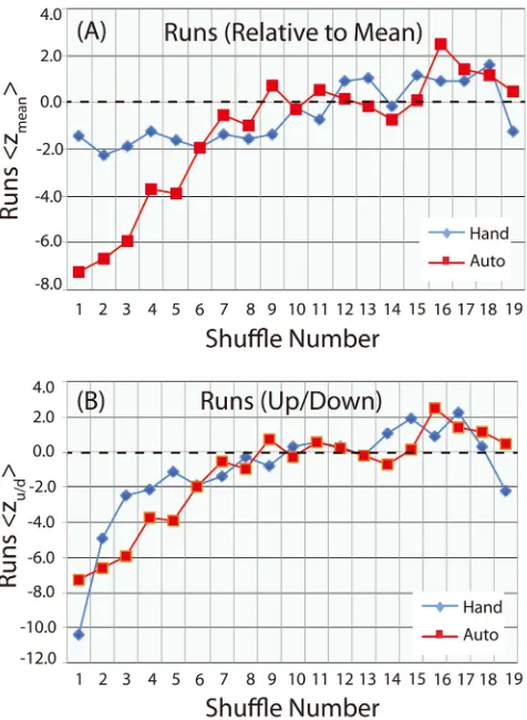
se-quences (green) respectively correspond to examples of up and down runs. The mean of the N values for each shuffle number was then calculated and converted to standard normal forms expressed by (15) and (30). Figure 2 shows plots of

mean

z in frame A and zu/d in frame B as a function of shuffle number.

(10)

[image:10.595.253.491.71.396.2]

Figure 2. Runs statistics as a function of number of shuffles obtained by hand (blue curve) and machine (red curve) for (A) runs relative to the mean and (B) runs up/down. Values within about ±1 standard deviation of the expected value 0 can be taken to indicate a randomly ordered deck.

statistic z ≤1. Also, for shuffle numbers below threshold, decks shuffled by

hand (blue curves) manifested greater disorder than decks mixed by the auto shuffler (red curves).

2.2. Rank Correlation (or Rank Order)

The Spearman rank correlation coefficient rS is a nonparametric measure of

the association between two random variables X and Y as defined by their rank order in a sequence of n pairs [33]

(

)

2

1

S ₂

6 1

1

n

i i

D r

n n

= = −

−

∑

(31)

in which

( ) ( )

i i i

D =r x −r y (32)

is the difference between the ranks assigned to samples xi and yi (When a

(11)

DOI: 10.4236/ojs.2019.92020 278 Open Journal of Statistics X)).

Values of rS range from −1 to +1, respectively signifying perfect

an-ti-correlation (i.e. reverse rankings) and perfect correlation. It is 2 S

r , however,

rather than rS, that has a statistical interpretation;

2 S

r is a measure of the

va-riability of the data attributable to the correlation between variables X and Y [34]. Thus a relatively high correlation coefficient such as rS=0.7, means that only

49% of the variability is accounted for by the association between X and Y. For independent variables (and therefore uncorrelated ranks), the expectation value and variance are respectively

S 0

r = (33)

S 2 1 1 r n σ =

− , (34) and the test statistic

( )

S

S S

rank S 1 0,1

r

r r

z r n N

σ

−

= = − → (35)

follows a standard normal distribution to good approximation [35].

Applied to the shuffling of cards, the variable Y signifies the initial card se-quence

{ }

yi m=0=

{

1, 2,, 52

}

and variable X signifies the card sequence

{ } {

xi m= x1,,xn

}

of the m

th_{shuffle. Since the face values of the cards range}

from 1 to 52, the rank of a card is equal to its face value. Therefore an equivalent, but simpler, way to perform the rank correlation test is to calculate the cross correlation of ranks

( ) ( )

( )

rank

1 1

n n

j j j

j j

C r x r y jr x

= =

≡

∑

=

∑

₍₃₆₎

where the second equality in (36) pertains specifically to the sequence of cards in a deck of n cards. The expectation value and variance of Crank are respectively

(

)

2 rank

1

1 36517 4

C = n n+ → (37)

(

) (

)

2

2 2 rank rank 1 1 1 444 1640.15

n n n

σ σ

= − +

→ (38) with numerical evaluations for n=52. The test statistic

rank rank rank rank C C z σ −

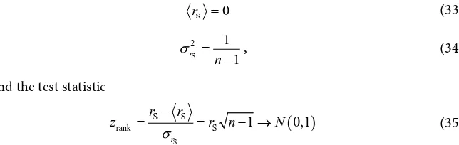
[image:11.595.213.535.212.314.2]

= ₍₃₉₎ can be shown to be identical to that of Equation (35) [33].

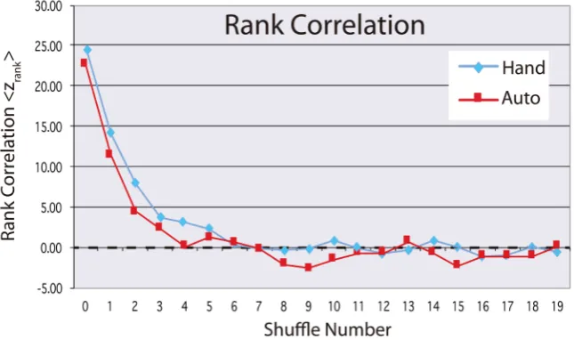
Figure 3 shows a plot of zrank , i.e. Equation (35) or (39) averaged over the

N sets of data for each shuffle number m for both manual (blue) and auto (red) shuffled cards. The correlation between the card sequence of the mth_{shuffle and}

the initial card sequence (m = 0) is interpreted as statistically 0 (i.e. for zrank ≤1)

(12)

[image:12.595.213.536.76.267.2]

Figure 3. Rank ordering statistics as a function of shuffle number for manually (blue) and auto (red) shuffled cards. Values within about ±1 standard deviation of the expected val-ue 0 can be taken to indicate a randomly ordered deck.

2.3. Serial Correlation Lag-1

Serial correlation refers to the relationship between elements of the same series separated by a fixed interval. Given a sequence of elements

{ }

xj for

1, 2, ,

j=  n, the serial correlation coefficient lag-k is defined by [36]

2 1 1 2 2 1 1 1 1 n n

j j k j

j j

k

n n

j j

x x x

n x x n ρ + = = = =   −     =   −    

∑

(40)

where xj k+ is to be replaced by xj k n+ − for all values of j such that j+ >k n.

For the purpose of testing correlations in card order following shuffling, the most useful serial coefficient is ρ1, which measures the correlations between

pairs of consecutive cards. It can be shown, however, that a test based upon the simpler statistic [37]

1 1

1 n

j j j

c x x+

=

∑

₍₄₁₎

is equivalent to a test based on ρ1. The mean and variance of c1 are given by

the following expressions [36] [37]

2 1 2 1 1 S S c n − =

− (42)

(

)(

)

1

4 2 2

2

2 2 4 1 4 1 2 4 1 3 2 2 4

1 1 2

c

S S S S S S S

S S

n n n

σ = − + − + + −

− − − (43)

where 1 n k k j j S x =

(13)

For large n, the statistic

1

1 1

serial c

c c

z

σ

−

= (45)

follows a standard normal distribution to good approximation.

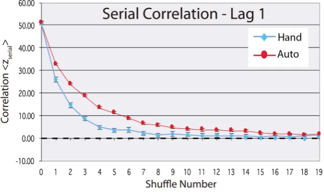
Figure 4 shows a plot of zserial , i.e. Equation (45) averaged over the N sets

of data for each shuffle number m for both manually (blue) and auto (red) shuf-fled cards. The correlation between the card sequence of the mth_{shuffle and the}

initial card sequence (m = 0) is interpreted as statistically 0 (i.e. for zserial ≤1)

starting at about m = 8 (manual) and m = 16 (auto).

2.4. Rising Sequences

A rising sequence, as defined in [1], is a maximal consecutively increasing subset of an arrangement of cards. For example, consider a hand of 8 cards with the sequence of face values: 1 6 2 3 7 8 4 5. By displaying the cards in the following way

{ }

6 7 8

1 2 3 4 5

i

x =  _

  (46) one sees that the hand consists of two rising sequences (1,2,3,4,5) and (6,7,8) in-terleaved together. Successive riffle shuffles tend to double the number of rising sequences up to a maximum number of 1

(

1

)

2 n+ in the limit of an infinite number of shuffles. Note that a rising sequence is different from an ascending sequence (i.e. a run up): 1) The elements of a run up merely ascend, but do not have to increment successively; 2) The elements of a rising sequence do not have to be contiguous (as in a run), but can be separated by other elements.

[image:13.595.214.535.495.685.2]

It is shown in [1] that the probability of a particular permutation following a

(14)

riffle shuffle depends only on the deck size n and the number r of rising se-quences in the permutation. Specifically, the probability that the mth_{riffle shuffle}

of an ordered deck has r rising sequences is

( )

2

,

1 2

n r n m mn n

Q r = C + − . (47)

The mean number of rising sequences in the permutation following m shuffles is then given by

( )

, ,

1 n

n m n n m

r

r rE r Q r

=

∑

(48) where the Eulerian number [38]

( )

1

( )

1

r

r j _n _n

n r j

n

E r j C

+ ₋

+ − =

=

∑

− ₍₄₉₎

is the number of permutations containing r rising sequences. Substitution of Equation (49) into Equation (48) leads to the simpler expression [39]

2 1 , 1 1 2 2 m m n

n m mn

r n r r − = +

= −

∑

_{. (50)} The sum of powers of an uninterrupted sequence of positive integers, such as contained in expression (50), is given by Faulhaber’s formula [40]

(

)

1

1 2

1 !

1 2 ! 1 !

n

R n

n n k n k

r k

B

R n

r R R

n k n k

+

− +

= =

= + +

+ − +

∑

(51)

in which Bk is a Bernoulli number, defined by the generating function [41]

( )

(

)

0

coth 2

2 1 !

e 1 k k t k B t t t t k ∞ = − = =

−

∑

(52)

and given explicitly by

( ) ( )

( )

0 1 / 2 1 1 2

0 3, 5, 7,

1 2π 2 ! 2, 4, 6,

k k k

B B

k B

k ζ k k

− = = − =  =  − − =    (53)

where the Riemann zeta function is defined by (Ref. [41], pp. 329-330)

( )

1 p

k

p k

ζ ∞ −

=

∑

. (54) In the limit R→ ∞, the sum in the right side of Equation (51) becomes

neg-ligible, and therefore

1 1 1 lim 1 2 n R n n R r R r R n +

→∞ =

∑

→ + − . (55)

Substitution of relation (55) into (50) with R=2m leads to the asymptotic

number of rising sequences after an infinite number of riffle shuffles

(

)

, ,

1

lim 1 26.5

2

n m n

(15)

as stated without proof at the start of this section. The numerical evaluation per-tains to a deck with n = 52.

The mean-square number of rising sequences for m shuffles can be calculated numerically from Equation (47) and Equation (49)

( )

2 2

, ,

1 n

n m n n m

r

r r E r Q r

=

∑

₍₅₇₎

from which follows, also numerically, the theoretical (i.e. population) variance

2

2 2

, , ,

n m rn m rn m

σ

= − _{. (58)}

[image:15.595.203.538.335.743.2]

The author was unable to determine an analytical closed-form expression for (57) or (58).

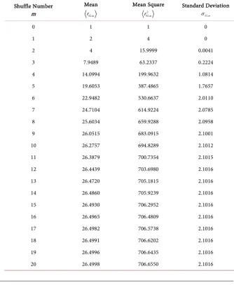
Table 2 summarizes the relevant statistics of rising sequences based on the GSR model as a function of shuffle number m for a deck of 52 cards. It is seen that about 13 shuffles are required to achieve the asymptotic result of Equation (56). In Figure 5 the theoretically predicted mean number of rising sequences Table 2. Statistics of Rising Sequences in a deck of 52 cards.

Shuffle Number m

Mean

52,m

r

Mean Square 2 52,m

r

Standard Deviation 52,m

σ

0 1 1 0

1 2 4 0

2 4 15.9999 0.0041

3 7.9489 63.2337 0.2224

4 14.0994 199.9632 1.0814

5 19.6053 387.4865 1.7657

6 22.9482 530.6637 2.0110

7 24.7104 614.9224 2.0785

8 25.6034 659.9288 2.0958

9 26.0515 683.0915 2.1001

10 26.2757 694.8289 2.1012

11 26.3879 700.7354 2.1015

12 26.4439 703.6980 2.1016

13 26.4720 705.1815 2.1016

14 26.4860 705.9239 2.1016

15 26.4930 706.2952 2.1016

16 26.4965 706.4809 2.1016

17 26.4982 706.5738 2.1016

18 26.4991 706.6202 2.1016

19 26.4996 706.6435 2.1016

(16)

[image:16.595.241.509.72.277.2]

Figure 5. Mean number of rising sequences for manual (blue) and auto (burgundy) shuf-fling as a function of shuffle number. Superposed is the theoretical (red) mean and un-certainty (±1 standard deviation) predicted for the GSR model of the riffle shuffle.

,

n m

r is compared with the observed numbers obtained by manually and auto

shuffled cards averaged over the N data sets. Several features are to be noted: • _{In contrast to the statistical behavior graphically displayed in preceding}

fig-ures which showed gradual randomization with increasing shuffle number m, the mean number of rising sequences underwent a relatively abrupt transi-tion from a non-random state to the asymptotically random state at a thre-shold shuffle number m = 7 or 8 for manual shuffles and m = 11 or 12 for auto shuffles.

• _For m<4, the three curves (theory, manual shuffle, auto shuffle) yielded virtually identical results.

For m≥5, the rising sequences due to manual shuffling were statistically coincident with theoretical predictions, whereas shuffling by machine yielded too few rising sequences at each shuffle number up to the asymptotic number

A 13

m ≈ . This feature suggests one can randomize a deck better by shuffling it

manually than by use of a mechanical auto shuffling device like that in Figure 1.

3. Entropy and Information Loss

3.1. Entropy of Rising Sequences

As discussed briefly in Section 1.1, the Shannon entropy of a set of n symbols is given by

!

2 1

log

n

j j

j

H p p

=

= −

∑

₍₅₉₎

where pj

(

j=1,, !n

)

is the probability of the j

th_{permutation of the} _n_!

(17)

(Boltzmann’s constant kB), the Shannon entropy, usually expressed in terms of

natural logarithms, provides the basis for deriving the partition function—and therefore all the thermodynamic potentials—of equilibrium statistical mechanics

[42]. From a physicist’s perspective, H is a universal measure of the disorder of a system, maximum randomization occurring when all pj are equal. For a

maximally randomized system of n = 52 symbols, H =log2n!≈225.58 bits.

Although Equation (59) yields the entropy of a sequence of n distinct uncor-related symbols, it does not predict the entropy correctly when the permutations are constrained by rules that create correlations among the symbols. To chart the increasing disorder in a system of n cards as a function of the number m of riffle shuffles one can calculate the entropy of all configurations of a fixed number r of rising sequences and then sum that entropy over the total number of rising se-quences produced in the shuffle. In this case, the relevant probability function is

( )

, ,

n m n n m

p r =E r Q r (60)

with expressions for En

( )

r and Qn m,

( )

r given respectively by Equation (49)

and Equation (47). This procedure leads to a much lower maximum entropy than Equation (59) because it respects the constraints imposed on possible or-derings by the physical mechanism of the riffle shuffle. It has been shown that the possible outcomes to m riffle shuffles of an ordered deck are equivalent to the outcomes of cutting a deck into 2m packets and interleaving the cards from

[image:17.595.245.506.447.654.2]

different packets in such a way that the cards from each packet maintain their relative order among themselves [1] [39].

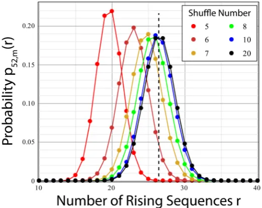
Figure 6 shows the variation in pn m,

( )

r as a function of r for various

in-creasing values of m. In the limit of large m, which for all practical purposes

(18)

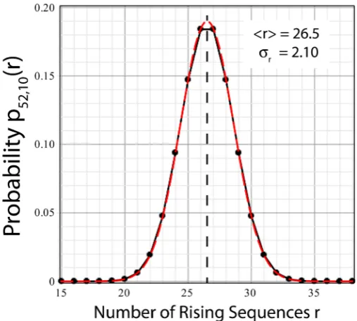
starts at about m = 10 (blue curve), the distribution over r is a nearly perfect Gaussian function, shown by the dashed red curve in Figure 7, centered on the asymptotic number of rising shuffles, Equation (56), marked in the figures by a vertical black dashed line. The width (i.e. standard deviation) of the Gaussian is approximately 2.10, as given in Table 2 for m≥9.

The entropy of a deck of n cards as a function of shuffle number m, calculated from the probability distribution (60), takes the form

( )

, , 2 ,

0

log

n

n m n m n m

r

H p r p r

=

= −

∑

(61) and is plotted in Figure 8 for decks of size n = 14, 26, and 52. The transition between initial complete order Hn,0=0 and maximum disorder is sharp like a

phase transition, such as exhibited by the mean number of rising sequence in

Figure 5. For n = 52, the maximum entropy H52,m≥7≈3.12 bits is reached by

the 7th_shuffle.

3.2. Conditional Entropy

Equation (61) yields the total entropy of a card deck subject to m riffle shuffles. However, it does not provide information on the randomization of specific card associations, which is the kind of information that serious players might rely on for advantage in competition or gambling. For this purpose, the conditional en-tropy of pairs of ordered sequences was determined experimentally.

Let X and Y be two discrete random variables spanning the same range of n

sequential integers (i=1, 2,,n) with joint probability function pXY

(

x y,

)

and

[image:18.595.249.503.452.680.2]

marginal probability functions

(19)

[image:19.595.236.511.67.311.2]

Figure 8. Shannon Entropy (in bits) of the card sequences arising from m shuffles of an ordered deck of n cards for n = 14 (green), 26 (blue), 52 (red). The entropy function is discrete; connecting lines serve only to facilitate visualization.

( )

(

)

( )

(

)

1

, ,

n

X XY

y

n

Y XY

x

p x p x y

p y p x y

=

= =

=

∑

(62)

each satisfying the completeness relation. The entropy (mean uncertainty) in re-ceipt of n transmitted symbols

{ }

xi or

{ }

yi is

( )

2 1

log log

n

X X

x n

Y Y

y

H X p x p x

H Y p y p y

=

= = −

= −

∑

(63)

The conditional entropy of the sequence

{ }

xi , given that the sequence

{ }

yi

is known, is defined by [43]

(

)

|

( )

2 |

( )

1

log

n

X Y X Y Y

x

H X Y p x y p x y p y

=

= −

∑

_{, (64)}

where the condition probability pX Y|

( )

x y is

( )

(

)

( )

| ,

X Y XY Y

p x y = p x y p y . (65)

(See also Ref. [22], pp 52-53.) The joint entropy of X and Y is then given by

(

,

)

( )

(

)

( )

(

)

H X Y =H X +H Y X =H Y +H X Y . (66)

(20)

[ ]XY

( )

(

)

H ≡H X −H X Y (67)

which is the decrease in entropy of the events X when it is known that events Y

have occurred. Given the preceding interpretation, the function expressed by Equation (67) is taken to represent the information provided by knowledge of the events Y [43].

In the analysis of permuted card sequences in the following two sections, the information function H[ ]XY is one of the important quantities to be deduced

experimentally. Substitution into Equation (67) of the conditional probability

(

)

H X Y from Equation (66) leads to the symmetric relation

[ ]XY

( )

H =H X +H Y −H XY (68)

which is particularly useful for calculation.

3.3. Entropy of Sequences of Card Pairs: Theoretical

To apply the preceding concepts to riffle shuffles, the experimental sequences of digital card values are transformed into two sets of binary values by the follow-ing procedure, schematically shown in Figure 9.

• _{Given a decimal sequence of card values}

{ }

xi for i=1, 2,,n, create the

binary sequence

{ }

bj for j=1, 2,,n−1 defined by 1

1 if 1 0 otherwise

j j

j

x x

b =  + − =

 (69)

• _{Transform the set}

{ }

b_j into the set

{ }

c_k k=1, 2,,n−2, where

1

1 2

k k k

c =b+ − b . (70)

[image:20.595.203.542.288.447.2] [image:20.595.236.510.493.648.2]

Transformation (69) generates a binary sequence of 1’s and 0’s, in which the symbol 1 signifies a pair of cards in numerical order (e.g. 4,5). Transformation

Figure 9. Schematic of procedure for transformation of digital sequence

{ }

xi into

bi-nary sequence

{ }

bj and then into quaternary sequence

{ }

ck from which the pair

(21)

(70) converts the binary sequence into a sequence of four values 1, 0, and 1 2

[image:21.595.208.542.93.397.2]

± _.

Figure 9 illustrates the significance of the four symbols: Panel A: 1

2

c= + signifies that a 1 follows a 1.

Panel B: 1 2

c= − signifies that a 0 follows a 1.

Panel C: c=1 signifies that a 1 follows a 0. Panel D: c=0 signifies that a 0 follows a 0.

Given the set

{ }

ck , the following four pair-association statistics

( )

2

( )

0 1 0, 0 n k k

n I c

−

=

∑

(71)

( )

2

( )

1 1 0,1 n k k

n I c

−

=

∑

(72)

( )

1

( )

2 2 1 1, 0 n k k

n I c

−

− =

=

∑

(73)

( )

1

( )

2 2 1 1,1 n k k

n I c

−

=

∑

_{, (74)}

in which

( )

1 0 k k k c I c c α

α

=  =  _≠

 (75)

count the number of events of the kinds represented respectively by panels A, B,

C, D. To summarize, the statistic n

(

α β,

)

is the number of events of symbol

α

_{followed by symbol} β, where both symbols can take on values of 0 or 1. The statistics n

(

α β

,

)

satisfy the sum rule

(

)

0,1 0,1

, 2 50

n n α β α β = = = − →

∑

(76)

evaluated numerically above for a deck of n = 52 cards.

In this information theoretic analysis, it is useful to think of the

α

_symbols

as the realizations of a “message” variable A that represents a received signal of 1’s and 0’s, whereas the β symbols are the realizations of a following “predic-tion” variable B that represents a predicted signal of 1’s and 0’s. For each succes-sive shuffle of the deck, the set of conditional probabilities p

(

β α

)

determines

the conditional entropy H B A

( )

, which is the uncertainty in predicting B given

knowledge of A.

It is straightforward to show that the conditional probabilities p

(

β α

)

can

be estimated from the pair association statistics (71)-(74) as follows

( )

_{( ) ( )}

( )

0, 0 0 0

0, 0 0,1

n p

n n

=

+ (77)

( )

_{( ) ( )}

( )

0,1 1 0

0, 0 0,1

n p

n n

=

(22)

( )

_{( ) ( )}

( )

1, 0

0 1

1, 0 1,1 n

p

n n

=

+ (79)

( )

_{( ) ( )}

( )

1,1 1 1

1, 0 1,1 n p

n n

=

+ (80) in the limit of a sufficiently large number of sets of shuffles. Note that the order of symbols in the argument of p

(

β α

)

signifies that event

α

precedes event

β, which is the reverse of the order of symbols in the argument of n

(

α β,

)

.

Regrettably, this potential for confusion is the price required to maintain con-ventional statistical notation.

The a priori probabilities pA

( )

α of a received symbol

α

are given by

( )

(

)

0,1 1 , 2 A p n n β

α α β

= =

−

∑

, (81)

or explicitly

( )

0

( ) ( )

0, 0 0,1 ,

( )

1

( ) ( )

1, 0 1,1

2 2

A A

n n n n

p p

n n

+ +

= =

− − . (82)

Similarly, the a priori probabilities pB

( )

β ofapredicted symbol β are

( )

(

)

0,1 1 , 2 B p n n α

β α β

= =

−

∑

, (83)

or explicitly

( )

0

( ) ( )

0, 0 1, 0 ,

( )

1

( ) ( )

0,1 1,1

2 2

B B

n n n n

p p

n n

+ +

= =

− − . (84)

The joint probability pAB

(

α β,

)

of a received symbol

α

and predicted

sym-bol β is given by

(

,

)

( )

(

,

)

2

AB A

n

p p p

n

α β

α β = α β α =

− (85)

where the second equality follows from combining relations (82) and (77)-(80). Given the probability functions constructed above, the a priori entropies of the received (A) and predicted (B) signals are

( )

2

( )

0,1

log

A A

H A p p

α

α α

=

= −

∑

₍₈₆₎

( )

2

( )

0,1

log

B B

H B p p

β

β β

=

= −

∑

₍₈₇₎

and the total entropy of A and B is

( )

(

)

2

(

)

1,0 1,0

, log ,

AB AB

H AB p p

α β

α β α β

= =

= −

∑

_{. (88)}

The information, or decrease in uncertainty of values of B as a result of knowing values of A, is then given by Equation (68)

[ ]BA

( )

H =H B −H B A =H A +H B −H AB . (89)

(23)

physics, where natural logarithms are usually used rather than logarithms to base 2, entropy and information are in units of nats.

3.4. Entropy of Sequences of Card Pairs: Experimental

An experiment was performed in which an initially ordered deck of n = 52 cards was subject to N = 11 sets of M = 19 riffle shuffles per set implemented by the auto shuffler in Figure 1, thereby generating M columns of card permutations for each set such as illustrated in Table 1. The cards were shuffled mechanically, rather than manually, so that the riffle shuffles would be executed as uniformly as possible. The pair association numbers n

(

α β,

)

for each of the M shuffles

were then averaged over the N sets to yield the mean numbers of pair associa-tions summarized in Table 3 and plotted in Figure 10 as a function of shuffle number m.

For a completely ordered deck prior to shuffling (m = 0), there are n− =2 50 occurrences of α =1 followed by β=1, as shown by the plot of n

( )

1,1 (red

[image:23.595.210.539.362.733.2]

curve) in Figure 10. This number drops rapidly with increasing shuffle number, becoming effectively 0 by about m≈8. Correspondingly, the occurrence of α =0

Table 3. Mean pair association numbers for a 52-Card Deck.

Shuffle Number m n( )0, 0 n( )0,1 n( )1, 0 n( )1,1

0 0.00 0.00 0.00 50.00

1 5.82 12.00 12.27 19.91

2 14.27 11.91 12.36 11.45

3 20.91 10.64 11.09 7.36

4 26.64 10.27 10.27 2.82

5 30.27 8.91 8.91 1.91

6 34.00 7.55 7.27 1.18

7 38.36 5.36 5.36 0.91

8 39.18 5.18 5.27 0.36

9 41.00 4.45 4.36 0.18

10 42.91 3.45 3.45 0.18

11 43.55 3.00 3.09 0.36

12 43.64 3.00 3.00 0.36

13 43.82 3.00 3.00 0.18

14 44.00 2.91 2.91 0.18

15 46.00 2.00 2.00 0.00

16 46.91 1.55 1.55 0.00

17 46.55 1.73 1.73 0.00

18 47.64 1.18 1.18 0.00

(24)

[image:24.595.251.504.66.286.2]

Figure 10. Pair association numbers n

(

α β,

)

as a function of number of auto-shuffles.

Symbols 1 and 0 respectively represent an ordered and non-ordered two-card sequence. Thus n

( )

1,1 = number of 2 ordered pairs (e.g. 1,2; 2,3) (red); n

( )

0,0 = number of 2 non-ordered pairs (e.g. 2,1; 3,5) (blue); n

( )

1, 0 = number of non-ordered pairs follow-ing an ordered pair (e.g. 1,2; 3,5) (orange); n

( )

0,1 = number of ordered pairs following a non-ordered pair (e.g. 3,5; 1,2) (green). Black squares mark the actual points; colored connecting lines merely facilitate viewing.

followed by β =0 rises rapidly with increasing m, approaching ≈48, as shown

by the plot of n

( )

0, 0 (blue curve). The plots of n

( )

0,1 (green curve) and

( )

1, 0

n (orange curve), which start at 0 and then fall off gradually from a

max-imum of about 12 at m = 1, are virtually indistinguishable.

The conditional probabilities p

(

β α

)

, deduced from the pair-association

statistics by means of Equations (77)-(80), are plotted as a function of m in Fig-ure 11. In each panel, the conditional probabilities satisfy the completeness rela-tion

( )

0,1

1

p

β=

β α

=

∑

(90)

for α=0,1.

The plots in panel A, which show the conditional probabilities of prediction variable β given received variable α =0, begin at m = 1 because there is no event 0 in a completely ordered deck (m = 0). As the shuffle number m increases, the number of ordered pairs decreases, and p

( )

0 0 approaches 1 while p

( )

1 0

approaches 0. In panel B, the probabilities are conditioned on a received variable 1. As the number of 0 events increase with m, it follows again that p

( )

0 1

ap-proaches 1 and p

( )

1 1 approaches 0. For a gambler or competitive player, the

probability p

( )

1 1 is particularly useful, since it quantifies the chance of a third

(25)

[image:25.595.265.478.72.395.2]

Figure 11. Conditional probabilities p

(

β α

)

as a function of shuffle number for 11

au-to-shuffled sets, each comprising 19 riffle shuffles. Values of α_{signify preceding} “mes-sage” events; values of β_{signify following “prediction” events. The symbol “1” marks} occurrence of an ordered pair (e.g. 4,5); the symbol “0” marks occurrence of a non-ordered pair (e.g. 5,4).

The entropy H B

( )

of the prediction variable and information

( )

(

)

H B −H B A are summarized in Table 4 and plotted in Figure 12. The plot

of information (red curve) was multiplied by a factor 10 to enhance visibility. The black double arrow marks the standard deviation of the information at shuffle number m = 12. As shown by Table 4, the information at all shuffle numbers is within ±1 standard deviation of 0.

Since the randomness of a deck of cards is ordinarily expected to increase with the number of shuffles, as shown explicitly in Figure 8 for the entropy of rising sequences, the decrease of H B

( )

with shuffle number in Figure 12 calls for an

(26)

[image:26.595.210.540.89.635.2]

Table 4. Entropy and Information of Auto-Shuffled 52-Card Deck.

Shuffle Number m Entropy H(B) _{Entropy H(B|A)}Conditional _{H(B) − H(B|A)}Information Information Std _Dev

[image:26.595.211.541.90.638.2]

1 0.9386 0.9382 0.0004 0.0494 2 0.9892 0.9883 0.0010 0.0180 3 0.9353 0.9333 0.0021 0.0611 4 0.8242 0.8269 −0.0027 0.0767 5 0.7463 0.7451 0.0013 0.1158 6 0.6521 0.6458 0.0063 0.1920 7 0.5323 0.5326 −0.0003 0.1770 8 0.4953 0.4977 −0.0024 0.1381 9 0.4370 0.4340 0.0029 0.1516 10 0.3695 0.3733 −0.0038 0.1293 11 0.3474 0.3569 −0.0096 0.1421 12 0.3474 0.3569 −0.0096 0.1421 13 0.3334 0.3417 −0.0083 0.1386 14 0.3290 0.3292 −0.0001 0.1165 15 0.1385 0.1290 0.0094 0.1905 16 0.1201 0.1182 0.0019 0.1781 17 0.2119 0.2092 0.0028 0.1002 18 0.0623 0.0551 0.0072 0.1701 19 0.0702 0.0545 0.0156 0.2276

(27)

pair not occurring). Consequently, pair association variables B and A are so de-fined that their outcomes become more certain and their entropies (i.e. uncer-tainties) decrease as the deck becomes increasingly randomized.

To put into perspective the empirical results of this information theoretical analysis, it is to be recalled that 1 bit of information, as initially construed by Shannon who largely created the subject of information or communication theory [22], corresponds to the reduction of uncertainty by 1 binary-valued de-cision—e.g. a “yes or no” or “1 or 0”. As pointed out in Section 1, the word in-formation carries two different meanings, both of which are relevant here:

1) Information, as ordinarily defined by scientists, is associated with uncer-tainty, i.e. entropy H. Thus, the decrease in entropy H B

( )

for about the first

10 shuffles, as seen in Figure 12, represents a steady loss in information as the outcome (1 or 0) becomes more predictable.

2) Information can also be construed as a measure of the reduction in uncer-tainty in one variable (e.g. B) as a result of knowledge of another variable (e.g. A). From this perspective, Figure 12 shows that the card order of a preceding pair provided no statistically useful information for predicting the card order of the following pair at any shuffle number m > 0. The reason is that H B A

( )

de-creased with m to the same extent as did H B

( )

.

4. Conclusions

In this paper the sequential permutations of an initially ordered deck of cards mixed by riffle shuffles executed manually or mechanically were tested for dif-ferent statistical measures of random patterns, including 1) runs, 2) rank order-ing, 3) pair correlations, 4) rising sequences, and 5) entropy and information loss. The various statistical measures probed different aspects of the symbol pat-terns within each permuted sequence. Consequently, different measures could result in different threshold shuffle numbers at which the deck could be said to have been randomized for the purposes of competitive card playing or gambling.

Table 5 summarizes the threshold shuffle numbers for randomization

ac-cording to different statistical measures. It is to be stressed that these threshold values, taken from the empirical plots of the associated sample statistics, are ap-proximate since the point at which a deck of cards can be said to be completely mixed is a subjective judgment. For variates (like rank ordering) expressed in standard normal form with asymptotic Gaussian distribution, the point of com-plete mixing was estimated visually to occur at a shuffle number for which the sample statistic z ≤1. For variates (like rising sequences) that underwent an

abrupt change from a state of order to state of disorder, the point of complete mixing was estimated visually to occur at a shuffle number at which the apparent asymptotic limit was reached.

(28)

[image:28.595.209.538.88.242.2]

Table 5. Number of shuffles to achieve satisfactory mixing.

Statistical Test Hand Shuffles Auto Shuffles Runs (relative to mean) 10 10

Runs (up/down) 8 8

Rank Ordering 6 6

Serial Correlation (lag 1) 8 16

Rising Sequences 8 12

Conditional Probability p(1|1) - 9 Conditional Probability p(1|0) - 11

Entropy (Information) H(B) - 17

about the 6th_{shuffle, whereas the runs test statistic}_z_{is close to 0 at about the 8}th

shuffle. For the statistical variable of rising sequences, the manually shuffled cards met the criterion of complete mixing at about the 8th_{shuffle, as predicted}

in [1], whereas the same criterion was met at about the 12th_{shuffle for}

mechani-cally shuffled cards. Large differences in threshold values obtained from differ-ent test variables arose because the tests examined differdiffer-ent aspects of the resi-dual patterns embedded in the permutations of card order.

However, so as not to misinterpret (or over-interpret) these results, the reader should bear in mind that the statistical tests in themselves do not indicate that any residual pattern would actually be useful to a card player. For example, Ta-ble 1 shows instances of ascending and descending sequences even up to the 19th

shuffle, at which point such patterns are almost assuredly uninformative. On the other hand, the residual order remaining at the 7th_{shuffle, indicated by the}

con-ditional probability functions plotted in Figure 11, might possibly be useful to an astute and skillful player. The variable results of Table 5 notwithstanding, it is probably safe to say that 4 shuffles—which have been reported to be standard protocol at casinos [44]—are too few (as suggested by the plots of runs in Figure 2 and rising sequences in Figure 5).

(29)

shuffles.

Acknowledgements

J. Becker, J. Boreyko, C. Davis, J. Halverson, N. Harrison, A. Lampert, A. Mathis, O. Sanford, C. Sherman, W. Strange, and F. Sullivan participated in data collec-tion at an early phase of this project. The author also thanks Trinity College for partial support through the research fund associated with the George A. Jarvis Chair of Physics.

Conflicts of Interest

The author declares no conflicts of interest regarding the publication of this pa-per.

References

[1] Bayer, D. and Diaconis, P. (1992) Trailing the Dovetail Shuffle to Its Lair. The An-nals ofApplied Probability, 2 294-313. https://doi.org/10.1214/aoap/1177005705

[2] Trefethen, L.N. and Trefethen, L.M. (2000) How Many Shuffles to Randomize a Deck of Cards? Proceedings of the Royal Society of London. Series A, 456, 2561-2568.https://doi.org/10.1098/rspa.2000.0625

[3] Ogievetsky, O. and Petrova, V. (2018) Cyclotomic Shuffles. Physics of Particles and Nuclei, 49, 867-872. https://doi.org/10.1134/S1063779618050325

[4] Aldous, D. and Diaconis, P. (1986) Shuffling Cards and Stopping Times. The AmericanMathematical Monthly, 93, 333-348.

https://doi.org/10.1080/00029890.1986.11971821

[5] Sanz, A., Sanz-Sanz, C., Gonzalez-Lezana, T., Roncero, O. and Miret-Artes, S. (2012) Quantum Zeno Effect: Quantum Shuffling and Markovianity. Annals of Physics, 327, 1277-1289.https://doi.org/10.1016/j.aop.2011.12.012

[6] Knuth, D.E. (1998) Seminumerical Algorithms. In: The Art of Computer Program-ming, Vol. 2, 3rd Edition, Addison-Wesley, Boston, 12-15, 145-146.

[7] Wikipedia (2019) Fisher-Yates Shuffle.

http://en.wikipedia.org/wiki/Fisher%E2%80%93Yates_shuffle#cite_note-knuth3-4

[8] Kolata, G. (1990) In Shuffling Cards, 7 Is a Winning Number. New York Times, 9 January 1990, 1.

[9] Peterson, I. (2000) Disorder in the Deck. Science News Online, 21 October 2000.

http://sciencenews.org/articles/20001021/mathtrek.asp

[10] McGinty, J.C. (2018) The Trick behind Properly Shuffling Cards: Casual Players Don’t Typically Randomize the Deck, but a Perfect “Riffle” Also Doesn’t Work.

Wall Street Journal, 11 May 2018.

http://www.wsj.com/articles/the-trick-behind-properly-shuffling-cards-1526043600

[11] Rehmeyer, J. (2008) Shuffling the Cards: Math Does the Trick. Science News On-line, 7 November 2008.

http://www.sciencenews.org/article/shuffling-cards-math-does-trick

[12] Silverman, M.P., Strange, W., Silverman, C.R. and Lipscombe, T.C. (1999) Tests of Alpha-, Beta-, and Electron Capture Decays for Randomness. Physics Letters A, 262, 265-273.https://doi.org/10.1016/S0375-9601(99)00668-4

(30)

DOI: 10.4236/ojs.2019.92020 297 Open Journal of Statistics Randomness of Spontaneous Quantum Decay. Physical Review A, 61, Article ID: 042106.https://doi.org/10.1103/PhysRevA.61.042106

[14] Silverman, M.P. and Strange, W. (2000) Experimental Tests for Randomness of Quantum Decay Examined as a Markov Process. Physics Letters A, 272, 1-9. https://doi.org/10.1016/S0375-9601(00)00374-1

[15] Silverman, M.P. (2014) A Certain Uncertainty: Nature’s Random Ways. Cambridge University Press, Cambridge.https://doi.org/10.1017/CBO9781139507370

[16] Weaver, W. (1963) Lady Luck: The Theory of Probability. Doubleday & Company, Garden City, 324-348.

[17] Bernstein, P.L. (1998) Against the Gods: The Remarkable Story of Risk. Wiley, New York, 12-14.

[18] McLeod, J. (2006) Playing-Card Games. International Playing Card Society.

https://i-p-c-s.org/faq/games.php

[19] Parlett, D. (1991) A History of Card Games. Oxford University Press, Oxford. [20] Diaconis, P., Graham, R.L. and Kanton, W.M. (1983) The Mathematics of Perfect

Shuffles. Advances in Applied Mathematics, 4, 175-196.

https://doi.org/10.1016/0196-8858(83)90009-X

[21] Diaconis, P., McGrath, M. and Pitman, J.W. (1995) Riffle Shuffles, Cycles and Des-cents. Combinatorica,15, 11-29.https://doi.org/10.1007/BF01294457

[22] Shannon, C.E. and Weaver, W. (1964) The Mathematical Theory of Communica-tion. University of Illinois Press, Urbana.

[23] Kullback, S. (1968) Information Theory and Statistics. Dover Publications, Mineola. [24] Stark, D., Ganesh, A. and O’Connell, N. (2002) Information Loss in Riffle Shuffling.

Combinatorics, Probability and Computing, 11, 79-95. https://doi.org/10.1017/S0963548301004990

[25] Brillioun, L. (1962) Science and Information Theory. 2nd Edition, Academic Press, New York, 11-22.https://doi.org/10.1063/1.3057866

[26] Gilbert, E.W. (1955) Theory of Shuffling. Bell Laboratories Technical Memoran-dum, Murray Hill.

[27] Reeds, J. (1981) Unpublished Manuscript.

https://en.wikipedia.org/wiki/Gilbert%E2%80%93Shannon%E2%80%93Reeds_model

[28] Diaconis, P., Fulman, J. and Holmes, S. (2013) Analysis of Casino Shelf Shuffling Machines. The Annals of Applied Probability, 4, 1692-1720.

https://doi.org/10.1214/12-AAP884

[29] Hald, A. (1952) Statistical Theory with Engineering Applications. Wiley, New York, 342-359.

[30] Wald, A. and Wolfowitz, J. (1940) On a Test Whether Two Samples Are from the Same Population. The Annals of Mathematical Statistics,11, 147-162.

https://doi.org/10.1214/aoms/1177731909

[31] Mood, A.M. (1940) The Distribution Theory of Runs. The Annals of Mathematical Statistics,11, 367-392. https://doi.org/10.1214/aoms/1177731825

[32] Silverman, M.P., Strange, W., Silverman, C.R. and Lipscombe, T.C. (1999) On the Run: Unexpected Outcomes of Random Events. The Physics Teacher, 37, 218-225.

https://doi.org/10.1119/1.880232

[33] Kendall, M.G. and Stuart, A. (1961) The Advanced Theory of Statistics. Vol. 2, In-ference and Relationship. Hafner, New York, 474-483.