doi:10.4236/am.2011.24064 Published Online April 2011 (http://www.SciRP.org/journal/am)
A Modified Discrete-Time Jacobi Waveform
Relaxation Iteration
Yong Liu1,2, Shulin Wu3 1
Department of Instrument Science and Engineering, Southeast University, Nanjing, China 2
Department of the Aeronautic Instruments and Electronic Engineering, The First Aeronautic Institute of Air Force,
Xinyang, China 3
School of Science, Sichuan University of Science and Engineering, Zigong, China E-mail: [email protected], wushulin_ylp@163.com
Received November 7, 2010; revised March 11, 2011; accepted March 14, 2011
Abstract
In this paper, we investigate an accelerated version of the discrete-time Jacobi waveform relaxation iteration method. Based on the well known Chebyshev polynomial theory, we show that significant speed up can be achieved by taking linear combinations of earlier iterates. The convergence and convergence speed of the new iterative method are presented and it is shown that the convergence speed of the new iterative method is sharper than that of the Jacobi method but blunter than that of the optimal SOR method. Moreover, at every iteration the new iterative method needs almost equal computation work and memory storage with the Jacobi method, and more importantly it can completely exploit the particular advantages of the Jacobi method in the sense of parallelism. We validate our theoretical conclusions with numerical experiments.
Keywords:Discrete-Time Waveform Relaxation, Convergence, Parallel Computation, Chebyshev Polynomial, Jacobi Iteration, Optimal SOR
1. Introduction
For very large scale initial value problems (IVPs), linear or nonlinear, the waveform relaxation (WR) iteration, also called dynamic iteration, is a very powerful method and has received much interest from many researchers in the past years, see [1-9] for more details about the history of this method. The difference of the classical iteration methods with the WR iteration method is that the WR method iterates with functions in a functional space (con- tinuous-time WR), and solve each iteration by some nu- merical method (discrete-time WR), e.g. by the Runge- Kutta methods. In the past years, both the continuous- time WR iteration method and the discrete-time WR ite- ration method have been investigated widely. For exam- ple, one may refer to [1,3,9-13] for the the WR method dis-cussed in continuous time level, and to [9,12, 14-17] for the discrete-time WR method. There are so many ex- cellent results in this field that we can not recount them detaildly.
For the linear system of IVPs on arbitrarily long time interval
0,T defined as
0 0= , 0, ,
= ,
y t y t f t t T y t y
H
(1)
where , : , 0 ,
n n n n
f y y H , the Jacobi
WR iteration can be written as
11 1
0
d
= , 0 = , = 0,1, ,
d
k
k k k
y
y y f y y k
t
M N
(2) where H=MN and M is a pointwise or block- wise diagonal matrix. The discrete-time Jacobi WR ite- ration can be obtained by applying some numerical me- thod, such as BDF method, Runge-Kutta method, etc., to discretize (2) for every iterative index k.
each waveform relaxation sweep, which forms a severe drawback. In Jacobi waveform relaxation, communica- tion is only necessary once per sweep, and this method is attractive for parallel implementation.
Therefore, we think that any improvement of the con- vergence speed of the Jacobi WR iteration is important. Based on this consideration, in this paper, we attempt to get speed up by taking linear combinations of earlier Ja- cobi iterates, and this leads to the following special ite- rative scheme:
0
1
1 =0 for = 0,1, 2,
= ;
for = 1, 2, ,
d
= ;
d end
= ;
end k
m
m m
k m
m m
k x y
m x t
x t x t f t t
y v x
M N (3)
where the parameters
vm m=0
are constant and satisfy
=0 = 1. m m
v
(4) Since the discrete-time WR iteration is more favour- able in practical applications, we will devote ourself to getting the speed up of the discrete-time version of ite- rative scheme (3). To solve the ODEs in (3), we first de- compose the time interval
0,T into Ns sub-inter- vals, say
t tn, n1
, = 0,1,n ,N s 1, with equal leng- th h. And then we solve (3) numerically by a linears-step formula with coefficients
=0,1, ,
,
j j j s
, which leads to the following iterative scheme written in compact form as
0
0
0
1
=0 =0
1
=0
for = 0,1, 2,
= , = 0,1, , 1;
= , = 0,1, ,
for = 1, 2, ,
= , = 0,1, , 1
for = 0,1, 2, ,
= ;
end end
= , = 0, , ;
end
k
j j
k
n n
m
j j
s s
m m m
j n j j n j n j n j
j j
k m
n s m n s
m
k
y y j s
x y n N s
m
x y j s
n N
x h x x f
y v x n N
M N
(5)
where the values y j0, = 0,1,j ,s1 are the s initial values which are obtained by, for example, the backward Euler method or some other one-step methods. We denote the new iterative scheme (5) by Acc-Jacobi in the remainder of this paper. We will show that the optimal parameters
vm m=0
which are used to accelerate the convergence of the original discrete-time Jacobi WR ite- ration relate closely to the coefficients of the -th Che- byshev polynomial. Moreover, the effects of the step size
h and the matrices M N, on the convergence speed of the Acc-Jacobi method are also presented. We note that, for the sake of economizing memory storage, formula (5) can be performed in special wise which is independent of the parameter and nearly equals to that of the classi- cal discrete-time Jacobi WR iteration.
The remainder of this paper is organized as follows. In Section 2, we recall the definitions of the so-called H B1 -
block matrix and M-matrix, and some related proper-ties. In Section 3, the convergence speed of the discrete-time WR iteration (5) is derived and some comparisons about convergence speed between the Acc-Jacobi, the classical Jacobi and the optimal SOR methods are given. In Section 4, we present some numerical results which validate our theo- retical conclusions very well.
2. Some Basic Knowledge of Matrix
Throughout this paper, the partial orderings ' , ' < and the absolute value in n
and n n
are inter- preted in componentwise. For a matrix An n
, let
q n and ni
n i, = 1,,q, be some positive inte- gers satisfying
iq=1ni=n. Then define the block-wise vector and matrix spaces as follows (see also [11]):
1
1
= = , , , ,
= | = ,
, is exist for = 1, , .
T n
n T T i
q q i
n n
q ij q q
ni nj
ij ii
V x
L
i q
x x x x
A A A
A A
(6)
Moreover, for any matrix Gn n , let
11
= diag , , , = ,
G g gnn G G
D B D G
and 1
= ,
G G G
J D B (7)
provided that the quantities qii0, i= 1, 2,,n.
Definition 1 ([21]). A real matrix =
ij n na
A with
0
ij
a for all i j is an M-matrix if A is nonsi- gular and A10
.
Definition 2 ([11, 22]). HLq is an
1
B
1 1
, = 1, , ,
=
, , , = 1, , .
ii ij
ij
i q
i j i j q
H
H
H
(8)
is an M -matrix, here and hereafter denotes the standard Euclidean norm.
Clearly, any M -matrix A=
aij with positive dia- gonal elements is an HB 1 -block matrix.For HLq, we use
=
q q ij
H H to re-
present the block absolute value. The block absolute value of a vector xVq can be defined in a similar way,
i.e.,
=
1 , ,
. TT T
q
x x x
Definition 3 ([21]). For n n real matrices H, M
and N, H= MN is a regular splitting of matrix
H, if M is nonsingular with 1 0 0 and
M N .
Lemma 1 ([11, 22]). Let L M, , Lq x y, Vq and
. Then
1)
]
;
L M L M
L M x y x y x y
2)
LM
L M ]
Mx M x
; 3)
M
M
[x]
x
; 4)
M
M
.Lemma 2 ([11]). Let HLq be an
1
B
H -block ma- trix, then
1) His nonsingular; 2) 1 1
H H ;
3)
JH < 1,where JH = DH1 BH with
1 1
1 1 1
11
= H =diag ,, qq
H H H
J D B D H H and
=
H H
B H D .
Lemma 3 ([21]). Let H=MN be a regular split- ting of the matrix H . Then H is nonsingular with
1
0
H , if and only if
M N1
< 1.Lemma 4 ([21]). Let A B, n n , satisfy A B 0. Then
A
B .Lemma 5 ([23]). Let Hn n , and can be splitted as H =IB, where > 0, 0B , then the follow- ing results are equivalent:
1) H10; 2)
B < ;3) for = 1, 2,i ,n, Re
i 0, where i is theeigenvalue of the matrix.
Lemma 6 ([21]). Let H10 and
1 1 2 2
= =
H M N M N be two regular splittings of H.
Then
1
1
2 2 1 1
1 > M N M N 0 if N2N10;
1
1
2 2 1 1
1 > M N > M N > 0 if N2N10.
3. Convergence Analysis
As supposed in [11], we assume in this paper that the matrix H
n n
and its splitting H=MN sa- tisfy the following assumption.Assumption (A). Assume that all the off diagonal ele- ments of H are non-positive and H is a symmetric and
1
B
H -block matrix; its splitting H=MN satisfies for some integer q
1 q n
that M = diag
H11,,Hqq
is a symmetric positive definite matrix and M N, are commutative matrices, i.e., MN =NM.
Under this assumption, we know that N is also a symmetric matrix. Therefore, the eigenvalues of the pro- duct MN are all real numbers, since for symmetric ma- trices M and N, M N, are commutative matrices if and only if
MN
T = MN, see, e.g., [21,23]. We next make an assumption for the linears
-step formula as follows.Assumption (B). Assume that s > 0
s
, where s and
s
are the coefficients of the linear
s
-step formula.Lemma 7. Let matrix H and its splitting H=MN
satisfy assumption (A). Then for any real number h0, hIH is an M -matrix and
hIM
1N
< 1.Proof. Since M= diag
H11,,Hqq
is a symmetricpositive definite matrix with non-positive off diagonal elements, by the conclusions 1, 3 of lemma 5 and the results given in [11], we know that for any h0 it holds
1
1 10 and .
hIM hIM M
Clearly, the inequality
1 1hIM M implies
1 1
0DhI H DH . Thus, by definition 3,
= h h
hIH D I H B I H is a regular splitting of matrix hIH and Dh1I H BhI H DH1BH , since
= 0
hI H H
B B , where the definition of the matrices
H
D and BH has been given in lemma 2.
Then it follows from lemma 4 and the conclusion 3 of lemma 2 that
1
1
< 1.
h h
H H
I H I H
D B D B (9)
Moreover, by definition 2 and the notations given in lemma 2, it is clear that
N =BhI H 0,= h
hIM D I H and the matrix hIM is an H B1 -
metric positive definite matrix. Therefore, we have
1 1 1 1= < 1,
h h h h h
I H I H
I M N I M N
I M N
D B
(10)
where in the first, second and the last inequalities we have used the conclusions 2, 4 of lemma 1, the con- clusion 2 of lemma 2 and (9), respectively.
Finally, from (10) we know thathIH =
hIM
N is a regular splitting of matrix hIH which satisfies
1
< 1
h
IH N . Hence, according to lemma 3, it
is easy to know that hIH is an M-matrix. □
Lemma 8 Let matrix H and its splitting H=MN
satisfy assumption (A). Then for any real number r, all the eigenvalues of matrix
rIM
1N are real numbers.Proof. In assumption (A), we have mentioned that the matrices M and N are commutative. Therefore, by the results in [21,23], we know that there exists a non- singular matrix, say Q, such that
1 1 1 1= diag , , and
= diag , , ,
M M n N N n QMQ QNQ
where
=1 n M i i
and
=1 n N i i
are the real eigenvalues of
matrices M and N, respectively.
Thus, for any real number r, it is obvious that the n
eigenvalues of the matrix
rIM
1N are=1 n N i M i i r ,
which are real numbers. □
Now, we turn our attention to the convergence analysis of the Acc-Jacobi method defined by (5). We denote the convergent solution of the Acc-Jacobi method by yj,
= 0,1, ,
j Ns with yj= y j0 for j= 0,1,,s1. We thus define the notations as Equation (11) shows.
Therefore, by careful routine calculations we can equivalently rewritten the Acc-Jacobi iteration (5) as
1
1 1 1
= m = m k ,
m
m
X M NX M f r M N Y c
(12)
where m =
m=01
1
j
1
j
c M N M f r with
01
=
M N I. This implies the following relation bet- ween Yk1 and Y k as
1
1
=0 =0
= m .
k k
m m m
m m v v
Y M N Y c (13)
Hence, it follows from the convergence theory of Ja- cobi iteration [21,23] that the vector Y k generated by (13) converges to some value, say Y for example, if and only if it holds that
1
1
=0 =0
= < 1.
m m
m m s s
m m v v
M N N (14)
Therefore, we arrive at the following question: how to select parameters
vm m=0
which minimize the argu- ment
m=0vm
s1 s
m
N , and this leads to following minimum problem
=1
0 1 =0
min m m ,
v v v m v C
(15a)
1 1
1 2
0 0 0
0 0 0
=0 =0
1
=0 =0 =0
= , , , , = , , , ,
= 0,1, , , and = 0,1, ,
= , , , , 0, , 0
= , , ,
T T
T T T T T T
m m m m k k k k
s s N s s s N s
T
s T s T T
j j j j j j
j j
s s s
T T
j j j j j N j
j j j
m k
h h y h h y h h y
h f h f h f
X x x x Y y y y
r I H I H I H
f
1 1
0 1 0 1
0 1 0 1
, = , = , = 0,1, , ,
= , =
0 0
0 0 0 0
T T
i i i i i
s s
s s s s
s s
s s
s s
h h i s
I M N N
N
N N
M N
N N N
N
N N N
here and hereafter we set 1
= s s
C N (15b) for convenience.
Definition 4 Let S be the set of all polynomials
p x of degree with p
1 = 1.By this definition, we can rewrite problem (15) as
min .
pS p C (16) It is very difficult to solve problem (17) exactly. However, if we have =
C at hand, we may con- sider the following problem
min max .
p S x
p x
(17)
Clearly,
min min max .
p S p S x
p C p x
(18)
The max-min problem (18) is classical and has been investigated deeply by the famous mathematician Pafnuty Chebyshev (1821-1894), see, e.g., [24]. The solution of this problem can be obtained by the so called Chebyshev polynomial U
x which is defined as follows.Definition 5 ([21,24])
1
1
cos cos , if 1 1,
=
cosh cosh , if > 1,
x x U x x x
(19)
where 1 is an integer.
The following two lemmas about the function U
xare useful to our subsequent analysis.
Lemma 9 ([21,24]) The polynomial U
x defined in (20) satisfies the three-term recursion relation as
1 1
0 1
= 2 ,
with = 1 and = .
U x xU x U x
U x U x x
(20)
Lemma 10 The function
11 1
U x for x
0,1 is strictly monotone increasing.Proof. Define
2 = 1 1 x g x x
and
22 = 1 x f x x ,
0 <x< 1. Then routine computation shows that
2
2
2 2 2
1
= > 0
1 1 1 1 1
x g x
x x x
and
1 2 2 2 2 1= > 0
1 x x f x y
for 0 <x< 1 and 1. This implies that f g x
isa strictly monotone increasing function for 0 <x< 1 and 1. Therefore, we complete the proof by noting that
11 = f g x
U x for 0 <x< 1.□
With the Chebyshev polynomial U
x , we have the following conclusion for the max-min problem (18).Theorem 1 ([21]) The polynomial
( ) = , 1 U x p x U (21)
is the unique polynomial which solves problem (18). We note that the coefficients of the polynomial p
can be computed conveniently by the three-term recur- sion relation given by (21).
Next, we focus on deriving the spectral radius of the matrix m=0v Cm m
, when
vm m=0
are the coefficients of the polynomial p defined by (22). Let
=1 n i i
be the n eigenvalues of the matrix C (the matrix C is defined by (16)), and by lemma 8 we know that they are all real numbers. Therefore, it holds that
1 =0 1= = max
( )
= max , 1 m m i i n m i i n
v C p C p
U U
(22)where =
C . Then it follows, by noting that
1 = 1U and there must exist some
=1n i i
such
that
C = 1, that
1 =0= = max
1 1 = . 1 i m m i n m U
v C p C
U U
(23)Now, by assumptions (A) and (B), and lemma 7, we know that
1 1
= = = s < 1.
s s
s
C N I M N
h (24) Then by the definition of U
x given in (24), routine computation yields
2 =0 2 1 1 = = ,1 1 1
m m m v C U
(25)where
2
2 2
2
= = 1 .
1 1 1 1
We next compare the convergence speed of the Acc- Jacobi method with the classical Jacobi iteration and the optimal SOR iteration. To this end, we first review the discrete-time Jacobi WR iteration and the discrete-time optimal SOR WR iteration investigated in [17,12] and [25,3,4], respectively. For simplicity, at the moment we just introduce the continuous-time Jacobi and SOR WR iterations, and the discrete-time version can be obtained straightforwardly by applying the linear s-step formula.
The Jacobi WR iteration can be written as
1
1
d
= d
k
k k
y
y y f
t
M N ; (27)
where H=MN and M is a point or block dia- gonal matrix. Clearly, the Jacobi WR iteration (28) can be equivalently written as
0
1
1
= ,
d
= , = 0,1, , ,
d
= .
k m
m m
k
x y
x
x x f m
t
y x
M N (28)
Analogously, the optimal SOR WR iteration can be written as follows:
0
1
1
= ,
d
= , = 0,1, , ,
d
= ,
k m
m m
k
x y
x
x x f m
t
y x
M N (29)
where = 1
, =1
M M L N M U with the
argument been defined by (27), and H =M U L. The matrix M is the point or block diagonal matrix of
H just as mentioned in the Jacobi WR iteration (29) and L, U are the strictly lower and upper triangle ma- trices of the matrix MH, respectively.
Similar to our above analysis, it is easy to know that the convergence speed of the discrete-time Jacobi iter- ation (after applying the linear
s
-step formula to (29)) and the discrete-time optimal SOR WR iteration (after applying the linear s-step formula to (30)) can be spe- cified as2
2
= and = ,
1 1
Jac SOR
(30)
respectively, where =
C and1
= s
s
C h
I M N.
For more details, see [25,12]. Let
2
=0
2 1
1
= = = ,
1 1 1
m
Che m
m
v C U
(31)where
vm m=0
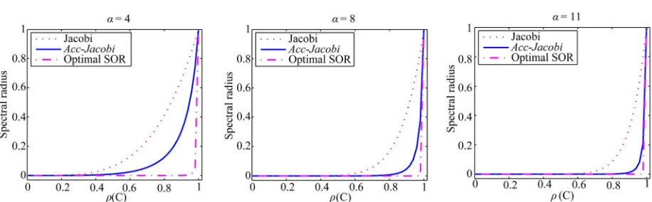
are the coefficients of the -th Che- byshev polynomial given by (20) and is define by (27). In Figure 1, we plot the curves of the Che, Jac
and SOR as functions of =
C for
0,1and = 4,8,11.
One can see clearly from these four panels that the convergence speed of the Acc-Jacobi WR iteration me- thod is sharper than that of the classical Jacobi WR iteration, while blunter than that of the optimal SOR me- thod. Moreover, as the argument becomes larger, the spectral radiuses of the Acc-Jacobi and the optimal SOR methods become nearer.
4. Numerical Results
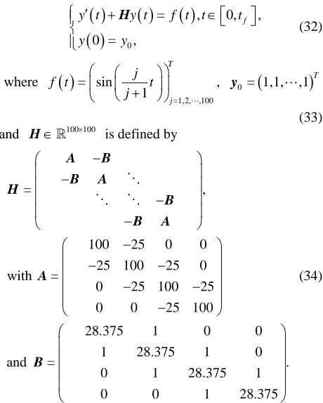
To validate our theoretical results given in Section 3, we consider the following problem:
0= , 0, ,
0 = ,
f
y t y t f t t t
y y
H
(32)
where
=1,2, ,100
= sin 1
T
j
j
f t t
j
, 0= 1,1,
,1
T
y
(33) and H100 100 is defined by
= ,
100 25 0 0
25 100 25 0
with =
0 25 100 25
0 0 25 100
28.375 1 0 0
1 28.375 1 0
and = .
0 1 28.375 1
0 0 1 28.375
A B
B A
H
B
B A
A
B
(34)
One can verify that the eigenvalue of the matrix H
defined by (34) changes from 4 10 4 to 194, and thus system (33) is really stiff. To perform the discrete-time WR iteration, we choose the backward Euler method with step size h= 0.02. Throughout all of our experiments,
we choose = 5 and N = 250, where N=tf
h is the
[image:6.595.309.539.281.568.2]
Figure 1. The spectral radius of the three discrete-time WR iterative methods; from left to right: = 4,8,11.
[image:7.595.67.527.255.387.2][image:7.595.66.527.436.503.2]
Figure 2. Measured convergence speed of the Acc-Jacobi and discrete-time Jacobi WR methods. Table 1. Coefficients
vm 5m=0 for splitting H=M1N1 and H=M2N2.coefficients vm 5m=0
splitting v0 v1 v2 v3 v4 v5
1 1
=
H M N 0 0.041 468 677 620 31 0 0.561 375 694 613 35 0 1.519 907 016 993 04
2 2
=
H M N 0 0.121 948 099 474 61 0 1.097 542 735 328 93 0 1.975 594 635 854 32
the Jacobi WR iteration. To make a fair comparison, the discrete-time Jacobi WR iteration is performed as (29). The measured error at iteration k for these two methods is defined as:
Jacobi:
1
ErrJac = max nk n
n N
k y y
, where
=1N k n
n
y and
yn Nn=1 are the k-th iterative solu- tion and the convergent solution of the discrete- time Jacobi WR method, respectively. Acc-Jacobi:
1
ErrAcc Jac = max nk n n N
k y y
, where
=1N k n
n
y and
yn nN=1 are the k-th iterative solu- tion and the convergent solution of the Acc-Jacobi method, respectively.We choose two different splitting
1 1 2 2
= =
H M N M N with M1 = diag , ,
A A,A
,
2 = diag 100,100,,100
M and N1=M1H, 2= 2
N M H. And by computer it is easy to get
1
1 1
1
2 2
1
0.543 6,
1
and 0.666 7.
h
h
I M N
I M N
For the splitting H =M1N1 and H =M2N2,
the coefficients
vm 5m=0 are given in Table 1.In Figure 2, we plot in the left and middle panels the measured error decay of the two methods with splitting
1 1
=
H M N and H =M2N2, respectively, where
one can see clearly that the convergence speed of the
and H=M2N2 with N2N1, theorem 1 predicts
that the Acc-Jacobi WR method with the former choice shall converge faster than the case with the latter one. This theoretical conclusion is clearly depicted in the right panel of Figure 2.
5. Acknowledgments
This paper is supported by the the NSF of Sichuan Uni- versity of Science and Engineering (2010XJKRL005, 2009JKRL011) and the Sichuan Provincial Education De- partment Foundation of China (10ZB098). The authors are grateful to the anonymous referees for the careful rea-ding of a preliminary version of the manscript and their valuable suggestions and comments, which really improve the quality of this paper.
6. References
[1] C. Lubich and A. Ostermann, “Multi-grid Dynamic Itera-tion for Parabolic EquaItera-tions,” BIT Numerical Mathematics, Vol. 27, No. 2, 1987, pp. 216-234.
doi:10.1007/BF01934186
[2] E. Lelarasmee, A. E. Ruehli and A. L. Sangiovanni-Vin- centelli, “The Waveform Relaxation Methods for Time- domain Analysis of Large Scale Integrated Circuits,”
IEEE Transactions on Computer-Aided Design of Inte-grated Circuits and Systems, Vol. 1, No. 3, 1982, pp. 131-145.doi:10.1109/TCAD.1982.1270004
[3] U. Miekkala and O. Nevanlinna, “Convergence of Dy-namic Iteration Methods for Initial Value Problems,”
SIAM Journal on Scientific and Statistical Computing, Vol. 8, No. 4, 1987, pp. 459-482.doi:10.1137/0908046 [4] U. Miekkala and O. Nevanlinna, “Sets of Convergence
and Stability Regions,” BIT Numerical Mathematics, Vol. 27, No.4, 1987, pp. 554-584.doi:10.1007/BF01937277 [5] U. Miekkala, “Dynamic Iteration Methods Applied to
linear DAE Systems,” Journal of Computational and Ap-plied Mathematics, Vol. 25, No. 2, 1989, pp. 133-151. doi:10.1016/0377-0427(89)90044-7
[6] O. Nevanlinna, “Remarks on Picard-Lindelöf Iteration, Part I,” BIT Numerical Mathematic, Vol. 29, No. 2, 1989, pp. 328-346.
[7] O. Nevanlinna, “Remarks on Picard-Lindelöf Iteration, Part II,” BIT Numerical Mathematic, Vol. 29, No. 3, 1989, pp. 535-562.doi:10.1007/BF02219239
[8] O. Nevanlinna, “Linear Acceleration of Picard-Lindelöf Iteration,” Numerische Mathematik, Vol. 57, No. 1, 1990, pp. 147-156.doi:10.1007/BF01386404
[9] S. Vandewalle, “Parallel Multigrid Waveform Relaxation for Parablic Problems,” B. G. Teubner, Stuttgart, 1993. [10] J. Janssen and S. Vandewalle, “Multigrid Waveform
Relaxation of Spatial Finite Element Meshes: The Conti-nuous-Time Case,” SIAM Journal on Numerical Analysis,
Vol. 33, No. 2, 1996, pp. 456-474.doi:10.1137/0733024
[11] J. Y. Pan and Z. Z. Bai, “On the Convergence of Wave-form Relaxation Methods for Linear Initial Value Prob-lems,” Journal of Computational Mathematics, Vol. 22, No. 5, 2004, pp. 681-698.
[12] J. Sand and K. Burrage, “A Jacobi Waveform Relaxation Method f or ODEs,” SIAM Journal on Scientific Com- puting, Vol. 20, No. 2, 1998, pp. 534-552.
doi:10.1137/S1064827596306562
[13] J. Wang and Z. Z. Bai, “Convergence Analysis of Two- stage Waveform Relaxation Method for the Initial Value Problems,” Journal of Applied Mathematics and Compu-ting, Vol. 172, No. 2, 2006, pp. 797-808.
doi:10.1016/j.amc.2004.11.031
[14] A. Bellen, Z. Jackiewicz and M. Zennaro, “Contractivity of Waveform Relaxation Runge-Kutta Iterations and Re-lated Limit Methods for Dissipative Systems in the Maxi-mum Norm,” SIAM Journal on Numerical Analysis, Vol. 31, No. 2, 1994, pp. 499-523.doi:10.1137/0731027 [15] L. Galeone and R. Garrappa, “Convergence Analysis of
Time-Point Relaxation Iterates for Linear Systems of Differential Equations,” Journal of Computational and Applied Mathematics, Vol. 80, No. 2, 1997, pp. 183-195. doi:10.1016/S0377-0427(97)00004-6
[16] R. Garrappa, “An Analysis of Convergence for Two-stage Waveform Relaxation Methods,” Journal of Computa-tional and Applied Mathematics, Vol. 169, No. 2, 2004, pp. 377-392.doi:10.1016/j.cam.2003.12.031
[17] J. Janssen and S. Vandewalle, “Multigrid Waveform Relaxation on Spatial Finite Element Meshes: The Dis-crete-Time Case,” SIAM Journal on Scientific Computing, Vol. 17, No. 1, 1996, pp. 133-155. doi:10.1137/0917011 [18] K. Burrage, Z. Jackiewicz and B. Welfert, “Block-Toe-
plitz Preconditioning for Static and Dynamic Linear Sys-tems,” Linear Algebra and its Applications, Vol. 279, No. 1-3, 1998, pp. 51-74.
doi:10.1016/S0024-3795(98)00007-X
[19] J. M. Bahi, K. Rhofir and J. C. Miellou, “Parallel Solu-tion of Linear DAEs by Multisplitting Waveform Relaxa-tion Methods,” Linear Algebra and its Applications, Vol. 332-334, 2001, pp. 181-196.
doi:10.1016/S0024-3795(00)00199-3
[20] C. W. Gear, “Massive Parallelism Across Space in ODEs,” Applied Numerical Mathematics, Vol. 11, No. 1-3, 1993, pp. 27-43. doi:10.1016/0168-9274(93)90038-S [21] R. S. Varga, “Matrix Iterative Analysis,” Springer Verlag,
Berlin, New York, 2000. doi:10.1007/978-3-642-05156-2 [22] Z. Z. Bai, “Parallel Matrix Multisplitting Block Relaxa-tion IteraRelaxa-tion Methods,” Mathematica Numerica Sinica, Vol. 17, No. 3, 1995, pp. 238-252.
[23] D. W. Young, “Iterative Solution of Large Linear Sys- tems,” Academic Press, New York, 1971.
[24] J. C. Mason and D. C. Handscomb, “Chebyshev Poly- nomials,” Chapman & Hall/CRC, Florida, 2003. [25] J. Janssen and S. Vandewalle, “On SOR Waveform Re-
laxation Methods,” SIAM Journal on Numerical Analysis, Vol. 34, No. 6, 1997, pp. 2456-2481.