Sensor based human activity mining using Dirichlet process mixtures of directional statistical models

Sensor-based Human Activity Mining Using

Dirichlet Process Mixtures of Directional Statistical

Models

Lei Fang

_{, Juan Ye}

_{and Simon Dobson}

St Andrews, UK

Email:⇤_{lf28@st-andrews.ac.uk,}†_{juan.ye@st-andrews.ac.uk,}‡_{simon.dobson@st-andrews.ac.uk}

Abstract—We have witnessed an increasing number of activity-aware applications being deployed in real-world environments, including smart home and mobile healthcare. The key enabler to these applications is sensor-based human activity recognition; that is, recognising and analysing human daily activities from wearable and ambient sensors. With the power of machine learning we can recognise complex correlations between various types of sensor data and the activities being observed. However the challenges still remain: (1) they often rely on a large amount of labelled training data to build the model, and (2) they cannot dynamically adapt the model with emerging or changing activity patterns over time. To directly address these challenges, we propose a Bayesian nonparametric model, i.e. Dirichlet process mixture of conditionally independent von Mises Fisher models, to enable both unsupervised and semi-supervised dynamic learning of human activities. The Bayesian nonparametric model can dynamically adapt itself to the evolving activity patterns without human intervention and the learning results can be used to alleviate the annotation effort. We evaluate our approach against real-world, third-party smart home datasets, and demonstrate significant improvements over the state-of-the-art techniques in both unsupervised and supervised settings.

I. INTRODUCTION

The European Commission has predicted that by 2025, the United Kingdom alone will see a rise of 44% in people

over 60 years of age. This motivates the development of new solutions to improve the quality of life and independence for elderly people. Ambient assisted living is one promising solution, which is enabled by sensor-based human activity recognition (HAR) – unobtrusively monitoring and inferring human activities from a collection of ambient and wearable sensors [1].

Due to its potential in healthcare, HAR has been extensively studied and numerous machine learning techniques have been applied therein. Most of them require a large number of training data well annotated with activity labels and assume a fixed model; i.e, once trained, an activity model will stay the same. However, this methodology and assumption does not reflect the complexity of real-world deployment. First of all, annotating sensor data with activity labels is known to be an intrusive, tedious, and time-consuming task. Secondly, users often change their behaviour over time; e.g., starting a new type of exercise, or changing the cooking style due to health conditions.

Unsupervised techniques such as clustering can be useful to remedy the problematic situation. They can be employed, for example, to mine clusters from the raw data for annotation, which alleviates the problem of missing labels [2]. However, most existing clustering algorithms often require some pre-knowledge from the data: for example, k-means or any other mixture model, needs to pre-fix the number of activities in advance. Moreover, once fixed, the model is hard to adapt to the evolving human behaviours over time. As a result, the practicability and performance of existing solutions are compromised. HAR system also faces other challenges includ-ing the complexity of the sensor generated data: sensor-based HAR usually employs a large number of sensors in different modalities. The high-dimensionality further complicates the learning task.

To tackle this problem we propose a Bayesian nonpara-metric directional statistical model: specifically, a Dirichlet process mixture of conditionally-independent von Mises Fisher distributions (DP-MoCIvMFs). Our solution benefits from the properties of Bayesian nonparametrics (BNP) and directional statistics on high-dimensional data, and so can dynamically discover activity patterns and automatically infer the hidden activity cluster sizes at the same time. To the best of our knowledge this is the first work that employs Dirichlet process mixture models and von Mises Fisher models together in the HAR domain, and the proposed DP-MoCIvMFs model has never been studied before in existing literature. To be specific, we claim the following novelties and contributions:

• a novel statistical model based on Dirichlet process mix-ture and conditionally independent directional statistical models for HAR activity modelling;

• a method by which activity patterns and cluster size are learnt adaptively from the data under an unsupervised setting, whereas the performance is significantly better than the state-of-the-art algorithms;

• a partially-collapsed Gibbs sampler algorithm that can make efficient on-line inference over the model and its Bayesian hierarchical extension;

with the state-of-the-art machine learning algorithms. The rest of the paper is organised as follows. Section II reviews the literature and compares and contrasts our approach with the existing work. Section III introduces the theory of von Mises-Fisher distributions and Bayesian mixture models. Section IV describes our proposed approach, which is then evaluated in Section V. We conclude our work in Section VI and point to some future work.

II. RELATED WORK

In this paper, we propose a novel generative model for unsupervised and semi-supervised learning that combines Bayesian nonparametrics and directional statistical models. In the following, we will survey the related literatures on activity recognition, BNP, directional statistical models and existing techniques in learning new types of activities and those devoted to reducing the labelling effort.

A. Activity Recognition

Activity recognition based on wearable and environmen-tal sensing technologies has been extensively researched in the last decades and a few recent surveys have broadly reviewed the existing techniques [1], [3]–[5]. In general, sensor-based activity recognition techniques can be grouped into knowledge- and driven approach, and the data-driven approach can be further classified into supervised and unsupervised learning techniques. A knowledge-driven technique leverage expert knowledge ranging from the early attempt on a small scale of common sense knowledge [6] to a more advanced and formal approach on a large scale of knowledge base such as ontologies [7] and WordNet [8], [9], and apply reasoning engines to infer activities from sensor data. A data-driven technique apply the off-the-shelf machine learning and data mining techniques to automatically establish the correlation between sensor data and activity labels. Hidden Markov Models (HMM) and recent deep neural networks are the most popular techniques [1], [10].

B. Unsupervised Learning

Unsupervised learning automatically partitions and charac-terises sensor data into patterns that can be mapped to different activities without the need of annotated training data. Pattern mining and clustering are the two mostly used techniques that support unsupervised activity recognition. Gu et al. have applied emerging patterns to mine the sequential patterns for interleaved and concurrent activities [11]. Rashidi et al. propose a method to discover the activity patterns and then manually group them into activity definitions [12]. Based on the patterns, they create a boosted version of a HMM to represent the activities and their variations in order to recognise activities in real time. Similarly, Ye et al. have combined the sequential mining and clustering algorithms to discover representative sensor events for activities. Different from the work in [12], they have applied the generic ontologies to automatically map the discovered sensor sequential patterns to activity labels through a semantic matching process [13].

Yordanova et al. have also applied domain knowledge in rule-based systems to generate probabilistic models for activity recognition [14], [15].

From statistical modelling perspective, clustering problem, or unsupervised learning can be solved by mixture models. The main focus has traditionally been on Gaussian and multinomial models. Banerjee et al. proposed an EM based inference procedure for finite mixture of von Mises Fisher (vMF) [16]. Gopal and Yang derived the Bayesian learning inferences on a finite mixture of vMFs and some other extensions like Hierarchical mixtures of vMFs [17]. Taghia et al. did similar research on Bayesian learning on vMF mixture models via variational inference [18]. The infinite mixture extension of the vMFs mixture model is first studied by Bangert et al. [19] to cluster treatment beam in external radiation therapy; while later Roge et al. propose an alternative Collapsed Gibbs sampler to infer the same infinite mixture model [20]. Qin et al. [21] developed a reverse jump Markov Chain Monte Carlo algorithm to learn trans-dimensional model of von Mises Fisher models. The major difference between our model and theirs is the component density is assumed as multiple conditional independent vMFs that accommodate both sensor and time features rather than a singular vMF.

C. Semi-supervised Learning

One of the most common semi-supervised learning tech-niques is active learning, so called “query learning”, a subfield of machine learning. It is motivated by the scenario when there is a large amount of unlabelled data but a limited and insufficient amount of labelled data. As the labelling process is tedious, time-consuming and expensive in real-world applications, active learning methods are employed to alleviate the labelling effort by selecting the most informative instances to be annotated [22].

Cheng et al. apply a density-weighted method that com-bines both uncertainty and density measure into an objective function to select the most representative instances for user annotation, which has been demonstrated to improve activity recognition accuracy with the minimal labelling effort [23]. Similarly, Hossain et al. combine the uncertainty measure and Silhouette coefficient to select the most informative instances as a way to discover new activities [24].

update procedures are based on some specific form of EM algorithm rather than a formal statistical model.

III. BACKGROUND

This section introduces the background on von Mises-Fisher distribution and its Bayesian finite mixture model, which forms the foundation of our proposed approach.

A. von Mises-Fisher Distribution

A von Mises-Fisher (vMF) distribution is a probability distribution with support on the unit hypersphere, whose density can be defined as

f(x_|µ,) =cD()eµ

T

x_{, c} D() =

D/2 1 (2⇡)D/2_I

D/2 1()

where x₂RD _{is a D dimensional vector with unit length,}

i.e. kx_k2= 1,I⌫ is the modified Bessel function of the first

kind at order ⌫, µ ₂ RD_,

kµ_k2 = 1 is the mean direction

and  > 0 is a concentration parameter indicating how

concentrated the samples are generated against µ. Whenis

large, the samples are closely aligned with µ, which tends to a point density; when is small, or close to zero, the model

degenerates to the uniform distribution on the sphere [27]. Fig. 1 shows samples from three vMFs in a three dimensional setting. Note that as  decreases, the distribution is more

uniformly spread over the sphere. vMF is a good alternative to other commonly used distributions, like Gaussian, for high dimensional data. vMF based model has been successfully applied in high dimensional data analysis, like document topic modeling [16]–[18], gene expressions [16], [18], and fMRI time series [28] etc.

-1 1 -0.5

0.5 1

0

0.5 0.5

0

0 1

-0.5

-0.5

-1 -1

Kappa = 90 Kappa = 25 Kappa = 1

Fig. 1: von Mises-Fishers with different parameters; as 

decreases, the distribution is more widespread with respect to their mean vectors µover the sphere.

B. Bayesian Mixture Model Specification

A finite mixture model assumes the data samples are inde-pendently generated by a fixed number ofK 1components.

The model implicitly assumes hidden categorical variables zi 2 {1, . . . , K}, indicating which component originally

generates xi,i= 1, . . . , N. The generative model of a finite

mixture of vMFs can be written as:

zi⇠Multi(·|⇡)

xi⇠vMF(·|µzi,zi)

where thek-th component’s vMF is defined by{µk,k}, and ⇡is the mixture proportion.

A Bayesian extension of the finite mixture model can be defined by imposing additional prior distributions on the model parameters,e.g.

⇡⇠Dirichlet(↵)

zi⇠Multi(⇡), i= 1. . . N

µk⇠vMF(m0, C0), , k= 1. . . K k⇠P0+, k= 1. . . K

xi⇠vMF(µzi,zi), i= 1. . . N

The model assumes the mixture proportion ⇡ is drawn from

a symmetric Dirichlet distribution with parameter ↵; and

each cluster’s µk and k are commonly drawn from a vMF

prior with mean and concentration parameters {m0, C0} and

some prior distribution P0+ with a strictly positive support

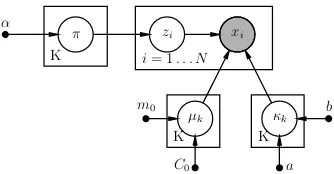
respectively. The probabilistic graphical model (PGM) rep-resentation of the Bayesian mixture of von Mises Fishers (B-movMF) is listed in Fig. 2. The Bayesian model holds various advantages over its likelihood-based counterpart, in-cluding parameter shrinkage, stability, inclusion of expert prior knowledge etc. [17]. Note that the above models require a pre-specified mixture sizeK, which is usually not feasible in real-world applications.

K _{i= 1. . . N}

K K

zi xi

µk k

a b

C0 m0

Fig. 2: The Bayesian finite mixture of vMFs in a standard probabilistic graphical model notation; whereP0+ is assumed

be identified by two parametersa, b.1

IV. PROPOSEDAPPROACH

We begin this section by describing the proposed statistical model, with the inference algorithm presented afterwards.

A. The Proposed Model

Sensor-based HAR, usually employing a large number of sensors, entails high-dimensional datasets. Inspired by the successful applications of vMFs on high-dimensional data in other domains, we propose to model sensor based activities

(after appropriate sensor feature extraction and transformation) by vMFs.

However, different classes of features are needed to differ-entiate the underlying activities, and the mixture of singular vMFs is not sufficiently flexible to capture all the character-istics. In particular, the time feature and other sensor features should ideally be treated separately as they naturally differ in many ways. Note that the time feature, upon the following cyclic transformation:

xt= (cos✓,sin✓),where✓= (h h0)⇥(2⇡/24), (1)

where h h0 is the elapsed time units between h and

any fixed reference point h0, is actually 2d vMF distributed

whereas other sensor features, after appropriate feature extrac-tion and transformaextrac-tion detailed in V-A, are of much higher dimensional directional vectors (depending on the number of deployed sensors). A more flexible approach is to treat them as multiple directional vectors on two spheres with different dimensions instead of a singular hypersphere vector.

In light of this, we propose the following conditionally independent (CI) component density. That is, conditioning on mixture identity zi (or activity identity), we assume xi

is generated by independent vMFs, i.e., decomposing xi as

the sensor features xs

i and time featurexti s.t. xi = [xsi, xti],

where xs

i andxti are unit vectors with d0 and 2 dimensions

respectively. The implied CI density of each cluster component becomes

fCI(xi|·) =vMF(xsi;µsk,sk)vMF(xti;µtk,tk). (2)

Note that at the mixture level the different data components, assumed independent atcomponentlevel, arenotindependent, due to the mixture model specification [29], implying the statistical correlations between the time and sensor features can be captured [26].

1 i= 1. . . N

1 1

1 ₁

zi xi

µs

k sk

µt

k tk

as bs at

bt

Cs ms

Ct

mt

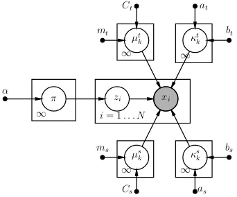
Fig. 3: The proposed DP-MCIvMF model in PGM represen-tation.

1) Dirichlet Process Mixture of CI vMFs: So far, we have assumed a finite mixture of CIvMFs (moCIvMF), where the mixture size K is constant and has to be pre-specified manually. To resolve this problem, we propose the Bayesian

non-parametric extension of the mixture model,i.e., an infinite mixture of CIvMFs, where the mixture size is assumed in-finitely large, orK_{! 1}[30]. It can be shown that the infinite mixture model induces the prior proportion⇡being generated

from a Chinese Restaurant Process (CRP), whereas the cluster component parameters are drawn from their corresponding prior distribution (or equivalently the base measure of the Dirichlet process) [30]–[32]. The CRP representation based nonparametric model can be written as:

⇡⇠CRP(↵), zi⇠Multi(⇡), i= 1. . . N

µsk ⇠vMF(ms, Cs), sk⇠G(as, bs), k= 1. . .1

µtk⇠vMF(mt, Ct), tk⇠G(at, bt), k= 1. . .1

xi⇠fCI(µtzi,

t ziµ

s zi,

s

zi), i= 1. . . N,

where the prior parameters are

{↵, ms, Cs, mt, Ct, as, bs, at, bt}. A few explanations on the

prior choices are given here. We use a Gamma distribution for  because it has the same support as the concentration

parameter (a positive real number) and it has also been shown that the likelihood function of  closely resembles a Gamma form [18]. The vMF priors for µ are used because they have the matching support and are also conjugate to vMF likelihood. The model essentially is a Dirichlet Process Mixture model with a concentration parameter ↵and a base measure induced by the prior p(µs

k, µtk,sk,tk). This model

is therefore denoted DP-MoCIvMFs hereafter. The equivalent PGM representation of the model is listed in Fig. 3. Note its differences with the Bayesian finite mixture model with singular vMF as component distribution, which is shown in Fig. 2.

B. Inference Algorithm

Based on the CRP mixture model representation, Gibbs sampling, a class of Markov Chain Monte Carlo method, can be used to make approximate Bayesian inference over the nonparametric infinite sized model [31], [32]. To improve the sampling efficiency, we employ the collapsing strategy and derive a partially collapsed Gibbs sampler [33]: the state of the chain to sample are Z = _{zi} and {sk,tk}

with the mean directions{µs

k, µtk}integrated out analytically.

Collapsing or integrating out analytically the mean direction parameters does not only saves the computation of sampling them (of high dimensional vectors, which can be expensive), but also improves the rate of convergence according to the Rao-Blackwell theorem.

As a general summary, the sampler iterate:

• Fori= 1, . . . , N, iteratively sample eachziconditioning

on the rest of the chain state, i.e. Z/i,{sk,tk} and the

observed dataX;

• Sample{sk,tk} conditioning onZ andX;

• Update prior-parameters if necessary;

p(zi =k|·)/nk, i·c2(tk)

c2(kmtCt+tk P

j2Zk /ix

t jk)

c2(kmtCt+tk P

j2Zkxt_ik)

·cd0(s_k)

cd0(kmsCs+sk P

j2Zk /ix

s jk)

cd0(kmsCs+sk P

j2Zkxs_jk)

, k= 1. . . K0 (3)

p(zi =k|·)/↵· 1

M

M X

m=1

fCI(xi|✓(m)s ,✓t(m)), k=K0+ 1

(4)

p(sk|·)/

cd0(s_k)nk

cd0(ks_kP_j2Zkxs_j+Csmsk)

G(as, bs) (5)

p(tk|·)/

c2(tk)nk

c2(ktk P

j2Zkxt_j+Ctmtk)

G(at, bt); (6)

whereK0denote the size of the occupied clusters at the current iteration; Zk _{= {j : z}

j =k} andZ_/ik ={j 6=i : zj =k};

nk =|Zk|andnk, i=|Z_/ik|, i.e. the size of the observations

in the kth cluster. And the derivation of some key results are given in the supplemental file. Some explanations over the sampling steps are given below.

Samplingzi: The sampling step forzi2{1, . . . , K0+ 1}

updates its cluster membership according to its conditional distribution. When zi = K0 + 1, i.e. eq. (4), it denotes the

probability of the observation occupying a new cluster (or new table in the CRP metaphor). Based on the CRP prior and the convoluted CIvMF base measure, the probability is proportional to

↵·

Z Z

fCI(xi|✓s,✓t)p(✓s,✓t)d✓sd✓t,

where ✓s _{= {µ}s_,s_},✓t _{= {µ}t_,t_{}. As this integral has}

no closed form solution, we resort to Monte Carlo (MC) approximation, where the MC sample size is M, and ✓_(m)s

and ✓t

(m) denote the m-th sample generated from the prior

distribution. To sample from the vMF prior, we have used the Wood method [34]. We findM = 1works well in most cases,

while a larger M leads to better converging rate in general (see the result part for some analysis on the effect of M). Note that {✓s_,✓t

} can be pre-sampled and cached for reuse in the Gibbs iterations, which greatly reduces the computation effort.

Sampling : The conditional distribution on , i.e. eq.

(5) and (6) are not of standard forms but one-dimensional distributions that can be evaluated up to some unknown constants; we therefore use slice sampler to sample them with initial starting values set as the current state [35]. Note that a slice sampler is efficient for univariate distribution sampling and it only needs to evaluate the distribution proportional to some constant.

1) On-line Inference: An important advantage of the pro-posed method is its capability to deal with on-line infer-ence: i.e. incorporation of new sensor data into the learning process as time progresses. As the time feature is explicitly

incorporated into the mixture component, the temporal order of the recorded activity data no long matters as opposed to other time series models, such as HMMs. Therefore, new data samples can be included into the sampling procedure simply as the last arriving customers of the CRP metaphor, which is in line with the exchangeability assumption of the DP mixture model [36]. Computationally speaking, as the sampler considers each data sample marginally (eq. (3) (4)), which implies new observations’ cluster membershipszis can

be sampled at the end of the hidden membership sampling step conditioning on the status of the sitting arrangements of the existing customers, and the sampling procedure can resume as normal but with expanded data size N at the following iterations.

2) Prior specification and hierarchical Bayesian model:

The prior parameters {↵, ms, Cs, mt, Ct, as, bs, at, bt} can

either be elicited from expert knowledge or learnt from data. To minimise human input, we impose a hierarchical Bayesian model to learn the prior parameters [37]. In particular, the following hyper-priors are used:

↵ 1_⇠G(1,1),

ms⇠vMF( ¯ms,0.01), mt⇠vMF( ¯mt,0.01),

bt⇠G(0.01,0.01), bs⇠G(0.01,0.01),

wherem¯s,m¯tare the maximum likelihood (ML) estimators of

the mean directions from the whole data set; while the others are fixed as constants at =as = 1 (a standard practice for

noninformative Gamma prior), Cs =Ct = 0.1

(noninforma-tive priors on the mean directions). The prior parameter update procedures can be derived based on conjugacy, which are detailed in a supplemental file that is made publicly available along with the implementation code3_.

C. (Semi-)supervised Learning

To use the DP-MoCIvMFs as a classifier, we only need to slightly modify the algorithm by treating the testing data’s labels as missing value. In an overview, a DP-MoCIvMFs can be learnt on each labelled dataset by running the Gibbs sampler in parallel; as a result, a DP-MoCIvMFs for the whole dataset can be formed; then the unlabelled data (test data) can be classified by running the Gibbs sampler to update their labels (and only their labels). The detail is listed below in Algorithm 1. The algorithm essentially creates a (flattened) hierarchical mixture of CIvMFs model for classification, where each activity is a mixture model. The novelty here is that each mixture’s size is learnt from the data rather than pre-fixed.

V. EXPERIMENT ANDEVALUATION

Algorithm 1 Semi-supervised learning of DP-MoCIvMFs

Input labelled training data_{Dc}C1 and testing dataXtest 1: foreach labelled datasetDc,c= 1. . . C do

2: Run DP-MoCIvMFs Gibbs sampler on Dc 3: Create a map from theKc clusters to classc 4: end for

5: Form a DP-MoCIvMFs on_{Dc}C1 with PC

c=1Kcclusters 6: Run the Gibbs sampler onXtest

7: MapZtestto their corresponding classes

A. Datasets and Sensor Data Pre-processing

We perform the evaluation on two real-world smart home datasets. The first dataset (House A) is collected by the Univer-sity of Amsterdam from a single-resident house instrumented with a wireless sensor network [38]. The dataset has 16 dimensions (sensors) and 7 activities. The second dataset is collected from a testbed at Washington State University2_{. This}

dataset has 32 sensors and 9 different activities.

We segment sensor events into time slots of a fixed interval. For each time slot, we extract features from the sensor data and associated timestamps. A sensor feature vector is represented as xs = [x1, x2, ..., xS], where S is the number of sensors

being installed, and each xi (1 i  S)(possibly a vector

by itself depending on the sensor type and feature extraction technique) is the extracted feature of the ith sensor. If a sensor is binary (e.g., an RFID, switch sensor, or passive infra-red motion sensor) xi is the frequency of this sensor

being activated over the interval: that is, ni/n, where ni is

the number of times the ith sensor being activated and n is the total number of sensor events reported in this time slot. For the timestamps, instead of treating them as real-valued scalar feature, we apply the transformation listed in (1).

B. Metrics and Baselines

The proposed model, DP-MoCIvMFs, is implemented in Matlab, which is made publicly available3_{. We have chosen}

a range of Bayesian/maximum likelihood based and paramet-ric/nonparametric models as baselines to give a comprehensive comparison. For non-parametric models or finite mixture mod-els, like K-means, the K is set as the true cluster size. The details of the baselines are:

• DP-MovMF: Dirichlet Process Mixture of vMFs [19], implemented in Matlab 3_;

• DP-MoG: Dirichlet Process Mixture of Gaussians, the DP base measure is the regular conjugate Normal-Inverse Wishart distribution4_;

• DP-MoCIG: Dirichlet Process Mixture of CI Gaussians, the algorithm is implemented based on the existing DP-MoG program 4_;

• K-means: the standard k-means with Euclidean distance as distance measure5_;

2_{http://ailab.wsu.edu/casas/datasets/} 3_{https://leo.host.cs.st-andrews.ac.uk} 4_{http://prml.github.io/}

5_{https://uk.mathworks.com/products/statistics.html}

• MovMF (EM): Mixture of vMFs estimated by expectation-maximization (EM) algorithm6 _[16];

• MoG (EM): Mixture of Multivariate Gaussians estimated by EM algorithm4_.

To evaluate the unsupervised learning performance, we use five standard measures for clustering algorithms [39]: mutual information (MI), normalised mutual information (NMI), Rand Index (RI), adjusted Rand Index (ARI), and Purity.

To demonstrate the classification performance of the pro-posed model, we use two criteria that are commonly used in existing literature [38] [40] to access the activity recognition accuracy, namely time-sliced wise accuracy (At) and class

wise accuracy (Ac); that is,

At=

Na

N , Ac=

1

K

K X

a=1

Aa

where Na is the number of times that an activity is

cor-rectly classified, and N is total time slice count; Aa is the

classification sensitivity rate with respect to activity a, i.e. Aa = _TPTP_a+FNa _a, where TPa and FPa denote the true

positive and false positive counts of the classifier with respect to activity a. Therefore, Ac measures the averaged by class

accuracy among all class labels. We also reportF-score to help compare the performance on both precision and sensitivity, where

F-scorea = 2⇥TPa 2_⇥TPa+FPa+FNa

.

C. Synthetic Data Analysis

We demonstrate the effectiveness of the derived sampling algorithm on two synthetically generated datasets, denotedD1

andD2. In particular, we want to examine whether the sampler

can discover the hidden clusters and infer the correct cluster size at the same time. For D1, three datasets of mixture of

K = 4 conditionally independent vMFs are generated. The dimensions of the two conditionally independent vMFs are 5 and 2 respectively. The concentration parameters of the three data sets are set as_{5,10,25_}to simulate high noise, median

noise and low noise scenarios. Each dataset has N = 100

data samples and each cluster has equal size, i.e. 25 for each cluster. The datasets for the three noise variates are collectively denoted as D1. To further challenge the algorithm and make

the generated data more similar to the real world HAR data, we generate another suite of datasets, collectively denoted as D2, with cluster sizeK= 10, dimensionD= 20, and dataset

size N = 300. Furthermore, the cluster sizes are in-balanced

among the 10 clusters to mimic the in-balanced distribution of human activities, where the size ratio between the largest and smallest cluster varies around 8. The concentration parameters are varied again among the three values to denote the high, median and low noise cases.

Table I lists the the average of 10 independent runs onD1

where K = 4 and D = 7. The initialised value of K for

TABLE I: Comparison of DP-MoCIvMF on different synthetic datasets D1 with various noise levels. The correct cluster size

is K= 4; dimensionD= 7. The paired t-test results against

DP-MoCIvMF, M=30 are denoted by a ⇤ for significance at 5% , and†for 1% level.

Dataset High Noise Med Noise Low Noise

Method/Metrics NMI K NMI K NMI K

DP-MoCIvMF M=1 .735 3.04 .849 4.08 .981 4.0

M=30 .751 3.8 .87 4.46 .983 4.0

DP-MoG .692† _{3.8 .761}† _{3.14 .636}† _2.14 DP-MoCIG .719† _{3.54 .758}† _{2.44 .786}† _2.44 K-means (K= 4) .732† _{NA .866 NA .941}† _NA

TABLE II: Comparison of DP-MoCIvMF on different syn-thetic datasetsD2with various noise levels. The correct cluster

size is K = 10; dimension D = 20; The paired t-test results against DP-MoCIvMF, M=30 are denoted by a ⇤ for significance at 5% , and †for 1% level.

Dataset High Noise Med Noise Low Noise

Method/Metrics NMI K NMI K NMI K

DP-MoCIvMF M=1 .636 8.4 0.806 8.9 .952⇤ 9.1

M=30 .657 11.1 0.807 11.1 .984 9.9

DP-MoG .509† _{5.8 .663}† _{7.3 855}† _6.3

DP-MoCIG .569† _{4.6 .669}† _{5.5 .808}† _5.4 K-means (K= 4) .641 NA .768† _{NA .911}† _NA

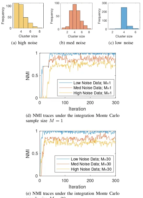
the sampler is set as 1; i.e. all the data are from one cluster. Each chain runs 200 iterations. The reportedKs are the mean of the 10 modes of the ten chains and NMIs are the average of the ten runs with the first half of each sample discarded as burn-in. Note that NMI and the inferredK value together gives a complete assessment of the clustering performance. It can be seen that the correct cluster size is recovered by the algorithm for both median and low noise cases while the algorithm’s performance on high noise data deteriorates slightly. The Monte Carlo sample size M does not affect the performance much, as the deviance is not significant. The results of some other models/algorithms on the same datasets are also listed for reference.

To better understand the distribution or uncertainty of K and the effect of the Monte Carlo sample sizeM, results from some individual runs are plotted in Fig 4. The histograms of the inferred cluster size with the sampler with M = 1 are

shown in the top row (the results withM = 30is very similar).

It is evident that the uncertainty grows as the data becomes noisier. But the correct size 4 is always within the highest

credible interval, which shows the proposed algorithm can successfully infer the cluster size from the data. The lower two figures show the NMI traces of two samplers withM = 1and

30 respectively. In general, the sampler withM = 1converges

slower (stuck at some local maximum initially) but eventually mix well, and there is no significant difference between the converged results of the two settings.

Table II lists the results onD2whereK= 10andD= 20.

The overall results show a very similar pattern as the D1’s,

although the Monte Carlo sample size M seems affect the performance a bit more for this more complicated dataset, as the deviance is slightly greater. Also the correct cluster size can be inferred from the data by the algorithm for the low-noise case while the algorithm’s performance on median-low-noise data is slightly off the target although the difference is minor (within 1 on average).

(a) high noise (b) med noise (c) low noise

0 100 200 300

Iteration

0 0.5 1

NMI

Low Noise Data; M=1 Med Noise Data; M=1 High Noise Data; M=1

(d) NMI traces under the integration Monte Carlo sample sizeM= 1

0 100 200 300 Iteration

0 0.5 1

NMI _{Low Noise Data; M=30}

Med Noise Data; M=30 High Noise Data; M=30

(e) NMI traces under the integration Monte Carlo sample sizeM= 30

Fig. 4: Evaluations on synthetic data set D1; the top three

figures show the inferred cluster size under the three data sets, and the Monte Carlo sample size M = 1is used; the lower

two figures show the NMI against the running iterations on bothM = 1 (left) andM = 30(right) settings.

D. Unsupervised Learning on Real World Sensor Data

TABLE III: Experiment results on House A data. The paired t-test results are denoted by⇤ for significance at 5% , and†for 1% level.

Method/Metric NMI MI Rand Index Adjusted RI Purity

DP-MoCIvMFs .690 (.032) 2.159 (.118) .875 (.008) .493 (.039) .892 (.034) DP-MoCIvMFs on-line .690 (.011) 2.185 (.0437) .872 (.004) .471 (.025) .901 (.015)

DP-MovMF .619 (.047)† _{2.089 (.252)}† _{.835 (.016)}† _{.280 (.041)}† _{.857 (.076)}⇤ DP-MoG .530 (.060)† _{1.144 (.151)}† _{.739 (.058)}† _{.3783 (.092)}† _{.580 (.037)}† DP-MoCIG .566 (.049)† _{1.315 (.146)}† _{.804 (.042)}† _{.475 (.081) .616 (.035)}† K-means .519 (.039)† _{1.354 (.114)}† _{.791 (.018)}† _{.304 (.045)}† _.619(.053)† MovMF .474 (.045)† _{1.190 (.127)}† _{.756 (.022)}† _{.251 (.046)}† _{.592 (.041)}† MoG .489 (.062)† _{1.061 (.192)}† _{.713 (.086)}† _{.344 (.117)}† _{.536 (.082)}†

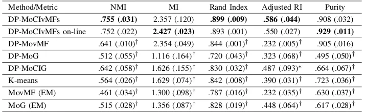
TABLE IV: Experiment results on Washington data. The paired t-test results are denoted by ⇤ for significance at 5% , and† for 1% level.

Method/Metric NMI MI Rand Index Adjusted RI Purity

DP-MoCIvMFs .755 (.031) 2.357 (.120) .899 (.009) .586 (.044) .908 (.032) DP-MoCIvMFs on-line .752 (.022) 2.427 (.023) .893 (.001) .550 (.027) .929 (.011)

DP-MovMF .641 (.010)† _{2.354 (.049) .844 (.001)}† _{.232 (.005)}† _{.905 (.016)} DP-MoG .512 (.055)† _{1.116 (.164)}† _{.720 (.043)}† _{.323 (.068)}† _{.495 (.050)}† DP-MoCIG .642 (.058)† _{1.626 (.155)}† _{.830 (.032)}† _{.487 (.093)}⇤ _{.664 (.067)}† K-means .564 (.026)† _{1.629 (.074)}† _{.842 (.008)}† _{.390 (.031)}† _{.723 (.036)}† MovMF (EM) .461 (.034)† _{1.300 (.098)}† _{.787 (.016)}† _{.232 (.035)}† _{.630 (.037)}† MoG (EM) .515 (.028)† _{1.356 (.087)}† _{.828 (.019)}† _{.448 (.064)}† _{.617 (.028)}†

evaluation metric. Statistical significance tests results against DP-MoCIvMF are denoted by a⇤for significance at 5% level and†for 1%. The reported values are the means and standard deviations of the ten runs with the the first half of the chains discarded as burn in.

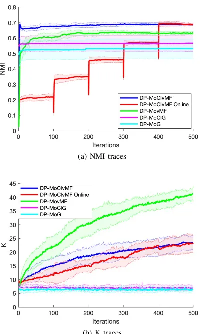
To assess the algorithm’s performance on on-line inference, we also simulate the scenario by segmenting the whole dataset randomly into equal subsets and feed the algorithm incremen-tally at some sampling frequency (every 100 iterations). In reality, it is similar to adding operational observations at some fixed frequency e.g.every 60 mins.

Based on the results, it is evident that the proposed model, either on-line or off-line, perform the best among the listed clustering methods across the five metrics. It is interesting to note that the vMF based methods outperform their Gaussian equivalences, which supports our claim vMFs are suitable for sensor based human activity modelling. The difference between the Gaussian models and CIvMF models is greater in Washington dataset where the data dimension is larger and Gaussian models struggles to fit (whose parameter size grows in(O(D2_{))comparing toO(D)for vMF). Comparing}

with other vMF based methods, DP-MoCIvMFs also achieves better results, which demonstrates the effectiveness of the DP-mixture and CI assumption. The purity measures how pure each formed cluster with respect to the true label. The good performance of DP-MoCIvMFs on this metric indicates the algorithm’s potential in alleviating data annotation effort. The on-line inference of DP-MoCIvMFs achieves comparable results as its off-line counterpart, where the differences are insignificant; this shows the proposed solution’s capability in

handling the on-line learning scenario, a desirable property for long term deployed HAR systems.

(a) NMI traces

(b) K traces

Fig. 5: NMI traces and inferred K values against iteration on House A Dataset; the bold colored lines are the mean values at each iteration while the shaded area are +/ standard deviation against the iteration means.

E. Semi-supervised Learning

In this section, we evaluate how the proposed solution works as an activity classifier under the supervised learning setting (as detailed in IV-C). We evaluate the method again on the two real world datasets. The results are reported in Table V and VI respectively. We compare the proposed solution against a wide range of generative and discriminative classification algorithms. In particular, we compare it with three other statistical model based classifiers, namely Mixture of Gaus-sians (MoG) and Mixture of von Mises Fisher (MovMFs) both of which are estimated by maximum likelihood method, while DP-MovMF and DP-MoCIvMFs are learnt based on the proposed Gibbs sampler based algorithm. In addition, we also list the results of a few widely used discriminative classifiers: Neural Networks (NNet), Support Vector Machine (SVM), K-Nearest Neighbour (KNN), and Random Forest. All the listed discriminative classifiers are implemented in Matlab’s Statistic and Machine Learning toolbox. A five-fold cross validation is used for this comparison.

According to the results, the overall stronger performance

of the discriminative classifiers over generative ones echos existing research findings [41]. Nevertheless, it is evident that the DP-MoCIvMFs is a strong candidate for activity classifica-tion. Its performance is the best among all generative models and comparable or better than most of the discriminative classifiers.

TABLE V: Comparing classification accuracy on House A data.

Method By Time Slice By Class F-score NNet .912 (.031) .874 (.051) .874 (.043) SVM .92 (.019) .847 (.013) .851 (.02) KNN .912 (.03) .88 (.051) .884 (.054) Random Forest .926 (.03) .899 (.06) .895 (.036) MoG .887 (.044) .875 (.058) .857 (.048) MovMF .796 (.024) .823 (.04) .793 (.031) DP-MovMF .895 (.022) .853 (.047) .85 (.059) DP-MoCIvMFs .932 (.03) .901 (.052) .91 (.054)

TABLE VI: Comparing classification accuracy on Washington data.

Method By Time Slice By Class F-score NNet .905 (.023) .8 (.051) .787 (.038) SVM .927 (.011) .803 (.022) .801 (.014) KNN .922 (.021) .814 (.061) .819 (.059) Random Forest .926 (.015) .822 (.035) .815 (.029) MoG .65 (.05) .678 (.065) .618 (.073) MovMF .754 (.036) .739 (.049) .675 (.039) DP-MovMF .884 (.028) .812 (.053) .783 (.039)) DP-MoCIvMFs .939 (.019) .852 (.059) .836 (.048)

VI. CONCLUSION AND FUTURE WORK

This paper proposes a novel generative statistical model for human activity mining. It supports unsupervised and semi-supervised learning for human activity recognition, without the need for any pre-knowledge on the number or the profiles of potential activities. It can not only reduce the burden of labelling sensor data, but also support inference over dynam-ically evolving activities. We have evaluated the proposed approach on synthesised and real-world smart home datasets and compared with a wide range of alternative approaches. The evaluation results have demonstrated the proposed solu-tion’s capabilities in both unsupervisedly clustering HAR data without fixing the cluster size and supervisedly learning the label correctly.

ACKNOWLEDGEMENT

This work has been partially supported by the UK EPSRC under grant number EP/N007565/1, “Science of Sensor Sys-tems Software”.

REFERENCES

[1] J. Ye, S. Dobson, and S. McKeever, “Situation identification techniques in pervasive computing: a review,” Pervasive and mobile computing, vol. 8, pp. 36–66, Feb. 2012.

[2] J. Ye, G. Stevenson, and S. Dobson, “Usmart,” ACM Transactions on Interactive Intelligent Systems, vol. 4, no. 4, pp. 1–27, Nov 2014. [Online]. Available: http://dx.doi.org/10.1145/2662870

[3] J. Aggarwal and M. Ryoo, “Human activity analysis: A review,”ACM Comput. Surv., vol. 43, no. 3, pp. 16:1–16:43, Apr. 2011. [Online]. Available: http://doi.acm.org/10.1145/1922649.1922653

[4] L. Chen, J. Hoey, C. Nugent, D. Cook, and Z. Yu, “Sensor-based activity recognition,”IEEE Transactions on Systems, Man, and Cybernetics, Part C, vol. 42, no. 6, pp. 790–808, 2012.

[5] O. D. Lara and M. A. Labrador, “A survey on human activity recogni-tion using wearable sensors,”IEEE Communications Surveys Tutorials, vol. 15, no. 3, pp. 1192–1209, Third 2013.

[6] S. W. Loke, “Representing and reasoning with situations for context-aware pervasive computing: a logic programming perspective,” The Knowledge Engineering Review, vol. 19, no. 03, pp. 213–233, 2004. [7] J. Ye, S. Dasiopoulou, G. Stevenson, G. Meditskos, E. Kontopoulos,

I. Kompatsiaris, and S. Dobson, “Semantic web technologies in pervasive computing: A survey and research roadmap,”Pervasive and Mobile Computing, vol. 23, pp. 1 – 25, 2015. [Online]. Available: http://www.sciencedirect.com/science/article/pii/S1574119214001989 [8] W. Kleiminger, F. Mattern, and S. Santini, “Predicting household

occupancy for smart heating control: A comparative performance analysis of state-of-the-art approaches,”Energy and Buildings, vol. 85, pp. 493 – 505, 2014. [Online]. Available: http://www.sciencedirect. com/science/article/pii/S037877881400783X

[9] E. Tapia, T. Choudhury, and M. Philipose, “Building reliable activity models using hierarchical shrinkage and mined ontology,” inPervasive ’06. Springer Berlin Heidelberg, 2006, pp. 17–32.

[10] J. Wang, Y. Chen, S. Hao, X. Peng, and L. Hu, “Deep learning for sensor-based activity recognition: A survey,” Pattern Recognition Letters, 2018. [Online]. Available: http://www.sciencedirect.com/science/article/ pii/S016786551830045X

[11] T. Gu, Z. Wu, X. Tao, H. K. Pung, and J. Lu, “epsicar: An emerging patterns based approach to sequential, interleaved and concurrent activity recognition,” in 2009 IEEE International Conference on Pervasive Computing and Communications, March 2009, pp. 1–9.

[12] P. Rashidi, D. J. Cook, L. B. Holder, and M. Schmitter-Edgecombe, “Discovering activities to recognize and track in a smart environment,” IEEE Trans. on Knowl. and Data Eng., vol. 23, no. 4, pp. 527–539, Apr. 2011.

[13] J. Ye, G. Stevenson, and S. Dobson, “Usmart: An unsupervised semantic mining activity recognition technique,”ACM Trans. Interact. Intell. Syst., vol. 4, no. 4, pp. 16:1–16:27, Nov. 2014. [Online]. Available: http://doi.acm.org/10.1145/2662870

[14] K. Yordanova and T. Kirste, “A process for systematic development of symbolic models for activity recognition,”ACM Trans. Interact. Intell. Syst., vol. 5, no. 4, pp. 20:1–20:35, Dec. 2015. [Online]. Available: http://doi.acm.org/10.1145/2806893

[15] F. Kruger, M. Nyolt, K. Yordanova, A. Hein, and T. Kirste, “Computational state space models for activity and intention recognition. a feasibility study,”PLOS ONE, vol. 9, pp. 1–24, 11 2014. [Online]. Available: https://doi.org/10.1371/journal.pone.0109381

[16] A. Banerjee, I. S. Dhillon, J. Ghosh, and S. Sra, “Clustering on the unit hypersphere using von mises-fisher distributions,” J. Mach. Learn. Res., vol. 6, pp. 1345–1382, Dec. 2005. [Online]. Available: http://dl.acm.org/citation.cfm?id=1046920.1088718

[17] S. Gopal and Y. Yang, “Von mises-fisher clustering models,” in Inter-national Conference on Machine Learning, 2014, pp. 154–162. [18] J. Taghia, Z. Ma, and A. Leijon, “Bayesian estimation of the von-mises

fisher mixture model with variational inference,”IEEE Transactions on Pattern Analysis and Machine Intelligence, vol. 36, no. 9, pp. 1701– 1715, Sept 2014.

[19] M. Bangert, P. Hennig, and U. Oelfke, “Using an infinite von mises-fisher mixture model to cluster treatment beam directions in external radiation therapy,” in Machine Learning and Applications (ICMLA), 2010 Ninth International Conference on. IEEE, 2010, pp. 746–751. [20] E. Rogers, J. D. Kelleher, and R. J. Ross, “Using topic modelling

algorithms for hierarchical activity discovery,” inAmbient Intelligence-Software and Applications–7th International Symposium on Ambient Intelligence (ISAmI 2016). Springer, 2016, pp. 41–48.

[21] X. Qin, P. Cunningham, and M. Salter-Townshend, “Online trans-dimensional von mises-fisher mixture models for user profiles,”Journal of Machine Learning Research, vol. 17, no. 200, pp. 1–51, 2016. [Online]. Available: http://jmlr.org/papers/v17/15-454.html

[22] B. Settles, “Active learning literature survey,” University of Wisconsin– Madison, Computer Sciences Technical Report 1648, 2009.

[23] H.-T. Cheng, F.-T. Sun, M. Griss, P. Davis, J. Li, and D. You, “Nu-activ: Recognizing unseen new activities using semantic attribute-based learning,” inProceeding of the 11th annual international conference on Mobile systems, applications, and services. ACM, 2013, pp. 361–374. [24] H. S. Hossain, N. Roy, and M. A. A. H. Khan, “Active learning enabled activity recognition,” in 2016 IEEE International Conference on Pervasive Computing and Communications (PerCom). IEEE, 2016, pp. 1–9.

[25] H. Alemdar, T. L. van Kasteren, and C. Ersoy, “Using active learning to allow activity recognition on a large scale,” in International Joint Conference on Ambient Intelligence. Springer, 2011, pp. 105–114. [26] L. Fang, J. Ye, and S. Dobson, “Discovery and recognition of emerging

human activities using a hierarchical mixture of directional statistical models,”IEEE Transactions on Knowledge and Data Engineering, pp. 1–1, 2019.

[27] K. V. Mardia and P. E. Jupp,Directional Statistics. Wiley, 2008. [28] R. E. Røge, K. H. Madsen, M. N. Schmidt, and M. Mørup, “Infinite

von mises-fisher mixture modeling of whole brain fmri data,” Neural Comput., vol. 29, no. 10, pp. 2712–2741, Oct. 2017. [Online]. Available: https://doi.org/10.1162/neco a 01000

[29] C. M. Bishop,Pattern Recognition and Machine Learning (Information Science and Statistics). Berlin, Heidelberg: Springer-Verlag, 2006. [30] C. E. Rasmussen, “The infinite gaussian mixture model,” inIn Advances

in Neural Information Processing Systems 12. MIT Press, 2000, pp. 554–560.

[31] M. D. Escobar and M. West, “Bayesian density estimation and inference using mixtures,” Journal of the American Statistical Association, vol. 90, no. 430, pp. 577–588, 1995. [Online]. Available: https://www.tandfonline.com/doi/abs/10.1080/01621459.1995.10476550 [32] R. M. Neal, “Markov chain sampling methods for dirichlet process mixture models,” Journal of Computational and Graphical Statistics, vol. 9, no. 2, pp. 249–265, 2000. [Online]. Available: http: //www.jstor.org/stable/1390653

[33] J. S. Liu, “The collapsed gibbs sampler in bayesian computations with applications to a gene regulation problem,” Journal of the American Statistical Association, vol. 89, no. 427, pp. 958–966, 1994.

[34] A. T. Wood, “Simulation of the von mises fisher distribution,” Commu-nications in statistics-simulation and computation, vol. 23, no. 1, pp. 157–164, 1994.

[35] R. M. Neal, “Slice sampling,”Ann. Statist., vol. 31, no. 3, pp. 705–767, 06 2003. [Online]. Available: https://doi.org/10.1214/aos/1056562461 [36] D. J. Aldous, “Exchangeability and related topics,” in ´Ecole d’´et´e de

probabilit´es de Saint-Flour, XIII—1983, ser. Lecture Notes in Math. Berlin: Springer, 1985, vol. 1117, pp. 1–198. [Online]. Available: http://www.springerlink.com/content/c31v17440871210x/fulltext.pdf [37] A. Gelman, J. B. Carlin, H. S. Stern, and D. B. Rubin,Bayesian Data

Analysis, 2nd ed. Chapman and Hall/CRC, 2004.

[38] T. van Kasteren, A. Noulas, G. Englebienne, and B. Kr¨ose, “Accurate activity recognition in a home setting,” inUbiComp ’08: Proceedings of the 10th International Conference on Ubiquitous Computing. Seoul, Korea: ACM, Sep. 2008, pp. 1–9.

[39] D. M. Christopher, R. Prabhakar, and S. Hinrich, “Introduction to information retrieval,” An Introduction To Information Retrieval, vol. 151, no. 177, p. 5, 2008.

[40] N. C. Krishnan and D. J. Cook, “Activity recognition on streaming sen-sor data,”Pervasive and Mobile Computing, 2012. [Online]. Available: http://www.sciencedirect.com/science/article/pii/S1574119212000776 [41] A. Y. Ng and M. I. Jordan, “On discriminative vs. generative classifiers: