Foundations of the AdS 5 x S^5 Superstring Part I

(1)

arXiv:0901.4937v2 [hep-th] 28 May 2009

ITP-UU-09-05 SPIN-09-05 TCD-MATH-09-06 HMI-09-03

Foundations of the

AdS

5

×

S

5

Superstring

Part I

Gleb Arutyunova∗† _{and Sergey Frolov}b∗†

a _{Institute for Theoretical Physics and Spinoza Institute,}

Utrecht University, 3508 TD Utrecht, The Netherlands

b _{Hamilton Mathematics Institute and School of Mathematics,}

Trinity College, Dublin 2, Ireland

Abstract

We review the recent advances towards finding the spectrum of the AdS5 ×S5

superstring. We thoroughly explain the theoretical techniques which should be useful for the ultimate solution of the spectral problem. In certain cases our exposition is original and cannot be found in the existing literature. The present Part I deals with foundations of classical string theory in AdS5×S5, light-cone perturbative

quantiza-tion and derivaquantiza-tion of the exact light-cone world-sheet scattering matrix.

∗_{Email: [email protected], [email protected]}

(2)

Introduction

Already in the mid seventies it became clear that the existing theoretical tools are hardly capable of providing an ultimate solution to the theory of strong interactions – Quantum Chromodynamics (QCD). At small distances quarks interact weakly and the physical properties of the theory can be well described by perturbative expan-sion based on Feynman diagrammatics. However, at large separation, forces between quarks become strong and this precludes the usage of perturbation theory. Under-standing the strong coupling dynamics of quantum Yang-Mills theories remains one of the daunting challenges of theoretical particle physics.

A spectacular new insight into dynamics of non-abelian gauge fields has recently been offered by the AdS/CFT (Anti-de-Sitter/Conformal Field Theory) duality con-jecture also known under the name of the “gauge-string correspondence” [1]. This conjecture states that certain four-dimensional quantum gauge theories could be al-ternatively described in terms of closed strings moving in a ten-dimensional curved space-time.

The prime example of the gauge-string correspondence involves the four-dimen-sional maximally-supersymmetric_N = 4 Yang-Mills theory with gauge group SU(N) and type IIB superstring theory defined in an AdS5 ×S5 space-time, which is the

product of a five-dimensional Anti-de-Sitter space (the maximally symmetric space of constant negative curvature) and a five-sphere. Since no candidate for a string dual of QCD is presently known, the _N = 4 theory together with its conjectured string partner offers a unique playground for testing the correspondence between strings and quantum field theories, as well as for understanding strongly-coupled gauge theories in general. The success of the whole gauge-string duality program relies on our ability to quantitatively verify this prime example of the correspondence and, more importantly, to clarify the physical principles at work.

(6)

share the same kinematical symmetry. This, however, does not a priory imply their undoubted equivalence.

To solve a conformal field theory, one has to identify the spectrum of primary op-erators (forming irreducible representations of the conformal group) and to compute their three-point correlation functions. Scaling (conformal) dimensions of primary operators and the three-point correlators encode all the information about the theory since all higher-point correlation functions can in principle be found by using the Operator Product Expansion. The _N = 4 theory has two parameters: the coupling constantgYM and the rankN of the gauge group, and it admits a well-defined ’t Hooft

expansion in powers of 1/N with the ’t Hooft coupling λ = g2

YMN kept fixed. The

AdS/CFT duality conjecture relates these parameters to the string coupling constant

gs and the string tension g as follows: gs = λ/4πN and g = √

λ/2π. Scaling di-mensions ∆ of composite gauge invariant primary operators are eigenvalues of the dilatation operator and they depend on the couplings: ∆ _≡ ∆(λ,1/N). Scaling di-mension is the only label of a (super)-conformal representation which is allowed to continuously depend on the parameters of the model. In spite of the finiteness of the _N = 4 theory, composite operators undergo non-trivial renormalization which explains the appearance of coupling-dependent anomalous dimensions. Alternatively, in string theory on AdS5×S5 energiesE of string states are functions of the couplings:

E _≡E(g, gs). In the most general setting, the gauge-string duality conjecture implies

that physical states of gauge and string theories are organized in precisely the same set of psu(2,2|4)-multiplets. In particular, energies of string states measured in the global AdS coordinates must coincide with scaling dimensions of gauge theory pri-mary operators, both regarded as non-trivial functions of their couplings. Exhibiting this fact would be the first important step towards proving the conjecture.

The initial research on theN = 4 gauge-string duality was concentrated on deriv-ing scalderiv-ing dimensions/correlation functions of primary operators in the supergravity approximation [2, 3]. This corresponds to the strongly-coupled planar regime in the gauge theory where λ is infinite and N is large. Only rather special states – those which are protected from renormalization by a large amount of supersymmetry – could be a subject of comparison here.

The next important step has been undertaken in [4], where a special scaling limit was introduced. This work initiated intensive studies of unprotected operators with large R-charge which eventually led to the discovery of integrable structures in the gauge theory [5]-[7]. This discovery marked a new phase in the research on the fundamental model of AdS/CFT.

In the limit where the rank of the gauge group becomes infinite, one can neglect string interactions and consider free string theory. Free strings propagating in a non-trivial gravitational background such as AdS5×S5 are described by a two-dimensional

(7)

Non-linear Sigma Model

in 2D

Quantum Field Theory

in 4D

Figure 1: The AdS/CFT correspondence: The spectrum of a 2d non-linear sigma-model describing string theory on a curved background is expected to be equivalent to the spectrum of a 4d quantum non-abelian gauge theory in the largeN limit.

In general, to solve a non-linear quantum sigma model would be a hopeless en-terprise. Remarkably, it appears, however, that classical strings in AdS5 ×S5 are

described by an integrable model [8]. Integrable models constitute a special class of dynamical systems with an infinite number of conservation laws which in many cases hold the key to their exact solution. If string integrability continues to exist for the corresponding quantum theory then we are facing a breathtaking possibility to solve the string model exactly and, via the gauge-string duality, to find an exact solution of an interacting quantum field theory in four dimensions.

In recent years there has been a lot of exciting progress towards understanding integrable properties of both the string sigma model and the dual gauge theory. Not all this progress is yet logically deducible from the first principles and in certain cases it is based on new assumptions or clever guesses. Nevertheless, we feel that a clear and self-contained picture starts to emerge of how to obtain a solution (spectrum) of quantum strings in AdS5×S5. It is the scope of this review to explain this picture

and to provide all the necessary technical tools in its support.

The review should be accessible to PhD students. It is certainly desirable to have a prerequisite knowledge of string theory [9]. The review might also be useful for specialists: as a handbook and as a source of formulae. In order not to distract the reader’s attention with references, we comment on the literature in a special section concluding each chapter. Further, we emphasize that this review is most exclusively about string theory. To get more familiar with gauge theory constructions, the reader is invited to consult the original literature and reviews [10, 11].

(8)

Light-cone gauge

The starting point is the Green-Schwarz action for strings in AdS5×S5 which defines

a two-dimensional non-linear sigma model of Wess-Zumino type [12]. The isometries of the AdS5 ×S5 space-time constitute the global symmetry algebra of the sigma

model and string states are naturally characterized by the charges (representation labels) they carry under this symmetry algebra. Among all representation labels two charges, J and E, are of particular importance for the light-cone gauge fixing. The charge J is the angular momentum carried by the string due to its rotation around the equator of S5 _and _E _{is the string energy, the latter corresponds to the symmetry}

of the Green-Schwarz action under constant shifts of the global time coordinate of the AdS space. It is the energy spectrum of string states that we would like to determine and subsequently compare to the spectrum of scaling dimensions of primary operators in the gauge theory.

To describe the physical states, it is advantageous to fix the so-called generalized light-cone gauge. In this gauge the world-sheet Hamiltonian is equal to E−J, while the light-cone momentum P+ is another global charge which, generically, is a linear

combination ofJ and E. Physical states should satisfy the level-matching condition: the total world-sheet momentum carried by a state must vanish. Solving the model is then equivalent to computing the physical spectrum of the (quantized) light-cone Hamiltonian for a fixed value of P+.

Fixing the light-cone gauge for the Green-Schwarz string in a curved background is subtle because of a local fermionic symmetry. This question has been studied in [13, 14] where the exact gauge-fixed classical Hamiltonian was found. This Hamiltonian is non-polynomial in the world-sheet fields and, as such, can hardly be quantized in a straightforward manner.

From cylinder to plane: Decompactification and symmetries

In the light-cone gauge the world-sheet action depends explicitly on the light-cone momentum P+. By appropriately rescaling the world-sheet coordinates, the theory

becomes defined on a cylinder of circumference P+. At this stage, one can consider

the decompactification limit, i.e. the limit where P+ and therefore the radius of the

cylinder go to infinity, while keeping the string tension fixed. In this limit one is left with a theory on a plane which leads to significant simplifications. Most importantly, the world-sheet theory has a massive spectrum and the notion of asymptotic states (particles) is well defined, calling for an application of scattering theory. Quantum integrability should then imply the absence of particle production and factorization of multi-particle scattering into a sequence of two-body events.

(9)

sym-metry algebra of the model. Namely, the manifest psu(2_|2)_⊕psu(2_|2)_⊂ psu(2,2_|4) symmetry algebra of the light-cone string theory gets enhanced by two central charges [15]. The central charges vanish on physical states satisfying the level-matching con-dition but they play a crucial role in fixing the structure of the world-sheet S-matrix. The same centrally-extended algebra also appears in the dual gauge theory [16].

Dispersion relation and scattering matrix

Insights coming from both gauge and string theory [4] led to a conjecture for the dispersion relation [17]. It has the following unusual form

ǫ(p) =

r

1 + 4g2_sin2 p

2,

where g is the string tension, ǫ and p are the energy and the momentum of an elementary excitation.

An important observation made in [16] is that the dispersion relation is uniquely determined by the symmetry algebra of the model provided its central charges are known as exact functions of the string tension and the world-sheet momentum. The dispersion relation is non-relativistic although it reveals the usual square root de-pendence of relativistic field theory. On the other hand, the sine function under the square root is a common feature of lattice theories, and its appearance here is rather surprising, given that the string world-sheet is continuous.

The various pieces of the two-body scattering matrix were conjectured in [18, 19, 21] based on the analysis of the integral equations [22] describing classical spinning strings [23, 24, 25] and insights from gauge theory [17]. Later, it was found that the matrix structure of this S-matrix is uniquely fixed by the centrally-extended

psu(2_|2)_⊕psu(2_|2) symmetry algebra, the Yang-Baxter equation and the generalized physical unitarity condition [16, 26, 27].

Dressing factor

The S-matrix is thus determined up to an overall scalar function σ(p1, p2) – the

so-called dressing factor [18]. Ideally, one would hope that further physical requirements would allow for complete determination of this factor. In relativistic integrable quan-tum field theories implementation of Lorentz invariance together with crossing sym-metry exchanging particles with anti-particles imposes an additional crossing relation on the S-matrix [28].

(10)

Luckily, the logarithm of the dressing factor turns out to be a two-form on the vector space of local conserved charges of the model which severely constraints its functional form [18]. The dressing factor explicitly depends on the string tension g

and admits a “strong coupling” expansion in powers of 1/g that corresponds to an asymptotic perturbative expansion of the string sigma model.

Combining the functional form of the dressing factor together with the first two known orders in the strong coupling expansion [18, 30], a set of solutions to the crossing equation in terms of an all-order strong coupling asymptotic series has been proposed [31]. A particular solution was conjectured to correspond to the actual string sigma model perturbative expansion. This solution was shown to agree with the explicit two-loop sigma model result [32, 33]. It should be stressed, however, that all these solutions are only asymptotic and, therefore, they do not define the dressing factor as a function of g.

In contrast to the strong coupling expansion, gauge theory perturbative expansion of the dressing factor is in powers of g and it has a finite radius of convergence. As a result, the dressing factor can be defined as a function of g. An interesting proposal for the exact dressing factor has been put forward in [34]. On the one hand, it agrees with the explicit four-loop gauge theory computation [35, 36]. On the other hand, it was argued to have the same strong coupling asymptotic expansion as the particular solution by [31] corresponding to the string sigma model. Taking all this into account, one can adopt the working assumption that the exact dressing factor and, therefore, the S-matrix are established. However, a word of caution to bear in mind – there is no unique solution to the crossing equation; additional yet to be found physical constraints should be used to single out the right solution unambiguously.

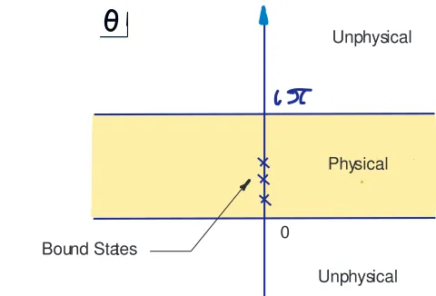
Bound states

Having found the exact dispersion relation and the S-matrix, the next step is to determine the complete asymptotic spectrum of the model. This amounts to finding all bound states of the elementary excitations and bound states of the bound states, etc. This problem can be solved by analyzing the pole structure of the S-matrix. The analysis reveals that all bound states are those of elementary particles [37]. More explicitly, Q-particle bound states comprise into the tensor product of two 4Q-dim atypical totally symmetric multiplets of the centrally-extended symmetry algebra

su(2|2) [38]. Since the light-cone string sigma model is not Lorentz-invariant, the identification of what is called the “physical region” of the S-matrix is very subtle and it affects the counting of bound states [27].

(11)

Back from plane to cylinder: Finite P+ spectrum

Having understood the spectrum of the light-cone string sigma model on a plane, one has to “upgrade” the findings to a cylinder. All physical string configurations (and dual gauge theory operators) are characterized by a finite value of P+, and as such

they are excitations of a theory on a cylinder.

The first step in determining the finite-size spectrum of a two-dimensional inte-grable model is to consider the model on a cylinder of a very large but finite cir-cumference P+. In this case integrability implies that a multi-particle state can be

approximately described by the wave function of the Bethe-type [28]. Factorizability of the multi-particle scattering matrix together with the periodicity condition for the Bethe wave function leads to a system of equations on the particle momenta known as the Bethe-Yang equations. In the AdS/CFT context these equations are usually referred to as the asymptotic Bethe ansatz1 _{[21]. The AdS}

5 ×S5 string S-matrix

has a complicated matrix structure which results at the end in a set of nested Bethe equations [21, 16, 42].

The Bethe-Yang equations determine any power-like 1/P+ corrections to the

en-ergy of multi-particle states. It is known, however, that for large P+ there are also

exponentially small corrections. To compute the leading exponential corrections, one can adapt L¨uscher’s formulae [43, 44] for the non-Lorentz-invariant case at hand [45]. This computation has been done for some string states at strong coupling.

Remarkably, L¨uscher’s approach could be also applied to find perturbative scaling dimensions of gauge theory operators up to the first order where the Bethe-Yang description breaks down [46]. The corresponding computation has been done [46] for the simplest case of the so-called Konishi operator and stunning agreement with a very complicated four-loop result based on the standard Feynman diagrammatics [47] has been found. String theory starts to reveal its extreme power, elegance and simplicity in comparison to the conventional perturbative approach!

Thermodynamic Bethe Ansatz

The success in computing gauge theory perturbative anomalous dimensions is very encouraging. However, one is really interested in non-perturbative gauge theory, i.e.

in the exact spectrum for finite values of the gauge coupling (or equivalently for finite string tension and finite P+). One tempting possibility is to generalize the

thermodynamic Bethe ansatz (TBA), originally developed for relativistic integrable models [48], to the light-cone string theory at hand.

The TBA approach would be based on the following construction. Consider a closed string of lengthL_≡P+which wraps a loop of “time” lengthR. The topology of

the corresponding surface spanned by the string is a torus, i.e. the Cartesian product of two orthogonal circles with circumferences L and R , respectively. According to

(12)

the imaginary time formalism of Statistical Mechanics, the circumference of any of these two circles can be treated as the inverse temperature for a statistical field theory with the Hilbert space of quantum-mechanical states defined on the complementary circle. Thus, there are two models related to one and the same torus: the original theory of strings with lengthL at temperature 1/R and the “mirror” model defined on a circle of length R at temperature 1/L. The smaller and the colder the original theory, the hotter and the bigger its mirror. In particular, the ground state energy of the original string model in a finite one-dimensional volume L is equal to the Gibbs free energy (or Witten’s index in the case of periodic fermions) of the mirror model in infinite volume, i.e. for infinite R. It should be also possible to relate the whole string spectrum to the proper thermodynamic quantities of the mirror model defined for infinite R, a problem which is not well understood at present.

Since the light-cone string sigma model is not Lorentz-invariant, the mirror model is governed by a different Hamiltonian and therefore has very different dynamics. Thus, to implement the TBA approach one has to study the mirror theory in de-tail. The first step in this direction has been already done in [27], where the Bethe-Yang equations for the mirror model were derived. Another result obtained in [27] was a classification of the mirror bound states according to which they comprise the tensor product of two 4Q-dim atypical totally anti-symmetric multiplets2 of the centrally-extended algebra su(2_|2). This observation was of crucial importance for the derivation [46] of the scaling dimension of the Konishi operator. We consider this derivation as prime evidence for the validity of the mirror theory approach. Recently two interesting conjectures has been made: one concerns the classification of states contributing in the thermodynamic limit of the mirror theory [49], another formu-lates the so-called Y-system [50, 51] which is supposed to encode the finite-size string spectrum [52].

Because of a large amount of necessary material, we decided to split the review into two parts. The present Part I deals with foundations of classical string theory in AdS5×S5, the light-cone perturbative quantization and derivation of the light-cone

world-sheet scattering matrix. Part II will include the derivation of the Bethe-Yang equations, the discussion of bound states and the progress in understanding the finite-size spectrum of the string sigma model, both in L¨uscher’s and in the TBA setting. We will also present yet “phenomenological” arguments which led to the determination of the dressing phase. In the last chapter of Part II we plan to list the important topics which were uncovered in the present review.

This concludes our brief description of a possible approach to find the spectrum of quantum strings in AdS5×S5. At present we do not know if the route we follow is

the unique or the simplest one. Time will tell. In any case, the success we encounter underway makes us believe that the first ever exact solution of a four-dimensional interacting quantum field theory is within our reach.

2_{Notice the difference with the bound states in the original model which transform in symmetric}

(13)

Chapter 1

String sigma model

In addition to the flat ten-dimensional Minkowski space, type IIB supergravity admits another maximally supersymmetric solution which is product of the five-dimensional Anti-de-Sitter space AdS5 and the five-sphere S5. This solution is supported by

the self-dual Ramond-Ramond five-form flux. The presence of this background flux precludes the usage of the standard NSR approach to build up the action for strings propagating in this geometry. Indeed, the Ramond-Ramond vertex operator is known to be non-local in terms of the world-sheet fields and, for this reason, it is unclear how to couple it to the string world-sheet.

There exists another approach to define string theory for a background geometry supported by Ramond-Ramond fields – the so-called Green-Schwarz formalism. This formalism has a further advantage, namely, it allows one to realize the space-time supersymmetry in a manifest way. The Green-Schwarz approach can be used for any background obeying the supergravity equations of motion to guarantee the invariance of the corresponding string action with respect to the local fermionic symmetry (κ -symmetry), the latter being responsible for the space-time supersymmetry of the physical spectrum. In practice, construction of the Green-Schwarz action for an arbitrary supergravity solution faces a serious difficulty. Namely, starting from a given bosonic solution, one has to determine the full structure of the type IIB superfield, a problem that has not been solved so far for a generic background.

(14)

Remarkably, a similar sigma model approach can be developed in the AdS5×S5

case. Namely, we define type IIB Green-Schwarz superstring in the AdS5×S5

back-ground as a non-linear sigma-model with target space being the following coset

PSU(2,2_|4)

SO(4,1)×SO(5). (1.1)

The supergroup PSU(2,2_|4) contains the bosonic subgroup SU(2,2)_×SU(4) which is locally isomorphic to SO(4,2)×SO(6); the quotient of the latter over SO(4,1)×SO(5) provides a model of the AdS5×S5 manifold with SO(4,1)×SO(5) being the group of

local Lorentz transformations. Correspondingly, the coset (1.1) can be regarded as a model of the AdS5×S5 superspace. The group PSU(2,2|4) which acts on the coset by

left multiplications plays the role of the isometry group of the AdS5×S5 superspace.

Thus, considering a non-linear sigma-model with target superspace (1.1) provides a natural way to couple the string world-sheet to the background Ramond-Ramond fields.

In this chapter we will describe the corresponding sigma-model in detail. We will discuss its global and local symmetries and show that it can be embedded into the standard framework of classical integrable systems.

1.1

Superconformal algebra

The construction of the coset sigma-model essentially relies on the properties of the superconformal algebrapsu(2,2_|4). Here we will summarize the necessary facts about this algebra and introduce our notation.

1.1.1

Matrix realization of

su

(2

,

2

|

4)

We start our discussion with the definition of the superalgebrasl(4|4) considered over the fieldC. As a matrix superalgebra, sl(4|4) is spanned by 8×8 matricesM, which we write in terms of 4_×4 blocks as

M =

m θ

η n

. (1.2)

These matrices are required to have vanishing supertrace strM ≡ trm−trn = 0. The superalgebra sl(4_|4) carries the structure of a Z₂-graded algebra: the matrices

m and n are regarded as even, and θ, η as odd, respectively. The entries of θ and η

can be thought of as grassmann (fermionic) anti-commuting variables.

The superalgebra su(2,2|4) is a non-compact real form of sl(4|4). It is iden-tified with a set of fixed points M⋆ ₌ _M _of _sl₍₄_|_{4) under the Cartan involution}1

(15)

M⋆ ₌₋_HM†_H−1_{. In other words, a matrix} _M _from _su₍₂_,₂_|_{4) is subject to the}

fol-lowing reality condition

M†H+HM = 0. (1.3)

Here the adjoint of the supermatrix M is defined as M† _{= (}_Mt₎∗ _{and the hermitian} matrix H is taken to be

H =

Σ 0

0 14

, (1.4)

where Σ is the following 4_×4 matrix

Σ =

12 0

0 ₋12

(1.5)

and 1n denotes the n×n identity matrix. We further note that for any odd element

θ the conjugation acts as a C-anti-linear anti-involution:

(c θ)∗ = ¯c θ∗, θ∗∗ =θ , (θ1θ2)∗ =θ∗2θ∗1,

which guarantees, in particular, that (M1M2)† = M2†M

†

1, i.e. that anti-hermitian

supermatrices form a Lie superalgebra.

Condition (1.3) implies that

m†=₋ΣmΣ, n† =₋n , η†=₋Σθ . (1.6)

Thus, m and n span the unitary subalgebras u(2,2) and u(4) respectively. The algebrasu(2,2_|4) also contains the u(1)-generatori1, as the latter obeys eq.(1.3) and has vanishing supertrace. Thus, the bosonic subalgebra of su(2,2_|4) is

su(2,2)_⊕su(4)_⊕u(1). (1.7)

The superalgebra psu(2,2|4) is defined as a quotient algebra of su(2,2|4) over this

u(1)-factor. It is important to note that psu(2,2_|4), as the quotient algebra, has no realization in terms of 8×8 supermatrices.

It is convenient to fix a basis for the bosonic subalgebrasu(2,2)_⊕su(4). Through-out this work we will use the following representation of Dirac matrices

γ1 =

0 0 0 −1 0 0 1 0 0 1 0 0

−1 0 0 0 !

, γ2 =

0 0 0 i 0 0 i 0 0 −i 0 0

−i 0 0 0 !

, γ3 =

0 0 1 0 0 0 0 1 1 0 0 0 0 1 0 0

!

,

γ4 =

0 0 −i 0 0 0 0 i i 0 0 0 0 −i 0 0

!

, γ5 =

1 0 0 0 0 1 0 0 0 0 −1 0 0 0 0 −1

!

= Σ,

to the standard one: M⋆₌

−iǫM_HM†_H−1_{, where} _ǫ

M = 0 for even and ǫM = 1 for odd elements

(16)

satisfying the SO(5) Clifford algebra relations

γiγj +γjγi = 2δij, i, j = 1, . . . ,5.

Note that γ5 ₌ ₋_γ1_γ2_γ3_γ4_{. All these matrices are hermitian: (}_γi₎∗ _{= (}_γi₎t_{, so that}

iγi _{belongs to} _su_{(4). The spinor representation of} _so_{(5) is spanned by the generators}

nij ₌ 1

4[γi, γj] satisfying the relations

[nij, nkl] =δjknil₋δiknj l₋δj lnik+δilnjk, nij =₋nj i. (1.8)

Adding ni6 = ₂iγi, one can verify that nij = −nj i generate an irreducible (Weyl) spinor representation of so(6)_∼su(4) with defining relations (1.8) where now i, j = 1, . . . ,6. The other Weyl representation would correspond to choosing ni6 ₌₋i

2γ i_.

Analogously, a set _{iγ5_{, γ}i_} _with _i _{= 1}_{, . . . ,}_{4 generates the Clifford algebra for}

SO(4,1). Indeed, if we introduce γ0 _≡ _iγ5_{, then} _mij ₌ 1 4[γ

i_{, γ}j_{] with} _{i, j} _{= 0}_{, . . . ,}₄

satisfy the so(4,1) algebra relations

[mij_{, m}kl_{] =}_ηjk_mil₋_ηik_mj l₋_ηj l_mik₊_ηil_mjk_, _mij ₌₋_mj i_, _(1.9)

where η = diag(₋1,1,1,1,1). Enlarging this set of generators by mi5 ₌ 1 2γ

i_, _i ₌

0, . . . ,4, we obtain a realization ofso(4,2)∼su(2,2) with the same defining relations (1.9) where this time η= diag(₋1,1,1,1,1,₋1) and i, j = 0, . . . ,5.

Thus, we regardsu(2,2) and su(4) as real vector spaces spanned by the following set of generators

su(2,2)∼ spanR ₁

2γ i_, i

2γ 5_, 1

4[γ

i_{, γ}j_]_, i 4[γ

5_{, γ}j_] _, _{i, j} _{= 1}_{, . . . ,}₄_, su(4)_∼ spanR

_i 2γ

i_, 1 4[γ

i_{, γ}j_] _, _{i, j} _{= 1}_{, . . . ,}₅_. (1.10)

Together with the central elementi1, this set of generators provides an explicit basis for the bosonic subalgebra of su(2,2|4).

Our next goal is to elaborate more on the structure of the conformal algebra

su(2,2). Introduce the notation γij ₌ 1

4[γi, γj]. First, we note that the matrices

iγ15, iγ25, iγ35, iγ45 together with γ1,2,3,4 are block off-diagonal, i.e. in terms of 2×2 blocks they span the (real) 8-dimensional space

0 _•

• 0

⊂su(2,2).

On the other hand, the matrices γij _with _{i, j} _{= 1}_{, . . .}_{4 span the} _so_{(4) subalgebra}

embedded into the conformal algebra diagonally as two copies ofsu(2):

su(2) 0 0 su(2)

(17)

Finally, i 2γ

5 _{is diagonal and its centralizer in} _su₍₂_,_{2) coincides with the maximal}

compact subalgebra su(2)⊕su(2)⊕u(1)⊂su(2,2). Sometimes the generator 1₂γ5 _is

referred to as the “conformal Hamiltonian”.

Second, consider the one-dimensional subalgebra generated by 1₂γ3 _{≡ −}_i_{D. It is}

usually called the “dilatation subalgebra”. Evidently, in addition to γ3_{, the}

central-izer of γ3 _in _su₍₂_,_{2) is generated by} _γ12_{, γ}14_{, γ}24 _and _iγ15_{, iγ}25_{, iγ}45_{. The first three}

matrices generate so(3), while, all together, the six matrices generate the Lorentz subalgebraso(3,1). The orthogonal complement toso(3,1)⊕iD is the 8-dimensional real space. The basis in this space can be chosen from eigenvectors of iD. The eigenvectors Ki,i= 1, . . . ,4 with negative eigenvalues form the subalgebra ofspecial

conformal transformation, while the eigenvectors Pi with positive eigenvalues form

the subalgebra of translations.

Finally, we note that the matrices γ3 _and _γ5 _{are related by an orthogonal}

trans-formation

e−π₄γ3_γ5

γ3_e+π₄γ3_γ5

=γ5 _(1.11)

implying thereby the well-known relation between the dilatation generator D and the conformal Hamiltonian. In unitary representations the operator D must be hermitian: D† _{= D. Here D =} i

2γ

3 _{is anti-hermitian which is compatible with the fact that we}

are dealing with the finite-dimensional and, therefore, non-unitary representation of the non-compact algebra su(2,2).

The following matrixK

K =₋γ2_γ4 ₌

0 −1 0 0 1 0 0 0 0 0 0 −1 0 0 1 0

!

, (1.12)

will play a distinguished role in our subsequent discussion. One can check that for all Dirac matrices the following relation is satisfied

(γi)t=KγiK−1, i= 1, . . . ,5. (1.13)

Also we define the charge conjugation matrixC =γ1_γ3 _{which commutes with}_K _and

has the following properties

Cγi_C−1 ₌₋₍_γi₎t_, _Cγ5_C−1 _{= (}_γ5₎t_, _C2 ₌₋

1, i= 1, . . . ,4.

1.1.2

Z

₄

-grading

(18)

Consider the continuous group_{δρ, ρ∈C∗}which acts onM in the following way

δρ(M) =

m ρ θ

1 ρη n

, (1.14)

i.e. it leaves the bosonic elements untouched and acts on the fermionic elements as a dilatation. In fact, this transformation is generated by the so-called hypercharge

Υ =

14 0

0 −14

(1.15)

and can be formally written in the form δρ(M) =e

1

2Υ logρMe− 1

2Υ logρ. Of course, the

hypercharge is not an element of sl(4|4) as it has non-vanishing supertrace. On the other hand,

e12Υ logρ =

ρ12 14 0 0 ρ−1₂

14

. (1.16)

The superdeterminant of this matrix is equal toρ4_{. Thus, for}_ρ_{satisfying the relation}

ρ4 _{= 1, the corresponding automorphisms}_δ

ρare, in fact, inner. Hence, the continuous

family of outer automorphisms ofsl(4|4) coincides with the factor-groupδρ/{δρ:ρ4 =

1_}. We further note that the automorphism groupδρadmits a restriction tosu(2,2|4)

provided the parameter ρ lies on a circle _|ρ_|= 1.

The finite subgroup of Out(sl(4_|4)) coincides with the Klein four-groupZ₂ _×Z₂. The first factor is generated by the transformation

M =

m θ

η n

→

n η

θ m

, (1.17)

while the second one is generated by

M _{→ −}Mst, (1.18)

where the supertranspose Mst _{is defined as}

Mst =

mt ₋_ηt

θt _nt

. (1.19)

The “minus supertransposition” is an automorphism of order four. We see, however, that

(Mst)st=

m −θ

−η n

=δ−1(M), (1.20)

(19)

The fourth order automorphismM _{→ −}Mst _{allows one to endow}_sl₍₄_|_{4) with the}

structure of a Z4-graded Lie superalgebra. For our further purposes it is important,

however, to choose an equivalent automorphism2

M _→Ω(M) =_−KMst_K−1, (1.21)

where _K is the 8_×8-matrix, _K = diag(K, K), and the 4_×4 matrix K is given in eq.(1.12). On the product of two supermatrices one has Ω(M1M2) =−Ω(M2)Ω(M1) .

Introducing the notation G =sl(4|4), let us define

G(k) =nM _∈G, Ω(M) =ikMo. (1.22)

Then, as a vector space,G can be decomposed into a direct sum of graded subspaces

G =G(0)⊕G(1)⊕G(2)⊕G(3) (1.23)

where [G(k)_,_G(m)_] _⊂ _G(k+m) _modulo _Z

4. For any matrix M ∈ G its projection

M(k) _∈_G(k) _{is given by}

M(k) = 1 4

M +i3kΩ(M) +i2kΩ2(M) +ikΩ3(M). (1.24)

It is easy to see that the projections M(0) _and _M(2) _{are even, while} _M(1) _and _M(3)

are odd.

While [K,Σ] = [γ5_{, γ}2_γ4_{] = 0, in general (}_Mst₎† ₆_{= (}_M†₎st_{. As a result, one finds}

that the action of Ω (anti-) commutes with the Cartan involution:

Ω(M)† = Ω(M†) for M even,

Ω(M)† =₋Ω(M†) for M odd. (1.25)

In fact, these two formulae can be concisely written as a single expression

Ω(M)† = Υ Ω(M†)Υ−1 =−(ΥH) Ω(M)(ΥH)−1, (1.26) where Υ is hypercharge (1.15) and we assumed that M ∈su(2,2|4). Thus, Ω admits a restriction to the bosonic subalgebra of the real form su(2,2_|4). On the whole

su(2,2|4) the map Ω is not diagonalizable, since two eigenvalues of Ω are imaginary: for the projections M(k) _with_k _{= 1}_,_{3 we have Ω(}_M(k)_{) =}_±_iM(k)_{, while} _su₍₂_,₂_|_{4) is}

a Lie superalgebra over real numbers. Nevertheless, any matrixM _∈su(2,2_|4) can be uniquely decomposed into the sum (1.23), where each component M(k) _{takes values}

in su(2,2|4). To make this point clear, we compute the hermitian-conjugate of M(k)

given by eq.(1.24)

M(k)† =₋1 4H

h

M +ikΥ Ω(M)Υ−1+i2kΩ2(M) +i3kΥ Ω3(M)Υ−1iH−1

2_{Although the actions of these two automorphisms are related by the similarity transformation,}

(20)

where we made use of eqs.(1.26) and (1.3). It remains to note that according to eq.(1.20) one has Υ Ω(M)Υ−1 _{= Ω}3₍_M_{) so that}_M(k)†₌₋_HMH−1_,_i.e. _M(k) _belongs

to su(2,2_|4) for any k. Thus, denoting now G = su(2,2_|4), in what follows we will refer to eq.(1.23) as the Z4-graded decomposition of su(2,2|4), where the individual

subspaces are defined by means of eq.(1.24).

According to our discussion, with respect to the action of Ω the bosonic subalgebra

su(2,2)⊕su(4)⊕u(1)⊂ su(2,2|4) is decomposed into the direct sum of two graded components. Working out explicitly the projection M(0)_{, one finds}

M(0) = 1

2

m−KmtK−1 0

0 n₋Knt_K−1

. (1.27)

Analogously, for M(2) _{one obtains}

M(2) ₌ 1

2

m+Kmt_K−1 ₀

0 n+Knt_K−1

. (1.28)

At this point it is advantageous to make use of the explicit bases (1.10) forsu(2,2)⊕ su(4) introduced in the previous section. According to the discussion there, 1

4[γ i_{, γ}j_]

with i, j = 1, . . . ,5 generate the subalgebra so(5) ⊂ su(4), while the commutators

1

4[γi, γj] and i

4[γi, γ5] with i, j = 1, . . . ,4 generate so(4,1) ⊂ su(2,2). Further, the

matrix K was chosen such that the following relations are satisfied

γi =K(γi)tK−1, [γi, γj] =−K[γi, γj]tK−1, i, j = 1, . . . ,5. (1.29) These formulae reveal that the spaceG(0)in theZ4-graded decomposition ofpsu(2,2|4)

coincides with the subalgebra so(4,1)_⊕so(5)_⊂su(2,2)_⊕su(4).

Similarly, comparing the structure ofM(2)_{with eqs.(1.29), one finds that the space}

G(2) is spanned by the matrices _{γ1,2,3,4_{, iγ}5_{} ∈} _su₍₂_,_{2) and} _{_iγi_{} ∈} _su_{(4), where}

i= 1, . . . ,5. As we will see in section 1.4, these are the Lie algebra generators along the directions corresponding to the coset space SU(2,2)×SU(4)/SO(4,1)×SO(5) = AdS5×S5. The central element i1∈su(2,2|4) also occurs in the projection M

(2)_.

To complete the discussion of the Z4-graded decomposition, we also give the

ex-plicit formulae for the odd projections

M(1) = 1 2

0 θ−iKηt_K−1

η+iKθt_K−1 ₀

,

M(3) = 1 2

0 θ+iKηt_K−1

η−iKθt_K−1 ₀

.

(1.30)

1.2

Green-Schwarz string as coset model

(21)

S5 _{and string slope} _α′ _as_g ₌_R2_/₂_πα′_{. In the AdS/CFT correspondence this tension} is related to the ‘t Hooft coupling constant λ as

g =

√

λ

2π . (1.31)

We will consider a single closed string propagating in the AdS5×S5 space. Let

coordi-natesσ andτ parametrize the string world-sheet which is a cylinder of circumference 2r. For later convenience we assume the range of the world-sheet spatial coordinate

σ to be −r ≤ σ ≤ r, where r is an arbitrary constant. The standard choice for a closed string is r=π. The string action is then

S =

Z

dτdσL , (1.32)

where L is the Lagrangian density and the integration range for σ is assumed from

−rtor. In this section we outline the construction of the string Lagrangian and also analyze its global and local symmetries.

1.2.1

Lagrangian

Let g be an element of the supergroup SU(2,2_|4). Introduce the following one-form with values insu(2,2|4)

A=−g−1dg=A(0)+A(2)+A(1)+A(3). (1.33)

Here on the right hand side of the last formula we exhibited theZ4-decomposition of

A, c.f. eq.(1.23). By construction, A has vanishing curvature F = dA−A∧A = 0 or, in components,

∂αAβ−∂βAα−[Aα, Aβ] = 0. (1.34)

Now we postulate the following Lagrangian density describing a superstring in the AdS5×S5 background

L =−g

2

h

γαβstr A(2)_α A(2)_β +κ ǫαβstr A(1)_α A(3)_β i, (1.35)

which is the sum of the kinetic and the Wess-Zumino term. Here we use the conven-tionǫτ σ _{= 1 and}_γαβ ₌_hαβ√₋_h_{is the Weyl-invariant combination}3_{of the world-sheet}

3_{Note the following formula for the inverse metric}

γαβ=

−γ22 _γ12

γ21 ₋_γ11

(22)

metric hαβ with detγ =−1. In the conformal gauge γαβ = diag(−1,1). The

param-eter κ in front of the Wess-Zumino term has to be a real number to guarantee that the Lagrangian is a real (even) Grassmann element.4 _{Indeed, assuming} _κ ₌ _κ∗ _and taking into account the conjugation rule for the fermionic entries: (θ1θ2)∗ =θ∗2θ1∗, as

well as the cyclic property of the supertrace, we see that

L∗ =₋g 2

h

γαβstr A(2)_α †A(2)_β †+κ ǫαβstr A(3)_β †A(1)_α †i=L ,

because all the projections A(i) _{are pseudo-hermitian matrices obeying (1.3). Thus,}

the Lagrangian (1.35) is real.

Before we motivate formula (1.35), we would like to comment on the Wess-Zumino term. Originally, this term can be thought of as entering the action in the usual non-local fashion, i.e. as the following SO(4,1)_×SO(5)-invariant closed three-form

Θ3 = str

A(2)_∧A(3)_∧A(3)₋A(2)_∧A(1)_∧A(1) (1.36)

integrated over a three-cycle with the boundary being a two-dimensional string world-sheet. The fact that Θ3 is closed can be easily derived from the flatness condition for

A. However, since the third cohomology group of the superconformal group is trivial the form Θ3 appears to be exact

2Θ3 = d str

A(1) _∧_A(3) _(1.37)

and, as a consequence, the Wess-Zumino term can be reduced to the two-dimensional integral, c.f. eq.(1.35).

Consider a transformation

g_→gh, (1.38)

whereh belongs to SO(4,1)_×SO(5). Under this transformation the one-form trans-forms as

A→h−1Ah₋h−1dh. (1.39)

It is easy to see that for the Z4-components of A this transformation implies

A(1,2,3) _→h−1A(1,2,3)h, A(0) _→h−1A(0)h₋h−1dh. (1.40)

Thus, the component A(0) undergoes a gauge transformation, while all the other homogeneous components transform by the adjoint action.

By construction, the Lagrangian (1.35) depends on the group elementg. However, as was shown above, under the right multiplication of g with a local, i.e. σ- and τ -dependent element h _∈ SO(4,1)×SO(5), the homogeneous components A(1)_, _A(2)

(23)

andA(3) _{undergo a similarity transformation leaving the Lagrangian (1.35) invariant.}

Thus, the Lagrangian actually depends on a coset element from SU(2,2|4)/SO(4,1)×

SO(5), rather than ong_∈SU(2,2_|4).

Recall that in theZ₄-decomposition ofA∈su(2,2|4) the central elementi1occurs in the projection A(2)_{. As a result, under the right multiplication of} _g _{with a group}

element from U(1) corresponding to i1, the component A

(2) _{undergoes a shift}

A(2) _→A(2)+c_·i1.

Since the supertrace of both the identity matrix andA(2)_{vanishes, this transformation}

leaves the Lagrangian (1.35) invariant. Thus, in addition toso(4,1)×so(5), we have an extra localu(1)-symmetry induced by the central element i1. Clearly, this symmetry can be used to gauge away the trace part of A(2)_{. Thus, in what follows we will}

assume that A(2) _{is chosen to be traceless, which can be viewed as the gauge fixing}

condition for these u(1)-transformations.

The group of global symmetry transformations of the Lagrangian (1.35) coincides with PSU(2,2_|4). Indeed, PSU(2,2_|4) acts on the coset space (1.1) by multiplication from the left. If g_∈PSU(2,2_|4) is a coset space representative andG is an arbitrary group element from PSU(2,2|4), then the action of G ong is as follows

G: g_→g′, (1.41)

where g′ is determined from the following equation

G·g=g′h. (1.42)

Here g′ is a new coset representative and h is a ”compensating” local element from SO(4,1)×SO(5). Because of the local invariance under SO(4,1)×SO(5) the La-grangian (1.35) is also invariant under global PSU(2,2_|4)-transformations. The de-tailed discussion of these global symmetry transformations will be postponed till section 1.4.

Further justification of the Lagrangian (1.35) comes from the fact that when re-stricted to bosonic variables only, it reproduces the usual Polyakov action for bosonic strings propagating in the AdS5 ×S5 geometry. We will present the corresponding

derivation in section 1.5.2.

Our next goal is to derive the equations of motion following from eq.(1.35). We first note that if M1 and M2 are two supermatrices then

str(Ωk(M1)M2) = str(M1Ω4−k(M2)) (1.43)

fork = 1,2,3. By using this property, the variation of the Lagrangian density can be cast in the form

(24)

where

Λα =ghγαβA(2)_β ₋ 1 2κ ǫ

αβ₍_A(1) β −A

(3) β )

i

. (1.45)

Taking into account that the variation of Aα is

δAα =−δ(g−1∂αg) = −g−1δgAα−g−1∂α(δg),

we obtain

δL = strhg−1δgAαΛα+g−1∂α(δg)Λα i

.

Finally, integrating the last term by parts and omitting the total derivative contribu-tion, we arrive at the following expression for the variation of the Lagrangian density

δL =₋strhg−1δg(∂αΛα−[Aα,Λα]) i

. (1.46)

Thus, if we regard ∂αΛα−[Aα,Λα] as an element ofsu(2,2|4), then the equations of

motion read as

∂αΛα−[Aα,Λα] =̺·1, (1.47)

where the coefficient̺ is found by taking the trace of both sides of the last equation. Since psu(2,2|4) is understood as the quotient of su(2,2|4) over its one-dimensional center, inpsu(2,2_|4) the equations of motion take the form

∂αΛα−[Aα,Λα] = 0. (1.48)

The single equation (1.48) can be projected on variousZ₄-components. First, one finds that the projection on G(0) vanishes. Second, for the projection on G(2) we get

∂α(γαβA(2)_β )−γαβ[A(0)α , A (2)

β ] + 12κǫ

αβ _[_A(1) α , A

(1) β ]−[A

(3) α , A

(3) β ]

= 0, (1.49)

while the for projections onG(1,3) _{one finds}

γαβ[A(3)_α , A(2)_β ] +κǫαβ[A(2)_α , A(3)_β ] = 0, γαβ[A(1)α , A

(2) β ]−κǫ

αβ

[A(2)α , A (1) β ] = 0.

(1.50)

In deriving these equations we also used the condition of zero curvature for the con-nection Aα. Introducing the tensors

Pαβ± = 12(γ

αβ_±_κǫαβ₎_, _(1.51)

equations (1.50) can be written as

Pαβ− [A(2)α , A (3) β ] = 0,

(25)

We further note that for κ=_±1 the tensors P± are orthogonal projectors:

Pαβ₊ + Pαβ₋ =γαβ, Pαδ_±P_±_δβ = Pαβ_± , Pαδ_±P_∓_δβ = 0. (1.53) Further, we emphasize the relation between the equations of motion and the global symmetries of the model (the Noether theorem). Consider the following current

Jα =gΛαg−1. (1.54)

Due to eq.(1.48), this current is conserved:

∂αJα = 0. (1.55)

In fact,Jα _{is nothing else but the Noether current corresponding to global PSU(2,2}_|

4)-symmetry transformations. The corresponding conserved charge Q is given by the following integral of the Jτ _component

Q =

Z r

−r

dσ Jτ =g

Z r

−r

dσghγτ τA_τ(2)+γτ σA(2)_σ ₋ κ

2(A

(1)

σ −A(3)σ ) i

g−1. (1.56)

It is worth pointing out that in the matrix representation the currentJα_{is an element}

of su(2,2|4) and, for this reason, only its traceless part is conserved.

Finally, we also have equations of motion for the world-sheet metric which are equivalent to vanishing the world-sheet stress-tensor

str(A(2)_α A(2)_β )− 1 2γαβγ

ρδ_str(_A(2) ρ A

(2)

δ ) = 0. (1.57)

These equations are known as the Virasoro constraints and they reflect the two-dimensional reparametrization invariance of the string action.

In summary, we presented a construction of the superstring Lagrangian based on the flat connection A. The Lagrangian comprises degrees of freedom corresponding to the coset space (1.1) and it is invariant with respect to the global PSU(2,2_| 4)-symmetry transformations. The flat connection A allows one to introduce a new current Jα _{which is conserved due to the superstring equations of motion; the}

corre-sponding conserved charge is a generator of these global symmetry transformations.

1.2.2

Parity transform and time reversal

In section (1.1.2) we introduced a continuous group_{δ_ρ}of automorphisms ofsl(4_|4). For ρ restricted to the unit circle this group also becomes an automorphism group of psu(2,2|4). In particular, the automorphisms δ−1 and δ±i are inner. Here we will

argue that the action of the elements δ±i on the string Lagrangian (1.35) can be

(26)

More generally, we start our analysis by considering the following transformation

g′ =UgU−1, (1.58)

where g _∈PSU(2,2_|4) and U is some global (constant) bosonic matrix. The matrix

U should not however belong to SO(4,1)_×SO(5), as in the opposite case we have already established the invariance of the string Lagrangian: it is separately invariant under multiplication ofgby a global elementU from the left and by a local element V

from the right. Under transformation (1.58) the connection A =₋g−1dg undergoes a change

A_→A′ =U A U−1.

Imposing an extra requirement thatU commutes with K, we obtain

Ω(A′) =_−K(U A U−1)st_K−1 = (Ut)−1Ω(A)Ut. (1.59)

This formula allows us to construct theZ4-graded decomposition of the transformed

connection A′_{. First, we look at the projection}_A′(2)

A′(2) = 1 4

h

A′₋Ω(A′) + Ω2(A′)₋Ω3(A′)i, (1.60)

which, upon the usage of eq.(1.59), takes the form

A′(2)= 1 4

h

U A+ Ω2(A)U−1₋(Ut)−1 Ω(A) + Ω3(A)Uti. (1.61)

Substituting here the Z4-graded decomposition (1.33) of A, we see that

A′(2) = 1 2

h

U A(0)+A(2)U−1−(Ut)−1 A(0) −A(2)Uti. (1.62)

Analogous considerations allow one to establish the formulae for the odd components of the transformed connection

A′(1) = 1 2

h

U A(1)+A(3)U−1 + (Ut)−1 A(1)−A(3))Uti,

A′(3) = 1 2

h

U A(1)+A(3)U−1 −(Ut)−1 A(1) −A(3))Uti.

(1.63)

These expressions suggest to consider the following two cases. The first one corre-sponds to taking U such that

UtU =1 , [U,K] = 0. (1.64)

With this choice the transformation formulae (1.62) and (1.63) simplify to

(27)

We thus see that the Lagrangian (1.35) remains invariant5_{, however, there is nothing}

new here because the group singled out by the requirements (1.64) is just a subgroup of SO(4,1)_×SO(5).

The second case corresponds to imposing the following requirements

UtU = Υ, [U,K] = 0, (1.66)

where we omitted an unessential overall phase in front of Υ, see the footnote 5. Since for any odd matrix M one has ΥMΥ−1 ₌₋_M_{, expressions (1.62) and (1.63) reduce}

to

A′(2) =UA(2)U−1, A′(1) =UA(3)U−1, A′(3)=UA(1)U−1.

Thus, in essence, the transformation above exchanges the projections A(1) _and _A(3)_.

For this reason, it does not leave the Lagrangian (1.35) invariant, rather it changes the sign in front of the Wess-Zumino term.

As the simplest solutions to eqs.(1.66), we can take

U =

i12 14 0 0 i−1

2 14

=eiπ4Υ, (1.67)

which corresponds to the action of δi. We identify U as a matrix corresponding to

the parity transformationP ≡U. Indeed, under the mapσ _{→ −}σ the Wess-Zumino term changes its sign.6 _{This sign change can be then compensated by transformation}

(1.58) with U given by (1.67). Thus, under the combined transformation

σ _{→ −}σ , g_→PgP−1 (1.68)

the action remains invariant. Under P a supermatrix M transforms as follows

M =

m θ

η n

→ PMP−1 =

m iθ

−iη n

, (1.69)

i.e. fermions are multiplied by _±iwhich can be identified as their intrinsic parity.

Before the gauge fixing, σ and τ variables enter the sigma model action on equal footing. Therefore, one can equally regard the action of U together with the change

τ _{→ −}τ as the time reversal operation. In the gauge-fixed theory the time reversal operation acts differently. We will return to this issue in chapter 3.

5_{In fact, the Lagrangian remains invariant under a milder assumption on}_U_{, namely,}_Ut_U ₌_eiα 1,

whereeiα _{is an arbitrary phase. However, this phase plays no role – being absorbed into}_U_{, it drops}

out of the similarity transformation (1.58). The matrixU corresponding toδ−1 isU =iΥ, so that

it commutes with_Kand obeysUt_U ₌

−1. Thus, the action ofδ−1leaves the Lagrangian invariant.

6_{The pseudo-tensor}_ǫαβ _{does not change its sign under}_σ

(28)

1.2.3

Kappa-symmetry

Kappa-symmetry is a local fermionic symmetry of the Green-Schwarz superstring. It generalizes the local fermionic symmetries first discovered for massive and massless superparticles and its presence is crucial to ensure the space-time supersymmetry of the physical spectrum. Here we establish κ-symmetry transformations associated with the Lagrangian (1.35).

Deriving κ-symmetry

Recall that the action of the global symmetry group PSU(2,2_|4) is realized on a coset element by multiplication from the left. In this respect,κ-symmetry transformations can be viewed as theright local action of G= expǫ on the coset representative g:

g _·G=g′h, (1.70)

whereǫ≡ǫ(τ, σ) is a local fermionic parameter taking values inpsu(2,2|4). Here his a compensating element from SO(4,1)_×SO(5). The main difference with the case of global symmetry is that for arbitraryǫthe action is not invariant under transformation (1.70). Below we find the conditions onǫwhich guarantee the invariance of the action.

First, we note that under local multiplication from the right the one-formA trans-forms as follows

δǫA=−dǫ+ [A, ǫ]. (1.71)

The Z4-decomposition of this equation gives

δǫA(1) =−dǫ(1)+ [A(0), ǫ(1)] + [A(2), ǫ(3)],

δǫA(3) =−dǫ(3)+ [A(2), ǫ(1)] + [A(0), ǫ(3)],

δǫA(2) = [A(1), ǫ(1)] + [A(3), ǫ(3)],

δǫA(0) = [A(3), ǫ(1)] + [A(1), ǫ(3)],

(1.72)

where we have assumed that ǫ=ǫ(1)₊_ǫ(3)_{. By using these formulae, we find for the}

variation of the Lagrangian density

− 2

g δǫL = δγ

αβ_str _A(2) α A

(2) β

−2γαβstr [A(1)_α , A(2)_β ]ǫ(1)+ [A(3)_α , A(2)_β ]ǫ(3)

+ κǫαβstr∂αA(3)β ǫ(1)−∂αA(1)β ǫ(3)+ [A(0)α , ǫ(1)]A (3)

β + [A(2)α , ǫ(3)]A (3) β

+A(1)_α [A(0)_β , ǫ(3)] +A(1)_α [A(2)_β , ǫ(1)]. (1.73)

(29)

world-sheet metric is left unspecified. The flatness condition (1.34) implies

ǫαβ∂αA(1)β =ǫαβ[A(0)α , A (1)

β ] +ǫαβ[A(2)α , A (3) β ],

ǫαβ∂αA(3)_β =ǫαβ[A(0)α , A (3) β ] +ǫ

αβ_[_A(1) α , A

(2) β ].

(1.74)

Taking into account these formulae, we obtain

−2

g δǫL =δγ

αβ_str _A(2) α A

(2) β

−4 str Pαβ+ [A (1)

β , A(2)α ]ǫ(1)+ P αβ

− [A

(3)

β , A(2)α ]ǫ(3)

.

For any vector Vα _{we introduce the projections} _Vα

±:

V_±α = Pαβ_± Vβ

so that the variation of the Lagrangian acquires the form

− 2

g δǫL =δγ

αβ_str _A(2) α A

(2) β

−4 str [A(1),α₊ , A(2)_α,₋]ǫ(1)+ [A(3),α₋ , A(2)_α,+]ǫ(3). (1.75)

We further note that from the condition Pαβ± Aβ,∓= 0 the components Aτ,± andAσ,± are proportional:

Aτ,±=−

γτ σ_∓_κ

γτ τ Aσ,±. (1.76)

The crucial point of our construction is the following ansatz for the κ-symmetry parameters ǫ(1) _and _ǫ(3)

ǫ(1) = A(2)_α,₋κ₊(1),α+κ(1),α₊ A(2)_α,₋, ǫ(3) = A(2)α,+κ

(3),α

− +κ

(3),α

− A

(2) α,+.

(1.77)

Hereκ(i),α_± are new independent parameters ofκ-symmetry transformation which are homogeneous elements of degree i = 1,3 with respect to Ω. The correct degree of ǫ

is inherited from the properties of Ω (see footnote 2). For instance, one has

Ω(A(2)_α,₋κ(1),α₊ +κ(1),α₊ A(2)_α,₋) =

−Ω(κ(1),α+ )Ω(A (2)

α,−)−Ω(A

(2) α,−)Ω(κ

(1),α

+ ) = i(A (2) α,−κ

(1),α + +κ

(1),α + A

(2) α,−). Finally, ǫ(1,3) _∈ _su₍₂_,₂_|_{4) provided the matrices} _κ(1) _and _κ(3) _{satisfy the following}

reality conditions

Hκ(1)−(κ(1))†H= 0, Hκ(3)−(κ(3))†H = 0. (1.78)

As was explained in section 1.1.2, the (traceless) component A(2) _{taking values in} su(2,2|4) can be expanded as

A(2) ₌

mi_γi ₀

0 ni_γi

(30)

whereγi _{are the SO(5) Dirac matrices. The coefficients}_ni _{are all imaginary, while}_mi

are real for i= 1, . . . ,4 and imaginary fori= 5. Thus, assuming A(2) _{to be traceless}

we can further write

A(2)α,±A

(2) β,±=

mi α,±m

j

β,±γiγj 0

0 ni

α,±n

j β,±γiγj

.

Since the chiral componentsAτ,±andAσ,±are proportional to each other, see eq.(1.76), we can rewrite the last formula as

A(2)_α,_±A(2)_β,_± =

mi α,±m

j β,±12{γ

i_{, γ}j_} ₀

0 ni

α,±n

j β,±12{γ

i_{, γ}j_}

.

This expression can be concisely written as

A(2)α,±A

(2) β,± =

mi

α,±miβ,± 0

0 ni

α,±niβ,±

= 1₈Υ str A(2)α,±A

(2) β,±

+cαβ18 (1.80)

wherecαβ = 1₂(miα,±miβ,±+niα,±niβ,±) and Υ is the hypercharge (1.15). In other words, the product of twoA(2)_{’s entering the variation upon substitution of the ansatz (1.77)}

appears to be just a linear combination of two matrices, one of them being the identity matrix and the other being Υ.

Therefore, for the variation of the Lagrangian density we find

−2

g δǫL =δγ

αβ_str _A(2) α A

(2) β

−1 2 str A

(2) α,−A

(2) β,−

str Υ[κ(1),β₊ , A(1),α₊ ]₋ 1 2 str A

(2) α,+A

(2) β,+

str Υ[κ(3),β₋ , A(3),α₋ ],

where the contribution of the term in eq.(1.80) proportional to the identity matrix drops out. It is now clear that this variation vanishes provided we assume the following transformation rule for the world-sheet metric under κ-symmetry transformations

δγαβ = 1

4str

Υ([κ(1),α+ , A (1),β + ] + [κ

(1),β + , A

(1),α + ] + [κ

(3),α

− , A

(3),β

− ] + [κ

(3),β

− , A

(3),α

− ])

.

This variation is an even symmetric tensor satisfying the identityγαβδγαβ = 0.

More-over, the reality conditions forA and κ guarantee that the variation δγαβ _{is a tensor}

with real components.

It is useful to note that the projectors Pαβ± satisfy the following important identity

Pαγ± Pβδ± = Pβγ±Pαδ± . (1.81)

This identity allows one to rewrite the variation of the metric in a simpler form

δγαβ = 1

2tr

[κ(1),α+ , A (1),β + ] + [κ

(3),α

− , A

(3),β

− ]

, (1.82)

where we used the fact that the supertrace of any matrix with an insertion of Υ is the same as the usual trace of this matrix. It is worthwhile to point out that in our derivation of κ-symmetry transformations we exploited the fact that Pαβ_± are orthog-onal projectors and, therefore, the realization of κ-symmetry requires the parameter

(31)

On-shell rank of κ-symmetry transformations

The next important question is to understand how many fermionic degrees of freedom can be gauged away on-shell by means ofκ-symmetry. To this end, one can make use of the light-cone gauge7_{. Generically, the light-cone coordinates}_x

± are introduced by making linear combinations of one field corresponding to the time direction from AdS5

and one field from S5_{. Without loss of generality we can assume that the transversal}

fluctuations are all suppressed and the corresponding element A(2) _{has the form}

A(2) =

ixγ5 ₀

0 iyγ5

. (1.83)

Indeed, the matrixiγ5_{corresponds to the time direction in AdS}

5and any element from

the tangent space to S5 _{can be brought to}_γ5 _{by means of an}_su_{(4) transformation.}

Consider first the κ-symmetry parameter ǫ(1)_{. In the present context, going}

on-shell means the fulfillment of the Virasoro constraint str(A(2)α,−A

(2)

β,−) = 0, the latter boils down to x2 ₌_y2_, _i.e. _to_y ₌_±_x_{. According to eq.(1.72), we have}

ǫ(1) =A(2)_τ,₋κ+κA(2)_τ,₋, κ _≡κ(1),τ₊ ₋ γ

τ τ

γτ σ _∓_κκ (1),σ

+ . (1.84)

Picking, e.g., the solution y = x, we compute the element ǫ(1)_{. Plugging eq.(1.83)}

into eq.(1.84) and assuming for the moment thatκ is generic, i.e. that it depends on 32 independent (real) fermionic variables, we obtain

ǫ(1) = 2ix

0 ε

−ε†_Σ ₀

, (1.85)

where ε is the following matrix

ε=

  

κ₁₁ κ₁₂ 0 0

κ₂₁ κ₂₂ 0 0

0 0 ₋κ₃₃ ₋κ₃₄ 0 0 −κ₄₃ ₋κ₄₄

 

. (1.86)

and κ_ij are the entries of the matrix κ. As we see, the matrix ε depends on 8 in-dependent complex fermionic parameters. Now we can account for the fact that the odd matrixκ belongs to the homogeneous componentG(1) _{which reduces the number}

of independent fermions by half. As a result, ǫ(1) _{depends on 8 real fermionic}

param-eters. A similar analysis shows that ǫ(3) _{will also depend on other 8 real fermions.}

Thus, in total ǫ(1) _and _ǫ(3) _{involve 16 real fermions and these are those degrees of}

freedom which can be gauged away byκ-symmetry. The gauge-fixed coset model will therefore involve 16 physical fermions only.

(32)

The above analysis, especially eqs.(1.85) and (1.86), shows thatκ-symmetry suffice to bring a generic odd element of su(2,2|4) to the following form

          

0 0 0 0 0 0 _{• •} 0 0 0 0 0 0 • •

0 0 0 0 _{• •} 0 0 0 0 0 0 _{• •} 0 0 0 0 _{• •} 0 0 0 0 0 0 • • 0 0 0 0

• • 0 0 0 0 0 0

• • 0 0 0 0 0 0           

, (1.87)

where bullets stand for odd elements which cannot be gauged away by κ-symmetry transformations. We thus consider (1.87) as a convenient κ-symmetry gauge choice and we will implement it in our construction of the light-cone string action in the next chapter.

1.3