On the stability and uniqueness of the flow of
a fluid through porous media
A. A. Hill, K.R. Rajagopal, L. Vergori
Abstract
In this short note we study the stability of flows of a fluid through porous media that satisfies a generalization of Brinkman’s equation to include inertial effects. Such flows could have relevance to enhanced oil recovery and also to the ow of dense liquids through porous media. In any event, one cannot ignore the fact that flows through porous media are inherently unsteady and thus at least a part of the inertial term needs to be retained in many situations. We study the stability of the rest state and find it to be asymptotically stable. Next, we study the stability of a base flow and find that the flow is asymptotically stable, provided the base flow is sufficiently slow. Finally, we establish results concerning the uniqueness of the flow under appropriate conditions, and present some corresponding numerical results.
1
Introduction
in a porous media is expected to be slow. However, as shown by Munaf, et al. [5], inertial effects can become important in the flow of fluids through porous media under certain circumstances. In fact, in problems such as enhanced oil recovery where the oil is driven by steam at high pressure, when the pressure gradients are high or when the flow of dense fluids is considered, inertial ef-fects can become important, or at least significant enough to be not ignored. It might be necessary, in flows involving high pressures and high pressure gradients, to include the effect of the pressure on the viscosity as well as the “Drag” term that arises due to frictional effects at the pore. Recently, Subramaniam and Rajagopal [6] investigated flow of fluids at high pressures while the gradients of pressure is also high and allowed for the viscosity and the “Drag coefficient” to depend on the pressure. They found the results to be markedly different from the results for the constant viscosity and con-stant “Drag coefficient” in that the flow rates are very different and they also found the development of boundary layers (regions where the vorticity is much larger than the rest of the flow domain) wherein the high pressures are confined. Later, Kannan and Rajagopal [7] also studied the flow of fluids through an inclined porous media at high pressures and pressure gradients due to the effects of gravity and they also found results that show the devel-opment of boundary layers wherein the vorticity is concentrated. The flows considered by Subramaniam and Rajagopal [6] and Kannan and Rajagopal [7] are steady flows and due to the special form assumed for the flow field, the inertial term is identically zero. However, the flow field assumed in these and several other studies can only be viewed as approximations to flows that take place in a porous medium as they assume that the flow is unidirectional. It is important to recognize that flows through porous media are inherently unsteady and thus one has to include at the very least the unsteady part of the inertial term. Moreover, flow through porous media is never truly one-dimensional and thus one cannot neglect the non-linear term in the in-ertia on that basis. In fact, when very high pressure gradients are involved the flow will be turbulent. Here, we shall not consider turbulent flows. We shall however modify Brinkman’s equation to take into account the effects of inertia. A detailed discussion of the various assumptions that go into the development of Brinkman’s equation can be found in the recent article on a hierarchy for approximations for the flow of fluids through porous media by Rajagopal [8]1. Brinkman very astutely observed that “Equation (2)2,
however, cannot be used as such. A first objection is that no viscous stress
1There are several obvious typographical errors which appear in the paper indicating
poor proof reading on the part of the author. The sign in front of in equations (3.4), (3.7), (3.11), (3.14) and (4.8) should be a negative sign instead of a positive sign.
has been defined with relation to it. The viscous shearing stresses acting on a volume element of a fluid have been neglected; only the damping force of the porous mass ην/k has been retained. This is a good approximation for small
permeabilities.” When the permeability is large, it is necessary to include the effect of the viscous dissipation within the fluid has to be taken into account in the modeling. Brinkman’s equation can be derived systematically from the theory of mixtures (see Truesdell [9, 10], Bowen [11], Atkin and Craine [12], Samohyl [13], Rajagopal and Tao [14] for a detailed discussion of the mechanics of mixtures) by making the following assumptions (see [8]):
(1) The solid is a rigid porous solid and thus the balance of linear momen-tum of the solid can be ignored, the stresses in the solid are whatever they need to be to meet the balance of linear momentum of the solid.
(2) Frictional effects between the fluid and the pore as well as frictional effects in the fluid due to the viscosity of the fluid are included3. The fluid will be assumed to be a linearly viscous fluid.
(3) The flow is sufficiently slow that inertial effects in the fluid can be neglected.
(4) The fluid density is assumed to be a constant.
(5) The flow is steady.
We shall not enforce the requirement that inertial effects be neglected or that the flow be steady. Based on this generalization of the model due to Brinkman, we shall consider the stability of the base flow to finite distur-bances and conditions under which we can establish its uniqueness. The seminal works of Reynolds [16] and Orr [17], followed by the work of Synge [18], Kampe de Feriet [19], Berker [20], Thomas [21], Hopf [22] laid the foundation to the stability of the flows of the Navier-Stokes fluids to finite disturbances and Serrin [23] built upon this work and was able to use it to obtain numerical results concerning the stability of flows and extended the work of Hopf and Thomas under which one could establish the uniqueness of flows of the Navier-Stokes fluid. We shall follow such a procedure to es-tablish the asymptotic stability of the base flow of a fluid that satisfies the equations developed by Brinkman and establish conditions under which the solution is unique. We show that the base flow is asymptotically stable, i.e., the disturbances decay to the basic flow, provided the base flow is sufficiently
3A detailed discussion of the various interaction mechanisms between constituents of
slow in the sense that the eigenvalue associated with the symmetric part of the velocity gradient is small with respect to the viscosity of the fluid. We are also able to establish that the base flow is unique under the same condi-tions. Several mathematical studies (Qin and Kaloni [24, 25], Qin, Gao and Kaloni [26], Guo and Kaloni [27], Franchi and Straughan [28], Payne and Straughan [29]) have been carried out concerning the convection of flows in porous media that couples Brinkman’s equation with the energy equation, with the coupling between the two equations due to a term due to the ef-fect of buoyancy due to a Oberbeck-Boussinesq approximation (see Oberbeck [30, 31], Boussinesq [32]), but this classic approximation that is widely used is not an approximation that retains terms of like order in a perturbation (see the paper by Rajagopal, et al. [33] for a detailed discussion of the issues). An up to date discussion of the literature pertinent to the stability of flows in porous media can be found in the recent book by Straughan [34]. In the next section we document the governing equations and in Section 3 we study the asymptotic stability of the rest state. In the final section we carry out the asymptotic stability analysis, and provide some corresponding numerical results.
2
Governing equations
The equation developed by Brinkman [1, 2] is
−∇p+µ∆v−αv+ρb=0. (2.1)
In the above equation, µ denotes the fluid viscosity, α the drag coefficient due to the frictional resistance offered by the pore to the flow of the fluid, p the pressure, v the velocity and b the body force. We shall assume that both the viscosity and drag coefficient are positive. Since it is assumed that the fluid density ρ is constant, the fluid can only undergo isochoric motions and thus we have
divv =0. (2.2)
Equations (2.1) and (2.2) provide four scalar equations for the three com-ponents of the velocity and pressure. The above model due to Brinkman as-sumes that the flow is sufficiently slow that inertial effects in the fluid can be ignored. We shall consider a generalization that takes into account inertial effects due to the flow, namely
ρ
∂v
∂t + (v· ∇)v
We shall henceforth assume that the body force field is conservative with potential φ, i.e., b=−∇φ. Then, equation (2.3) can be rewritten as
ρ
∂v
∂t + (v· ∇)v
=−∇P +µ∆v−αv, (2.4)
where P =p+ρφ.
3
Uniqueness and stability in bounded
do-mains
Let Ω be a bounded domain and let d denote its diameter. Let us non-dimensionalize eqs. (2.4) and (2.2) according to
x∗ = x d, v
∗
= v V, t
∗
= V dt, P
∗
= P
ρV2, (3.1)
V being a reference velocity (here, the maximum modulus of the velocity field will henceforth be taken as a reference value). By dropping the asterisks for simplicity of notation, equations (2.4) and (2.2) become
DaRe
∂v
∂t + (v· ∇)v
=−DaRe∇P + Da∆v−v, divv = 0,
(3.2)
where Re = ρV d/µand Da =µ/(αd2) are the Reynolds and Darcy numbers, respectively. Letm0 = (¯v,P¯) be a solution to (3.2) in Ω satisfying a Dirichlet-type boundary condition on∂Ω and let us study its uniqueness and stability. We first introduce the perturbations (u,Π) to the basic solution m0, i.e.,
¯
v =v+u, P = ¯P + Π, (3.3)
and then we write down the evolution equations of the perturbations
DaRe
∂u
∂t + (u· ∇)¯v+ (¯v· ∇)u+ (u· ∇)u
=−DaRe∇Π + Da∆u−u in Ω×]0,+∞[,
divu= 0 in Ω×]0,+∞[,
u=0 on∂Ω×]0,+∞[.
On forming the scalar product of (3.4)1 with u, integrating over the do-main Ω and taking into account (3.4)2, (3.4)3 and that div¯v = 0, we obtain
DaRedE
dt =−2G(¯v,u, t)E(t), (3.5) where
E(t) = ku(·, t)k2 2 =
Z
Ω
|u(x, t)|2dV (3.6)
is the kinetic energy associated with the perturbations, the functional G is defined as
G(¯v,u, t) =
kuk2 2+ Da
k∇uk2 2+ Re
Z
Ω
u·D¯udV
kuk2 2
, (3.7)
and
¯
D= 1 2
∇v¯+ (∇v¯)T. (3.8) Letλi(x, t) (i= 1,2,3) be the eigenvalues of the symmetric second-order tensor ¯D(x, t) and assume that
λmin = inf
t≥0minx∈Ωmin{λ1(x, t), λ2(x, t), λ3(x, t)}>−∞. (3.9) (It is worth noting that, since div¯v = tr ¯D= 0, λmin is non-positive and λmin vanishes if and only if the velocity field ¯v is constant in Ω×[0,+∞[.) Then, the functional G defined through (3.7) is bounded from below inI ×[0,+∞[,
I being the space of the kinematically admissible perturbations, that is the space of divergence-free vector fields defined in Ω and vanishing on ∂Ω. In fact, assumption (3.9) and the Poincar´e inequality [35, 36],
k∇uk2
2 ≥C(Ω)kuk 2
2 ∀u∈ I, (3.10) yield
G(¯v,u, t)≥ kuk
2
2+ Da (k∇uk22−Re|λmin|kuk22)
kuk2 2
(3.11)
≥1 + Da [C(Ω)−Re|λmin|] ∀(u, t)∈ I ×[0,+∞[.
Moreover, by following [37] one can prove that for all t ∈ [0,+∞[ the functional G(¯v,u, t) admits minimum in I. Then, by virtue of (3.11)
γ ≡inf
t≥0minu∈I G(¯v,u, t)≥1 + Da [C(Ω)−Re|λmin|]. (3.12)
Theorem 1. Let m0 = (¯v, P) be a solution to (3.2) satisfying Dirichlet-type
boundary conditions such that
γ = inf
t≥0minu∈I G(¯v,u, t)>0, (3.13) with G as in (3.7). Then, m0 is globally exponentially stable.
Proof. From (3.5) and (3.13) we deduce that
dE dt ≤ −
2γ
DaReE(t). (3.14) Integrating (3.14) yields
E(t)≤E(0) exp
− 2γt
DaRe
, (3.15)
and hence the kinetic energy associated with the perturbations decay expo-nentially in time.
Another sufficient condition for the stability of the basic motion m0 is given by the following corollary.
Corollary 1. Letm0 = (¯v, P)be a solution to (3.2)satisfying Dirichlet-type
boundary conditions on ∂Ω×[0,+∞[ such that (3.9) holds. Assume that
Re< 1 + DaC(Ω) Da|λmin|
. (3.16)
Then, m0 is globally exponentially stable.
Proof. The proof follows immediately from Theorem 1 and (3.12).
It is worth noting that the stability condition (3.16) implies (3.13) but the vice-versa does not hold. In addition, the stability condition (3.16) is easier to apply as it does not require to solve any variational problem.
4
Laminar solutions
In this Section we are interested in the stability of laminar flows trough a porous medium that is bounded in only one direction. Then, once introduced a Cartesian frame of reference Oxyz with fundamental unit vectors i, j and
k, the porous layer may be represented by the domain Ωd =R2×[0, d] and the laminar flows whose stability we shall investigate are of the form
v =U(z)i. (4.1)
As done in the previous Section, we non-dimensionalize equations (2.4) and (2.2) according to (3.1) (in which d is now the thickness of the porous layer and V = maxz∈[0,d]|U(z)|to obtain (3.2) again. It is easy to check that the following solutions to (3.2) represent all the possible laminar flows of the form (4.1):
U(z) = c1exp(τ z) +c2exp(−τ z) +A0,
P = ¯P(x) =− A0
DaRex+P0,
(4.2)
where c1,c2, A0 and P0 are integration constants and τ = 1/
√
Da. As special cases of (4.2), for
• U(0) = 0, U(1) = 1 and A0 = 0 one obtains the Couette flow
U(z) = sinh(τ z) sinhτ , P = ¯P(x) =P0,
(4.3)
• U(0) =U(1) = 0 and A0 6= 0 we get the Poiseuille flow
U(z) = sign(A0)
coshτ 2
−cosh
τ
z−1
2
coshτ 2 −1
,
P = ¯P(x) = − A0
DaRex+P0.
(4.4)
5
Stability of laminar flows
Letu=ui+vj+wkand Π be the perturbations to the velocity and pressure fields given by (4.2), i.e.,
From (3.2) we deduce that the perturbations satisfy the following equations DaRe ∂u
∂t +U ∂u
∂x +U
0
wi+ (u· ∇)u
=−DaRe∇Π−u+ Da∆u, divu= 0,
(5.2) the prime denoting differentiation with respect to z, and the boundary con-ditions
u=0 z = 0,1. (5.3) From here on we shall assume that the perturbationsuand Π are periodic with periods 2π/ax and 2π/ay in the x and y directions (ax > 0, ay > 0). Let us denote by Ωp the periodicity cell
Ωp = −π ax , π ax × −π ay , π ay
×[0,1], (5.4)
and let a=p
a2
x+a2y be the wave number.
5.1
Linear stability
On linearizing equations (5.2) we obtain
DaRe ∂u
∂t +U ∂u
∂x +U
0
wi
=−DaRe∇Π−u+ Da∆u, divu= 0.
(5.5)
By taking the third components of curl and curlcurl of (5.5)1, and taking into account (5.5)2, we deduce that the components of the perturbation to the velocity field may be found by solving the following boundary value problem
DaRe −∂∆w
∂t −U ∂∆w
∂x +U
00∂w
∂x
= ∆w−Da∆∆w,
DaRe
∂ζ ∂t +U
∂ζ ∂x −U
0∂w
∂y
=−ζ+ Da∆ζ,
∆∗u=−
∂2w ∂x∂z −
∂ζ ∂y,
∆∗v =−
∂2w ∂y∂z +
∂ζ ∂x, w= ∂w
∂z = 0 onz = 0,1, ζ = 0,
where ζ = curlu·k and
∆∗ =
∂2 ∂x2 +
∂2
∂y2 (5.7)
is the two-dimensional Laplacian. Finally, once the components of u are determined, the perturbation to the pressure field may be found by means of (5.5)1. From (5.6) we deduce that the unique independent component of u
is was, once it is determined by solving equation (5.6)1 under the boundary conditions (5.6)4, all the other unknown scalar fields may be determined from the remaining equations. Since the coefficients in (5.6)1 depend only on z, equation (5.6)1 admits solutions which depend on x, y and t exponentially. We consider therefore solutions of the form
w(x, y, z, t) =W(z) exp[i(axx+ayy−axct)], (5.8)
in which it is understood that the real parts of these expressions must be taken into consideration to obtain physically meaningful quantities. The wave speedcmay be complex,i.e.,c=cr+ici, and the expression (5.8) thus represent waves which travel in thexand yco-ordinate directions with phase speedaxcr/a and which grow or decay in time given by exp(−axcit). Such a wave is stable if ci >0, unstable ifci <0, and neutrally stable ifci = 0. If we now let D = d/dz and R =axRe, then on substituting the expression (5.8) into equation (5.6)1 and boundary conditions (5.6)4 we obtain the following boundary value problem4
(
[Da(D2−a2)−1](D2−a2)W =iDaR[(U −c)(D2−a2)−U00]W,
W =DW = 0 atz = 0,1.
(5.9)
The fourth-order system (5.9) was solved using the Chebyshev-tau method [38], which is a spectral technique coupled with the QZ algorithm.
4Equation (5.9)
1represents the generalization of the Orr-Sommerfeld equation to
−2 −1.5 −1 −0.5 0 0.5 1 0
1 2 3 4 5 6 7 8 9 10x 10
4
Re
[image:11.595.143.434.136.376.2]log(Da)
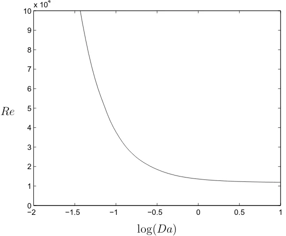
Figure 1: Visual representation of the Poiseuille flow linear instability thresh-olds with critical Reynthresh-olds number Replotted against log(Da).
For Poiseuille flow, the numerical results correspond to comparable stud-ies on Brinkman flow [39]. Couette flow does not yield instability thresholds utilising linear theory.
5.2
Nonlinear stability
In order to study the nonlinear stability of the laminar flows (4.2) we follow the same arguments as in Section 3 but modifying the notations slightly. More precisely, we introduce the functional
F(U,u)≡ kuk2
2+ Da k∇uk22+ Re
Z
Ωp
U0uwdV
!
kuk2 2
, (5.10)
and set
γ(ax, ay)≡ min u∈Ip
where the space of the kinematically admissible perturbationsIp is the space of the divergence-free vector fields u defined in Ωp such that
u −π ax , y, z
=u
π ax
, y, z
∀(y, z)∈
−π ay , π ay
×[0,1],
u
x,−π
ay, z
=u
x, π ay, z
∀(x, z)∈
−π ax, π ax
×[0,1],
u(x, y,0) =u(x, y,1) =0 ∀(x, y)∈
−π ax , π ax × −π ay , π ay . (5.12) In this way, we may state that if γp(ax, ay) >0 then the laminar flow (4.2) is nonlinearly exponentially stable with respect to all perturbations periodic along x and y direction with periods 2π/ax and 2π/ay as
ku(·, t)k2
2 ≤ ku(·,0)k 2 2exp
−2γp(ax, ay)
DaRe t
∀u∈ Ip. (5.13)
The Euler-Lagrange equations corresponding to the variational problem (5.11) are
∇χ+ (1−σ)u−Da∆u+ 1
2DaReU
0
(wi+uk) =0, divu= 0,
(5.14)
where χ is a Lagrange multiplier associated with the incompressibility con-straint. Then, the numberγp(ax, ay) is the least eigenvalueσof the characteristic-value problem (5.14)and (5.12).
Since the Euler-Lagrange equations (5.14) are linear we may follow the same arguments as those employed for the linear stability analysis. More specifically, we take the third components of curl and curlcurl of (5.14)1, use (5.6)3 and (5.14)2 and look for solutions of the form
(
w(x, y, z) = W(z) exp[i(axx+ayy)],
ζ(x, y, z) = curlu·k= Ψ(z) exp[i(axx+ayy)]
(5.15)
to reduce the eigenvalue problem (5.14) and (5.12) to
Da(D2−a2)2W + (σ−1)(D2−a2)W
+DaRe
2 (2iaxU
0
DW +iayU0Ψ +iaxU00W) = 0,
Da(D2−a2)Ψ + (σ−1)Ψ +DaRe 2 iayU
0W = 0,
W =DW = Ψ = 0 atz = 0,1.
Finally, from (28) we may state the following theorem.
Theorem 2. Assume that
γcr≡ min ax,a,y>0
γp(ax, ay)>0. (5.17)
Then the laminar flow (4.2) is globally exponentially stable.
The sixth-order system (5.16) was solved using the Chebyshev-tau method [38]. We let ax =a
√
γ and ay =a
√
1−γ, such that γ ∈ [0, 1] for the range of ax and ay values which comprise wavenumber a.
−2.50 −2 −1.5 −1 −0.5 0 0.5 1
100 200 300 400 500 600 700 800 900 1000
γ = 0
γ = 1 Re
log(Da)
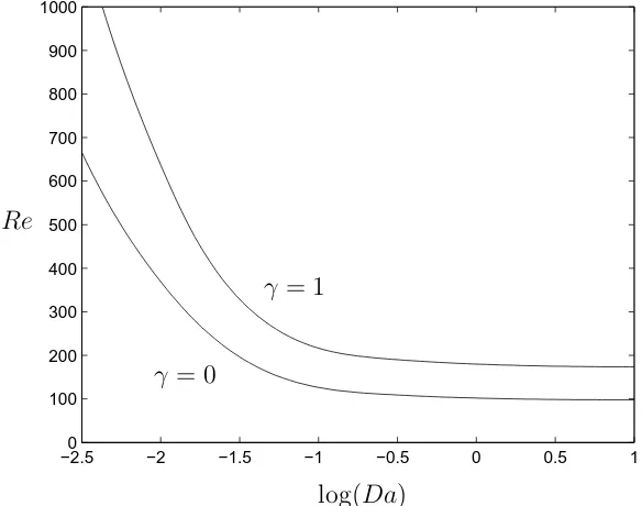
Figure 2: Visual representation of the Poiseuille flow nonlinear stability thresholds with critical Reynolds number Re plotted against log(Da.) The thresholds for γ values between 0 and 1 are contained between theγ = 0 and γ = 1 lines.
[image:13.595.140.432.299.529.2]−2.50 −2 −1.5 −1 −0.5 0 0.5 1 100
200 300 400 500 600 700 800 900 1000
γ = 0
γ = 1 Re
[image:14.595.140.432.128.366.2]log(Da)
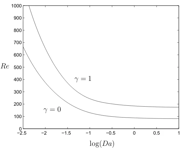
Figure 3: Visual representation of the couette flow nonlinear stability thresh-olds with critical Reynthresh-olds number Replotted against log(Da.) The thresh-olds for γ values between 0 and 1 are contained between theγ = 0 andγ = 1 lines.
Although there is some quantitative differences with Poiseuille flow, the couette flow nonlinear stability thresholds follow a similar formation.
References
[1] H. C. Brinkman, A calculation of the viscous force exerted by a flow-ing fluid on a dense swarm of particles, Applied Scientific Research A1 (1947), 27–34.
[2] H. C. Brinkman, On the permeability of the media consisting of closely packed porous particles, Applied Scientific Research A1 (1947), 81–86.
[3] H. Darcy, La Fontaines Publiques de La Ville de Dijon, Victor Dalmont (1846).
[4] P. Forchheimer,Wasserbewegung durch Boden, Zeits. V. deutsch. Ing45
(1901), 1782–1788.
law and the continuum theory of mixtures, Mathematical Modeling and Methods in Applied Science 3 (1993), 231–248.
[6] S. C. Subramaniam, K. R. Rajagopal, A note on the ow through porous solids at high pressures, Computers and Mathematics with Applications
53 (2007), 260–275.
[7] K. Kannan, K. R. Rajagopal, Flow through porous media due to high pressure gradients, Applied Mathematics and Computations199(2008), 748–759.
[8] K. R. Rajagopal, Hierarchy of models for the flow of fluids through porous media, Mathematical Model and Methods in the Applied Sci-ences 17 (2007), 215–252.
[9] C. Truesdell, Sulle basi della termomeccanica, Rendiconti dei Lincei 22
(1957), 33–38.
[10] C. Truesdell, Sulla basi della termomeccanica, Rendiconti dei Lincei 22
(1957), 158–166.
[11] R. M. Bowen, Mechanics of Mixtures, in Continuum Physics, ed. A. C. Eringen, Vol III, Academic Press (1976).
[12] R. J. Atkin, R. E. Craine, Continuum theory of mixtures: basic the-ory and historical developments, Quarterly Journal of Mechanics and Applied Mathematics 29 (1976), 209–234.
[13] I. Samohyl,Thermodynamics of Irreversible processes in Fluid Mixtures, Teubner (1987).
[14] K. R. Rajagopal, L. Tao, Mechanics of Mixtures, World Scientific Press, Singapore (1995).
[15] G. Johnson, M. Massoudi, K. R. Rajagopal, A review of interaction mechanisms in fluid-solid flows, DOE Report, DOE/PETC/TR-90/9, Pittsburgh (1990).
[16] O. Reynolds, On the dynamical theory of incompressible viscous fluids and the determination of the criterion, Phil. Trans. Roy. Soc. London A
186 (1895), 123–164.
[18] J. L. Synge, Hydrodynamical stability, Semi-centennial publications of the Amer. Math. Soc. 2(1938), 227–269.
[19] J. Kampe de Feriet,Sur la decroissance de l’´energie cin´etique d’un fluide visqueux incompressible occupant un domaine born´e ayant pour fronti`ere des parois solides fixes, Ann. Soc. Sci. Bruxelles 63 (1949), 35–46.
[20] R. Berker, In´egalit´e v´erifi´ee par l’´energie cin´etique d’un fluide visqueux incompressible occupant un domaine spatial born´e, Bull. Tech. Univ. Is-tanbul 2(1949), 41–50.
[21] T. Y. Thomas,On the stability of viscous fluids, Univ. Calif. Publ. Math. New Series 2 (1944), 13–43.
[22] E. Hopf, On non-linear partial differential equations, Lecture series of the symposium on partial differential equations, University of California (1955), 7–11.
[23] J. Serrin, On the stability of viscous fluid motions, Archive for Rational Mechanics and Analysis 3 (1959), 1–13.
[24] Y. Qin, P. N. Kaloni, Convective instabilities in anisotropic porous me-dia, Stud. Appl. Math. 91 (1999), 189–204.
[25] Y. Qin, P. N. Kaloni, Spatial decay estimates for plane flows in the Brinkman-Forchheimer model, Q. Appl. Math. 56 (1998), 71–87.
[26] Y. Qin, J. Guo, P. N. Kaloni, Double diffusive penetrative convection in a porous media, Intl. Engng. Sci. 33 (1995), 303–312.
[27] J. Guo, P. N. Kaloni, Double diffusive convection in porous medium, non-linear stability and the Brinkman effect, Stud. Appl. Math. 94
(1995) 351–358.
[28] F. Franchi, B. Straughan,Structural stability for the Brinkman equation in porous media, Mathematical Methods in the Applied Sciences 19
(1996), 1335–1347.
[29] L. E. Payne, B. Straughan, Stability in initial time geometry for the Brinkman and Darcy equations of flow in porous media, J. Math. Pures Appl. 25 (1996), 225–271.
[31] A. Oberbeck, Uber die Bewegungsercheinungen der Atmosphere, Sitz. Ber. K. Preuss Academy (1888), 383–395.
[32] J. Boussinesq, Theorie Analytique de la Chaleur, Gauthier-Villars (1903).
[33] K. R. Rajagopal, M. Ruzicka, A. R. Srinivasa, On the Oberbeck-Boussinesq equations, Mathematical Models and Methods in the Applied Sciences 6 (1996), 1157–1167.
[34] B. Straughan, Stability and wave motion in porous media, Appl. Math. Sci. Ser. 165, Springer-Verlag (2008).
[35] L. E. Payne, H. F. Weinberger,An optimal Poincar´e inequality for con-vex domains, Archive for Rational Mechanics and Analysis 5 (1960), 286–292.
[36] O. Ladyzhenskaya, The mathematical theory of viscous incompressible flow, Gordon and Breach, New York (1969).
[37] S. Rionero, Metodi variazionali per la stabilit´a asintotica in media in magnetoidrodinamica, Ann. Mate. Pura Appl. 78 (1968), 339–364.
[38] J. J. Dongarra, B. Straughan, D. W. Walker, Chebyshev tau-QZ algo-rithm methods for calculating spectra of hydrodynamic stability problems, Appl. Numer. Math. 22 (1996), 399–434.