A Simple Pattern matching Algorithm for Recovering Empty Nodes and their Antecedents

A simple pattern-matching algorithm for recovering empty nodes

and their antecedents

Mark Johnson

Brown Laboratory for Linguistic Information Processing Brown University

Mark [email protected]

Abstract

This paper describes a simple pattern-matching algorithm for recovering empty nodes and identifying their co-indexed an-tecedents in phrase structure trees that do not contain this information. The pat-terns are minimal connected tree frag-ments containing an empty node and all other nodes co-indexed with it. This pa-per also proposes an evaluation proce-dure for empty node recovery proceproce-dures which is independent of most of the de-tails of phrase structure, which makes it possible to compare the performance of empty node recovery on parser output with the empty node annotations in a gold-standard corpus. Evaluating the algorithm on the output of Charniak’s parser (Char-niak, 2000) and the Penn treebank (Mar-cus et al., 1993) shows that the pattern-matching algorithm does surprisingly well on the most frequently occuring types of empty nodes given its simplicity.

1 Introduction

One of the main motivations for research on pars-ing is that syntactic structure provides important in-formation for semantic interpretation; hence syntac-tic parsing is an important first step in a variety of

∗ _{I would like to thank my colleages in the Brown} Labora-tory for Linguistic Information Processing (BLLIP) as well as Michael Collins for their advice. This research was supported by NSF awards DMS 0074276 and ITR IIS 0085940.

useful tasks. Broad coverage syntactic parsers with good performance have recently become available (Charniak, 2000; Collins, 2000), but these typically produce as output a parse tree that only encodes lo-cal syntactic information, i.e., a tree that does not include any “empty nodes”. (Collins (1997) dis-cusses the recovery of one kind of empty node, viz., WH-traces). This paper describes a simple pattern-matching algorithm for post-processing the output of such parsers to add a wide variety of empty nodes to its parse trees.

Empty nodes encode additional information about non-local dependencies between words and phrases which is important for the interpretation of construc-tions such as WH-quesconstruc-tions, relative clauses, etc.1

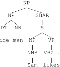
For example, in the noun phrasethe man Sam likes the factthe manis interpreted as the direct object of the verblikesis indicated in Penn treebank notation by empty nodes and coindexation as shown in Fig-ure 1 (see the next section for an explanation of why likesis taggedVBZ trather than the standardVBZ). The broad-coverage statistical parsers just men-tioned produce a simpler tree structure for such a rel-ative clause that contains neither of the empty nodes just indicated. Rather, they produce trees of the kind shown in Figure 2. Unlike the tree depicted in Fig-ure 1, this type of tree does not explicitly represent the relationship betweenlikesandthe man.

This paper presents an algorithm that takes as its input a tree without empty nodes of the kind shown

1_{There are other ways to represent this information that do} not require empty nodes; however, information about non-local dependencies must be represented somehow in order to interpret these constructions.

NP

NP

DT

the NN

man

SBAR

WHNP-1

-NONE-0

S

NP

NNP

Sam

VP

VBZ t

likes NP

-NONE-*T*-1

Figure 1: A tree containing empty nodes.

in Figure 2 and modifies it by inserting empty nodes and coindexation to produce a the tree shown in Fig-ure 1. The algorithm is described in detail in sec-tion 2. The standard Parseval precision and recall measures for evaluating parse accuracy do not mea-sure the accuracy of empty node and antecedent re-covery, but there is a fairly straightforward extension of them that can evaluate empty node and antecedent recovery, as described in section 3. The rest of this section provides a brief introduction to empty nodes, especially as they are used in the Penn Treebank.

Non-local dependencies and displacement phe-nomena, such as Passive and WH-movement, have been a central topic of generative linguistics since its inception half a century ago. However, current linguistic research focuses on explaining the pos-sible non-local dependencies, and has little to say about how likely different kinds of dependencies are. Many current linguistic theories of non-local dependencies are extremely complex, and would be difficult to apply with the kind of broad coverage de-scribed here. Psycholinguists have also investigated certain kinds of non-local dependencies, and their theories of parsing preferences might serve as the basis for specialized algorithms for recovering cer-tain kinds of non-local dependencies, such as WH dependencies. All of these approaches require con-siderably more specialized linguitic knowledge than the pattern-matching algorithm described here. This algorithm is both simple and general, and can serve as a benchmark against which more complex ap-proaches can be evaluated.

NP

NP

DT

the NN

man

SBAR

S

NP

NNP

Sam VP

VBZ t

likes

Figure 2: A typical parse tree produced by broad-coverage statistical parser lacking empty nodes.

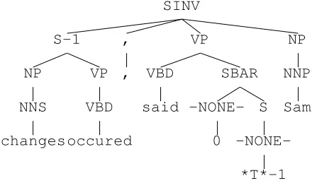
The pattern-matching approach is not tied to any particular linguistic theory, but it does require a tree-bank training corpus from which the algorithm ex-tracts its patterns. We used sections 2–21 of the Penn Treebank as the training corpus; section 24 was used as the development corpus for experimen-tation and tuning, while the test corpus (section 23) was used exactly once (to obtain the results in sec-tion 3). Chapter 4 of the Penn Treebank tagging guidelines (Bies et al., 1995) contains an extensive description of the kinds of empty nodes and the use of co-indexation in the Penn Treebank. Table 1 contains summary statistics on the distribution of empty nodes in the Penn Treebank. The entry with POS SBAR and no label refers to a “compound” type of empty structure labelledSBARconsisting of an empty complementizer and an empty (moved)S

(thusSBARis really a nonterminal label rather than a part of speech); a typical example is shown in Figure 3. As might be expected the distribution is highly skewed, with most of the empty node tokens belonging to just a few types. Because of this, a sys-tem can provide good average performance on all empty nodes if it performs well on the most frequent types of empty nodes, and conversely, a system will perform poorly on average if it does not perform at least moderately well on the most common types of empty nodes, irrespective of how well it performs on more esoteric constructions.

2 A pattern-matching algorithm

Antecedent POS Label Count Description

NP NP * 18,334 NP trace (e.g.,Sam was seen *)

NP * 9,812 NP PRO (e.g.,* to sleep is nice)

WHNP NP *T* 8,620 WH trace (e.g.,the woman who you saw *T*)

*U* 7,478 Empty units (e.g.,$25 *U*)

0 5,635 Empty complementizers (e.g.,Sam said 0 Sasha snores)

S S *T* 4,063 Moved clauses (e.g.,Sam had to go, Sasha explained *T*)

WHADVP ADVP *T* 2,492 WH-trace (e.g.,Sam explained how to leave *T*)

SBAR 2,033 Empty clauses (e.g.,Sam had to go, Sasha explained (SBAR))

WHNP 0 1,759 Empty relative pronouns (e.g.,the woman 0 we saw)

WHADVP 0 575 Empty relative pronouns (e.g.,no reason 0 to leave)

Table 1: The distribution of the 10 most frequent types of empty nodes and their antecedents in sections 2– 21 of the Penn Treebank (there are approximately 64,000 empty nodes in total). The “label” column gives the terminal label of the empty node, the “POS” column gives its preterminal label and the “Antecedent” column gives the label of its antecedent. The entry with anSBARPOS and empty label corresponds to an empty compoundSBARsubtree, as explained in the text and Figure 3.

SINV

S-1

NP

NNS

changes VP

VBD

occured ,

,

VP

VBD

said

SBAR

-NONE-0 S

-NONE-*T*-1 NP

NNP

Sam

Figure 3: A parse tree containing an empty com-poundSBARsubtree.

be regarded as an instance of the Memory-Based Learning approach, where both the pattern extrac-tion and pattern matching involve recursively visit-ing all of the subtrees of the tree concerned. It can also be regarded as a kind of tree transformation, so the overall system architecture (including the parser) is an instance of the “transform-detransform” ap-proach advocated by Johnson (1998). The algorithm has two phases. The first phase of the algorithm extracts the patterns from the trees in the training corpus. The second phase of the algorithm uses these extracted patterns to insert empty nodes and index their antecedents in trees that do not contain empty nodes. Before the trees are used in the train-ing and insertion phases they are passed through a

common preproccessing step, which relabels preter-minal nodes dominating auxiliary verbs and transi-tive verbs.

2.1 Auxiliary and transitivity annotation

The preprocessing step relabels auxiliary verbs and transitive verbs in all trees seen by the algorithm. This relabelling is deterministic and depends only on the terminal (i.e., the word) and its preterminal label. Auxiliary verbs such asisandbeingare relabelled as either aAUXor AUXGrespectively. The relabelling of auxiliary verbs was performed primarily because Charniak’s parser (which produced one of the test corpora) produces trees with such labels; experi-ments (on the development section) show that aux-iliary relabelling has little effect on the algorithm’s performance.

The transitive verb relabelling suffixes the preter-minal labels of transitive verbs with “ t”. For ex-ample, in Figure 1 the verblikesis relabelledVBZ t

in this step. A verb is deemed transitive if its stem is followed by anNPwithout any grammatical func-tion annotafunc-tion at least 50% of the time in the train-ing corpus; all such verbs are relabelled whether or not any particular instance is followed by anNP.

SBAR

WHNP-1

-NONE-0

S

NP VP

VBZ t NP

-NONE-*T*-1

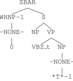
Figure 4: A pattern extracted from the tree displayed in Figure 1.

accuracy of transitivity labelling was not systemati-cally evaluated here.

2.2 Patterns and matchings

Informally, patterns are minimal connected tree fragments containing an empty node and all nodes co-indexed with it. The intuition is that the path from the empty node to its antecedents specifies im-portant aspects of the context in which the empty node can appear.

There are many different possible ways of realiz-ing this intuition, but all of the ones tried gave ap-proximately similar results so we present the sim-plest one here. The results given below were gener-ated where the pattern for an empty node is the min-imal tree fragment (i.e., connected set of local trees) required to connect the empty node with all of the nodes coindexed with it. Any indices occuring on nodes in the pattern are systematically renumbered beginning with 1. If an empty node does not bear an index, its pattern is just the local tree containing it. Figure 4 displays the single pattern that would be extracted corresponding to the two empty nodes in the tree depicted in Figure 1.

For this kind of pattern we define pattern match-inginformally as follows. Ifp is a pattern and tis

a tree, thenpmatchestifftis an extension ofp

ig-noring empty nodes inp. For example, the pattern

displayed in Figure 4 matches the subtree rooted un-derSBARdepicted in Figure 2.

If a pattern pmatches a treet, then it is possible

tosubstitute pfor the fragment oftthat it matches. For example, the result of substituting the pattern

shown in Figure 4 for the subtree rooted underSBAR

depicted in Figure 2 is the tree shown in Figure 1. Note that the substitution process must “standardize apart” or renumber indices appropriately in order to avoid accidentally labelling empty nodes inserted by two independent patterns with the same index.

Pattern matching and substitution can be defined more rigorously using tree automata (G´ecseg and Steinby, 1984), but for reasons of space these def-initions are not given here.

In fact, the actual implementation of pattern matching and substitution used here is considerably more complex than just described. It goes to some lengths to handle complex cases such as adjunction and where two or more empty nodes’ paths cross (in these cases the pattern extracted consists of the union of the local trees that constitute the patterns for each of the empty nodes). However, given the low frequency of these constructions, there is prob-ably only one case where this extra complexity is justified: viz., the empty compound SBARsubtree shown in Figure 3.

2.3 Empty node insertion

Suppose we have a rank-ordered list of patterns (the next subsection describes how to obtain such a list). The procedure that uses these to insert empty nodes into a tree t not containing empty nodes is as

fol-lows. We perform a pre-order traversal of the sub-trees of t (i.e., visit parents before their children),

and at each subtree we find the set of patterns that match the subtree. If this set is non-empty we sub-stitute the highest ranked pattern in the set into the subtree, inserting an empty node and (if required) co-indexing it with its antecedents.

Note that the use of a pre-order traversal effec-tively biases the procedure toward “deeper”, more embedded patterns. Since empty nodes are typi-cally located in the most embedded local trees of patterns (i.e., movement is usually “upward” in a tree), if two different patterns (corresponding to dif-ferent non-local dependencies) could potentially in-sert empty nodes into the same tree fragment int,

shal-lower patterns contain less structure they are likely to match a greater variety of trees than the deeper patterns, they still have ample opportunity to apply.

Finally, the pattern matching process can be speeded considerably by indexing patterns appropri-ately, since the number of patterns involved is quite large (approximately 11,000). For patterns of the kind described here, patterns can be indexed on their topmost local tree (i.e., the pattern’s root node label and the sequence of node labels of its children).

2.4 Pattern extraction

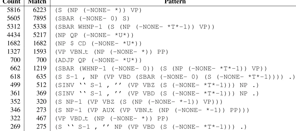
After relabelling preterminals as described above, patterns are extracted during a traversal of each of the trees in the training corpus. Table 2 lists the most frequent patterns extracted from the Penn Tree-bank training corpus. The algorithm also records how often each pattern was seen; this is shown in the “count” column of Table 2.

The next step of the algorithm determines approx-imately how many times each pattern can match some subtree of a version of the training corpus from which all empty nodes have been removed (regard-less of whether or not the corresponding substitu-tions would insert empty nodes correctly). This in-formation is shown under the “match” column in Ta-ble 2, and is used to filter patterns which would most often be incorrect to apply even though they match. Ifcis the count value for a pattern andmis its match value, then the algorithm discards that pattern when the lower bound of a 67% confidence interval for its success probability (givencsuccesses out ofm

tri-als) is less than 1_/2. This is a standard technique for “discounting” success probabilities from small sample size data (Witten and Frank, 2000). (As ex-plained immediately below, the estimates ofcandm

given in Table 2 are inaccurate, so whenever the es-timate ofmis less thancwe replacembycin this

calculation). This pruning removes approximately 2,000 patterns, leaving 9,000 patterns.

The match value is obtained by making a second pre-order traversal through a version of the train-ing data from which empty nodes are removed. It turns out that subtle differences in how the match value is obtained make a large difference to the algo-rithm’s performance. Initially we defined the match value of a pattern to be the number of subtrees that match that pattern in the training corpus. But as

ex-plained above, the earlier substitution of a deeper pattern may prevent smaller patterns from applying, so this simple definition of match value undoubt-edly over-estimates the number of times shallow pat-terns might apply. To avoid this over-estimation, af-ter we have matched all pataf-terns against a node of a training corpus tree we determine the correct pat-tern (if any) to apply in order to recover the empty nodes that were originally present, and reinsert the relevant empty nodes. This blocks the matching of shallower patterns, reducing their match values and hence raising their success probability. (Undoubt-edly the “count” values are also over-estimated in the same way; however, experiments showed that es-timating count values in a similar manner to the way in which match values are estimated reduces the al-gorithm’s performance).

Finally, we rank all of the remaining patterns. We experimented with several different ranking crite-ria, including pattern depth, success probability (i.e.,

c/m) and discounted success probability. Perhaps

surprisingly, all produced similiar results on the de-velopment corpus. We used pattern depth as the ranking criterion to produce the results reported be-low because it ensures that “deep” patterns receive a chance to apply. For example, this ensures that the pattern inserting an emptyNP *andWHNPcan apply before the pattern inserting an empty comple-mentizer0.

3 Empty node recovery evaluation

The previous section described an algorithm for restoring empty nodes and co-indexing their an-tecedents. This section describes two evaluation procedures for such algorithms. The first, which measures the accuracy of empty node recovery but not co-indexation, is just the standard Parseval eval-uation applied to empty nodes only, viz., precision and recall and scores derived from these. In this evaluation, each node is represented by a triple con-sisting of its category and its left and right string po-sitions. (Note that because empty nodes dominate the empty string, their left and right string positions of empty nodes are always identical).

Let G be the set of such empty node

Count Match Pattern

5816 6223 (S (NP (-NONE- *)) VP)

5605 7895 (SBAR (-NONE- 0) S)

5312 5338 (SBAR WHNP-1 (S (NP (-NONE- *T*-1)) VP))

4434 5217 (NP QP (-NONE- *U*))

1682 1682 (NP $ CD (-NONE- *U*))

1327 1593 (VP VBN t (NP (-NONE- *)) PP)

700 700 (ADJP QP (-NONE- *U*))

662 1219 (SBAR (WHNP-1 (-NONE- 0)) (S (NP (-NONE- *T*-1)) VP))

618 635 (S S-1 , NP (VP VBD (SBAR (-NONE- 0) (S (-NONE- *T*-1)))) .)

499 512 (SINV ‘‘ S-1 , ’’ (VP VBZ (S (-NONE- *T*-1))) NP .)

361 369 (SINV ‘‘ S-1 , ’’ (VP VBD (S (-NONE- *T*-1))) NP .)

352 320 (S NP-1 (VP VBZ (S (NP (-NONE- *-1)) VP)))

346 273 (S NP-1 (VP AUX (VP VBN t (NP (-NONE- *-1)) PP)))

322 467 (VP VBD t (NP (-NONE- *)) PP)

269 275 (S ‘‘ S-1 , ’’ NP (VP VBD (S (-NONE- *T*-1))) .)

Table 2: The most common empty node patterns found in the Penn Treebank training corpus. The Count column is the number of times the pattern was found, and the Match column is an estimate of the number of times that this pattern matches some subtree in the training corpus during empty node recovery, as explained in the text.

derived from the corpus to be evaluated. Then as is standard, the precisionP, recallRand f-scoref are

calculated as follows:

P = |G∩T|

|T|

R = |G∩T|

|G|

f = 2P R

P +R

Table 3 provides these measures for two different test corpora: (i) a version of section 23 of the Penn Treebank from which empty nodes, indices and unary branching chains consisting of nodes of the same category were removed, and (ii) the trees produced by Charniak’s parser on the strings of sec-tion 23 (Charniak, 2000).

To evaluate co-indexation of empty nodes and their antecedents, we augment the representation of empty nodes as follows. The augmented represen-tation for empty nodes consists of the triple of cat-egory plus string positions as above, together with the set of triples of all of the non-empty nodes the empty node is co-indexed with. (Usually this set of antecedents is either empty or contains a single node). Precision, recall and f-score are defined for

these augmented representations as before.

Note that this is a particularly stringent evalua-tion measure for a system including a parser, since it is necessary for the parser to produce a non-empty node of the correct category in the correct location to serve as an antecedent for the empty node. Table 4 provides these measures for the same two corpora described earlier.

Empty node Section 23 Parser output

POS Label P R f P R f

(Overall) 0.93 0.83 0.88 0.85 0.74 0.79

NP * 0.95 0.87 0.91 0.86 0.79 0.82

NP *T* 0.93 0.88 0.91 0.85 0.77 0.81

0 0.94 0.99 0.96 0.86 0.89 0.88

*U* 0.92 0.98 0.95 0.87 0.96 0.92

S *T* 0.98 0.83 0.90 0.97 0.81 0.88

ADVP *T* 0.91 0.52 0.66 0.84 0.42 0.56

SBAR 0.90 0.63 0.74 0.88 0.58 0.70

WHNP 0 0.75 0.79 0.77 0.48 0.46 0.47

Table 3: Evaluation of the empty node restoration procedure ignoring antecedents. Individual results are reported for all types of empty node that occured more than 100 times in the “gold standard” corpus (sec-tion 23 of the Penn Treebank); these are ordered by frequency of occurence in the gold standard. Sec(sec-tion 23 is a test corpus consisting of a version of section 23 from which all empty nodes and indices were removed. The parser output was produced by Charniak’s parser (Charniak, 2000).

Empty node Section 23 Parser output

Antecedant POS Label P R f P R f

(Overall) 0.80 0.70 0.75 0.73 0.63 0.68

NP NP * 0.86 0.50 0.63 0.81 0.48 0.60

WHNP NP *T* 0.93 0.88 0.90 0.85 0.77 0.80

NP * 0.45 0.77 0.57 0.40 0.67 0.50

0 0.94 0.99 0.96 0.86 0.89 0.88

*U* 0.92 0.98 0.95 0.87 0.96 0.92

S S *T* 0.98 0.83 0.90 0.96 0.79 0.87

WHADVP ADVP *T* 0.91 0.52 0.66 0.82 0.42 0.56

SBAR 0.90 0.63 0.74 0.88 0.58 0.70

WHNP 0 0.75 0.79 0.77 0.48 0.46 0.47

4 Conclusion

This paper described a simple pattern-matching al-gorithm for restoring empty nodes in parse trees that do not contain them, and appropriately index-ing these nodes with their antecedents. The pattern-matching algorithm combines both simplicity and reasonable performance over the frequently occur-ing types of empty nodes.

Performance drops considerably when using trees produced by the parser, even though this parser’s precision and recall is around 0.9. Presumably this is because the pattern matching technique requires that the parser correctly identify large tree fragments that encode long-range dependencies not captured by the parser. If the parser makes a single parsing error anywhere in the tree fragment matched by a pattern, the pattern will no longer match. This is not unlikely since the statistical model used by the parser does not model these larger tree fragments. It suggests that one might improve performance by integrating parsing, empty node recovery and an-tecedent finding in a single system, in which case the current algorithm might serve as a useful baseline. Alternatively, one might try to design a “sloppy” pat-tern matching algorithm which in effect recognizes and corrects common parser errors in these construc-tions.

Also, it is undoubtedly possible to build pro-grams that can do better than this algorithm on special cases. For example, we constructed a Boosting classifier which does recover *U* and empty complementizers 0 more accurately than the pattern-matcher described here (although the pattern-matching algorithm does quite well on these constructions), but this classifier’s performance av-eraged over all empty node types was approximately the same as the pattern-matching algorithm.

As a comparison of tables 3 and 4 shows, the pattern-matching algorithm’s biggest weakness is its inability to correctly distinguish co-indexed NP *

(i.e., NP PRO) from free (i.e., unindexed) NP *. This seems to be a hard problem, and lexical infor-mation (especially the class of the governing verb) seems relevant. We experimented with specialized classifiers for determining if anNP *is co-indexed, but they did not perform much better than the algo-rithm presented here. (Also, while we did not

sys-tematically investigate this, there seems to be a num-ber of errors in the annotation of free vs. co-indexed

NP *in the treebank).

There are modications and variations on this al-gorithm that are worth exploring in future work. We experimented with lexicalizing patterns, but the simple method we tried did not improve re-sults. Inspired by results suggesting that the pattern-matching algorithm suffers from over-learning (e.g., testing on the training corpus), we experimented with more abstract “skeletal” patterns, which im-proved performance on some types of empty nodes but hurt performance on others, leaving overall per-formance approximately unchanged. Possibly there is a way to use both skeletal and the original kind of patterns in a single system.

References

Ann Bies, Mark Ferguson, Karen Katz, and Robert Mac-Intyre, 1995. Bracketting Guideliness for Treebank II style Penn Treebank Project. Linguistic Data Consor-tium.

Eugene Charniak. 2000. A maximum-entropy-inspired

parser. In The Proceedings of the North American

Chapter of the Association for Computational Linguis-tics, pages 132–139.

Michael Collins. 1997. Three generative, lexicalised models for statistical parsing. InThe Proceedings of the 35th Annual Meeting of the Association for Com-putational Linguistics, San Francisco. Morgan Kauf-mann.

Michael Collins. 2000. Discriminative reranking for

nat-ural language parsing. In Machine Learning:

Pro-ceedings of the Seventeenth International Conference (ICML 2000), pages 175–182, Stanford, California.

Ferenc G´ecseg and Magnus Steinby. 1984. Tree

Au-tomata. Akad´emiai Kiad´o, Budapest.

Mark Johnson. 1998. PCFG models of

linguis-tic tree representations. Computational Linguistics, 24(4):613–632.

Michell P. Marcus, Beatrice Santorini, and Mary Ann Marcinkiewicz. 1993. Building a large annotated

cor-pus of English: The Penn Treebank. Computational

Linguistics, 19(2):313–330.

Ian H. Witten and Eibe Frank. 2000.Data mining: